Investigating the Impact of Spatial Distribution of Sustainable Drainage System (SuDS) Components on Their Flood Mitigation Performance in Communities with High Groundwater Levels

Abstract

This paper investigated the impact of the spatial distribution of SuDS components on their flood reduction performance and the underlying mechanisms in a community with high groundwater levels. The effects of SuDS components’ connectivity, decentralized level, and installation position along the flow direction on the reduction of total discharge volume (TDV), average discharge flow rate (ADFR), maximum discharge flow rate (MDFR), inundated area (IA), average inundated depth (AID), and maximum inundated depth (MID) were studied by coupling of the storm water management model (SWMM) and high-performance integrated hydrodynamic modelling system (HiPIMS). The results demonstrate that the connectivity has a positive linear correlation with the reduction of TDV (R² > 0.991), ADFR (R² > 0.992), and MDFR (R² > 0.958), while the decentralized level of rain gardens and green roofs present positive one-phase exponential correlation with the reduction of TDV (R² > 0.935), ADFR (R² > 0.934) and MDFR (R² > 0.967). A better-integrated mitigation of TDV and ADFR could be achieved by installing SuDS upstream along the flow direction. The connectivity from green roofs to rain gardens has a positive effect on the reduction of AID and MID but leads to the increase of IA. The findings of this study may contribute to the development of general spatial distribution guidelines and strategies to optimize the overall performance of SuDS components, especially at a community scale.

1. Introduction

Flooding is one of the most common hazards in both the natural environment and urban areas [1,2]. The frequency and severity of floods have increased significantly, leading to growing concerns about the participation of stakeholders from communities [3], the effectiveness of traditional urban drainage infrastructure [4], challenges from the complexity of sustainable technologies [5], and climate change [6]. The recorded floods since 2000 in the UK have affected 433,933 people and caused damage of over 21 million dollars, according to the data from EM-DAT [7]. As greater pressure is put on traditional urban water management systems due to the urbanization process and the increase in human activities, the water quality of rivers and coastal aquifers tends to deteriorate [8,9]. Rapid urbanization has brought great landscape changes and land-use adjustment in urban areas [10,11] and interacts with climate change to increase the risk of urban flooding [12,13]. These changes include replacement of permeable lands with impervious areas and removal of vegetation, leading to an increase of peak flow and rainwater runoff [14,15]. On the other hand, climate changes are widely believed to increase the risk of urban flooding by aggrandizing the frequency and duration of heavy rainfall events [16] and increasing the difficulty of flood forecasting [17,18,19], causing large economic losses due to house collapse and drainage system maintenance [16,20]. Unfortunately, it has become increasingly difficult for the traditional urban drainage system to adapt to these changes. Therefore, more countries have moved towards risk-based sustainable management to improve the flood resilience of urban areas [21,22,23]. Among the terminology used to describe the sustainable management strategies, Sustainable Drainage System (SuDS) is used in this paper.

The Sustainable Drainage System (SuDS) was designed to minimize the risk of urban flooding and maximize the opportunities and benefits in terms of water quantity, water quality, amenity and biodiversity [24,25]. First proposed by the UK government, SuDS has been proven to be effective in storm water management and flood risk mitigation for specific precipitation characteristics [26,27,28]. Zahmatkesh et al. studied the impact of SuDS implementation on runoff reduction in New York City’s urban catchment for future climate change prediction and indicated that SuDS has a potential mitigation effect on the runoff and peak flow [29]. Compared to traditional approaches, SuDS has better performance in reducing the storm flow, peak discharge and most water quality indicators [30]. The implementation of SuDS can also mitigate runoff pollutants and heat islands due to urbanization, having a positive impact on achieving water balance and water reuse [29,31,32].

The spatial distribution of SuDS components within a specific catchment strongly influences their effectiveness in flood reduction. Recent studies have explored the effect of spatial distribution patterns on surface runoff, thus providing more general spatial distribution optimization recommendations for SuDS practices at urban or larger catchment scales [33,34]. Kim and Park believe that the use of landscape indicators can help the design of SuDS spatial layouts, especially for urban green infrastructure such as rain gardens and bio-retentions [35]. They point out that increasing the size, fragmentation and connectivity of these components can reduce peak runoff on a macro scale [35]. Mejia and Moglen clarified that when determining the hydrological response of urban watersheds, it is necessary to consider both the precipitation characteristics and the spatial variability of impermeability [36]. Similarly, Liang, You and Lee studied the SuDS layout through genetic algorithm (GA) and hydrological analysis and suggested that SuDS facilities with storage layers should be concentrated in the middle reaches of drainage trunk lines to efficiently reduce surface runoff and delay the time to peak flow [37].

Site constraints are important factors in optimizing spatial distribution, as they may limit the scope of selecting SuDS components and their flood mitigation efficiency. Common site constraints include land use type, pollution loading, soil type and depth, groundwater level, topography, available space, drainage system and impervious area [38]. Changes in land use types often lead to alterations in available space and impervious areas, which affect the implementation of SuDS and the hydrological response, especially in urban areas with complex land use types [39]. The research of Zeng, Guo and Dong indicates that the synergy with urban drainage system can effectively improve the flood reduction performance of SuDS [40]. Differences in topography and soil conditions will directly lead to changes in surface runoff and infiltration characteristics, which therefore are other important factors [41]. Shallow water tables and moisture-saturated soils also often limit the implementation of SuDS due to the risk of facility failure and groundwater contamination, especially in coastal areas [42,43]. In this case, SuDS without storage layers may be a more suitable option, because it normally requires smaller installation depth under the ground. However, there are few studies focusing on the spatial distribution of SuDS suitable for areas with high groundwater levels.

Communities are the basic units for urban SuDS planning, and SuDS research at the community scale has gradually received more attention [44]. Besides the government, participation and support from different groups and communities are essential to realize the application of SuDS [45]. Therefore, Latifi et al. proposed a leader–follower game model to balance the conflicting utility that may exist between various participants [46]. Other studies have suggested optimizing the spatial distribution by establishing a multi-standard evaluation framework based on residents’ willingness [47], site constraints [48], urban development planning [49] and cost-benefit analysis [50]. However, the custom weights used in the framework may affect the results of spatial optimization, so its reliability cannot be guaranteed [38]. In this case, the use of hydrological models to assess SuDS performance at the community scale is another option [38]. To better evaluate the runoff control of community-scale SuDS, Yin et al. proposed a SWMM-CADDIES integrated model to analyze the rainfall runoff process in the community [51]. Chen et al. used the enhanced L-THIA-LID 2.2 model to study the effectiveness of SuDS in a combined sewer overflow community and found that the combined implementation of SuDS can reduce runoff and pollutant load more effectively than individual application [52].

Although SuDS research at the community scale is gaining popularity, existing studies on the spatial distribution optimization of SuDS at the community scale are limited in their scope. Some studies have examined the spatial distribution of SuDS components at a community scale, but few studies specifically analyzed the spatial distribution of suitable SuDS components in areas with high groundwater levels. Many scholars have conducted research on the spatial distribution of SuDS at the urban or watershed scales [48,53,54]. However, limited by the diversity of community types and inadequate spatial resolution, these studies cannot be directly applied to the community scale [53]. Kim and Park reported the contracting effects of green infrastructure’s connectivity on reducing surface runoff at different scales [35], highlighting the importance of community-scale study for SuDS distribution. The lack of such studies hinders the effective design of SuDS spatial distribution in practice. Only nine urban typologies are provided in the SuDS manual as design examples to support the specific design of spatial distribution of SuDS components at the community scale [25]. These typologies cannot cover all the complex patterns seen in different communities.

To fill these gaps, this study used the SWMM-HiPIMS coupled model to simulate the impact of SuDS on surface runoff and inundation indicators in different spatial distribution scenarios of a community with high groundwater level, aiming to reveal the relationship between the spatial distribution of SuDS components and the flood reduction as well as the underlying mechanisms from a hydrologic perspective. Green roofs and rain gardens were chosen as the typical SuDS components without storage layers, which are suitable for communities with high groundwater levels. The results of the study may help local designers optimize the spatial distribution of SuDS in communities with high groundwater levels.

2. Materials and Methods

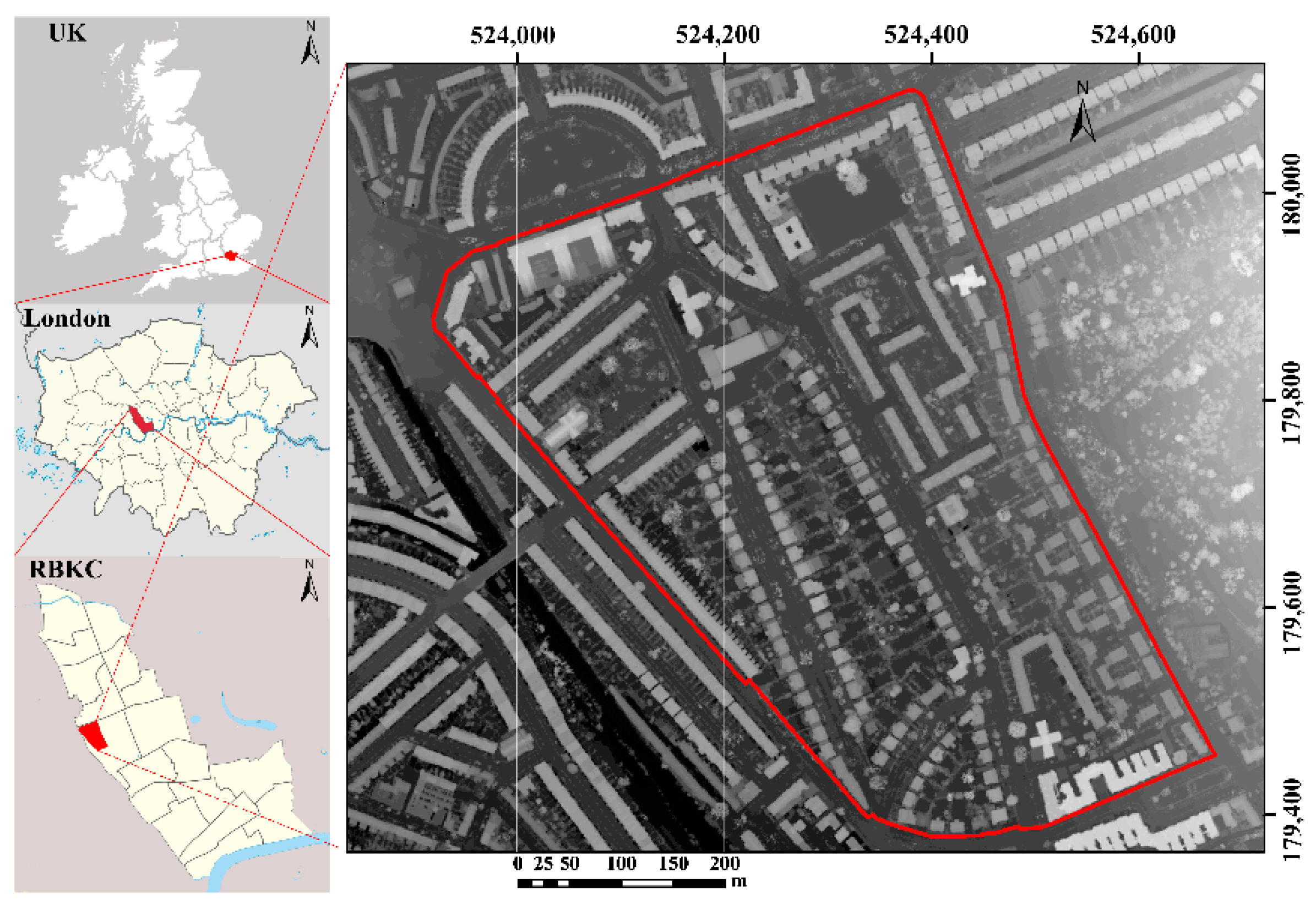
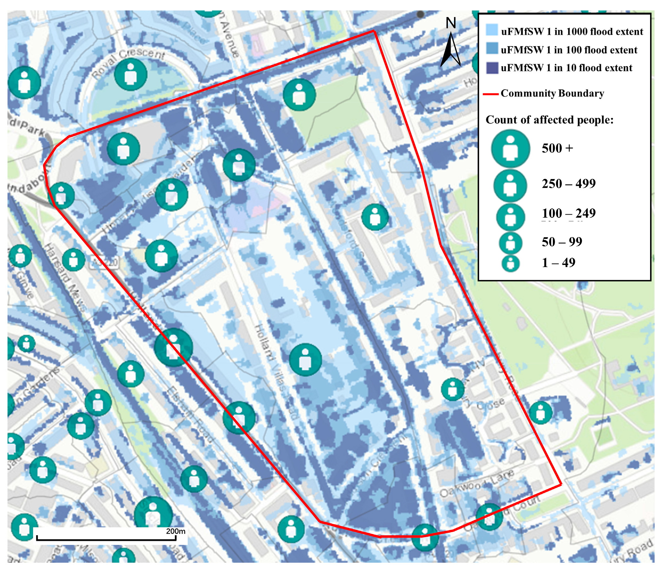
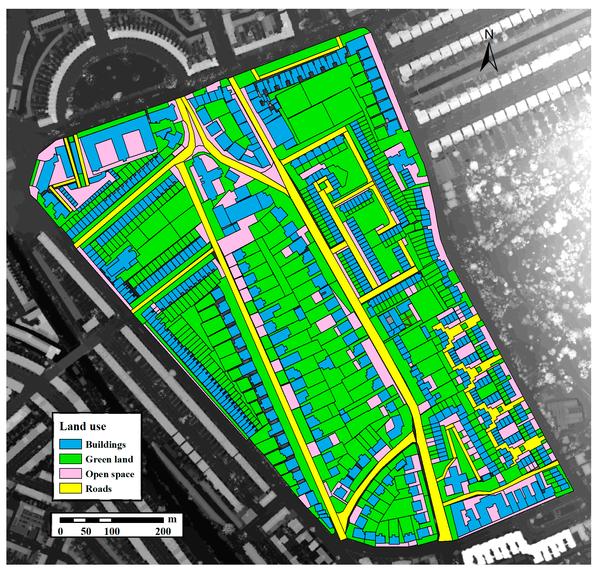
This study investigated the impact of different spatial distribution scenarios of SuDS components on flood reduction at the community scale. In this study, SWMM, one of the most popular rainfall runoff models for urban water resource management, was used to simulate the response of SuDS components to rainfall with different spatial distributions in the first stage. Then, the surface runoff data in the SWMM model running results were fed into the HiPIMS as effective rainfall to simulate the flood inundating process with higher spatial and temporal resolution. The simulation results give the position and area of flood inundation.

2.1. Study Area

The study area (51°30′10″, 0°12′37″) is a community-scale area located in an urban catchment. The urban catchment is part of the drainage system in the Royal Borough of Kensington and Chelsea (RBKC), west London, England (Figure 1). RBKC is the smallest borough in London and one of the most densely populated administrative areas in Britain, with more than 150,000 people living on 1213 hectares. It was chosen mainly because of its relatively high flood risk, according to the 2019 flood risk map for surface water in England (Figure 2) on the Environment Agency website. As shown in Figure 3, the study area has a total size of 28.9 hectares and includes the following four land-use types: buildings, green land, roads and open space.

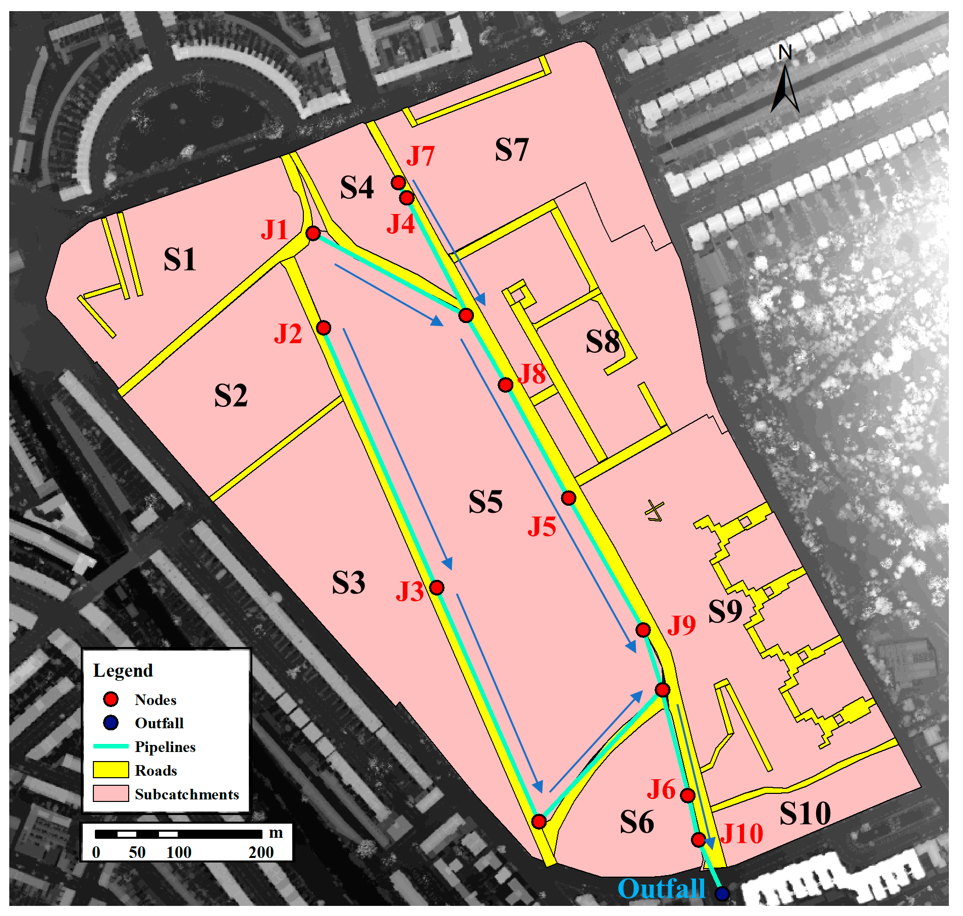
2.2. SWMM Simulation

First developed by the Environmental Protection Agency of the United States (US EPA) in 1971, the Storm Water Management Model (SWMM) is a dynamic rainfall–runoff simulation model used for single-event or long-term simulation of runoff quantity and quality from primarily urban areas [57]. The SuDS components have been included in the model package since Version 5.0.22 [37]. The SWMM software used in this study is Version 5.1.013.

The setup of the SWMM model was based on the data from various online databases. Ten subcatchments, numbered from S1 to S10, were defined by the roads in the study area, under the consensus that drainage pipes are normally laid along the roads. The assumed drainage pipelines were set up along the roads to estimate the total runoff volume, which did not affect the surface runoff state. The subcatchments and drainage system set in the SWMM are shown in Figure 4, with blue arrows showing the flow direction in the pipes. The junctions that allow the subcatchments S1 to S10 to drain are numbered from J1 to J10. The aerial image from Google Earth, with a resolution of 1 m, was used to classify land-use types and identify impermeable areas (buildings, roads and open space) and permeable areas (green land). The land use map of the study area is shown in Figure 3.

In this paper, the subcatchment components were defined specifically as ‘mini-catchments’, referring to the land use map. They were set to drain to the corresponding junctions, named J1 to J10 according to the subcatchments they were located in. The rainwater in the drainage system discharged to the same downstream outlet, namely the Outfall. In summary, there were 10 subcatchments, including 1348 mini-catchments, 13 junctions, 13 conduits and 1 outlet, in the study area.

The surface parameters of the mini-catchments were set up based on the Digital Surface Model (DSM) and Digital Terrain Model (DTM) data, with a resolution of 1 m, which were downloaded from the Defra Data Services Platform. Then the DSM and DTM data were processed to set up the area and average slope for the mini-catchments. The other parameters of mini-catchments were set up according to the SWMM User’s Manual Version 5.1. The land use map and the field soil condition were obtained from the Cranfield Soil and Agrifood Institute [58]. Horton’s equation was used to calculate the infiltration of water into the soil. A summary of the SWMM model parameter settings for the subcatchment components are listed in Table S1, while the infiltration parameter settings for Horton’s equation are summarized in Table S2 in the Supplementary Materials.

The pipelines of the drainage system are assumed to be built from concrete. Therefore, Manning’s roughness coefficient was set to 0.015. It was assumed that every conduit is equipped with flap gates to prevent the backflow of rainwater. The other assumed parameters are summarized in Table S3.

The study area consisted of 45.6% green land, 26.8% buildings, 11.3% roads and 16.3% open space. The large areas of green land had the potential to be converted into rain gardens (RGs), while the roofs of the buildings were the ideal location for green roofs (GRs). The rain garden comprised a surface layer and a soil layer, while the green roof comprised a surface layer, a soil layer and a drainage mat. Both SuDS components included no storage layers and thus were suitable for the study area, where the groundwater level is relatively high [58].

The rainfall runoff on the green roof was to infiltrate into the soil layer and drain off the roof through the drainage mat, while the rainwater in the rain garden was to infiltrate through the engineered soil layer quickly and into the natural soil directly [57]. The schematic diagram of the SuDS components in the SWMM model is shown in Figure S1, and Table S4 summarizes the parameter settings of the SuDS components in the SWMM model. The porosity of the soil layer was defined according to Table S5 in the Supplementary Materials [57].

Due to the limited available data, we set up a hypothetical pipeline system based on data from a similar study [37], as shown in Figure 4 and Table S3 in the Supplementary Materials. The results of rainwater discharge through the outlet could be used to reflect the overall situation of the surface runoff in the study area. Considering that the potential irrationality of the assumed pipeline may be amplified by complex calculations, the relatively simple Kinematic Wave method can not only reduce possible error, but also meet the research requirements to some extent. Therefore, the Kinematic Wave method was used to route flows through the conveyance system. A time step length of 5 s was applied to both the simulations of pipe routing and surface runoff.

2.3. Design Storms

According to the Flood Estimation Handbook (FEH) [59], the depth-duration-frequency (DDF) model is recommended to design rainfall events in the UK. The calculated design rainfall data with various return periods and durations in the study area was accessed on the website of FEH Web Services [60]. As non-riverine urban flooding is generally caused by short-term heavy rainfall events, 1 h (36.39 mm of precipitation) and 3 h rainfall events (52.81 mm of precipitation) with a return period of 30 years were selected as the input rainfall of the SWMM model. The two rainfall events were designed with even rainfall intensity.

2.4. Flood Simulation Configuration

The flood simulations were performed by a GPU-based flood model, HiPIMS. Developed by Xia, Liang and Ming (2019), the high-performance integrated hydrodynamic modelling system (HiPIMS) uses state-of-the-art numerical schemes (Godunov-type finite volume) to solve the 2D shallow water-type equations for flood and landslide simulations [61]. It was developed to predict the full-scale process of fluvial flooding from the source (rainfall) to impact (inundation) over a large catchment using a single high-performance hydrodynamic model driven by rainfall inputs [61].

The same DSM data were used to define the topography of the simulation. The landcover data were utilized to define the Manning’s roughness coefficient of the areas with different landcover types (Table S6). The rainfall inputs were obtained by processing the surface runoff data of the SWMM model for the equivalent rainfall intensity.

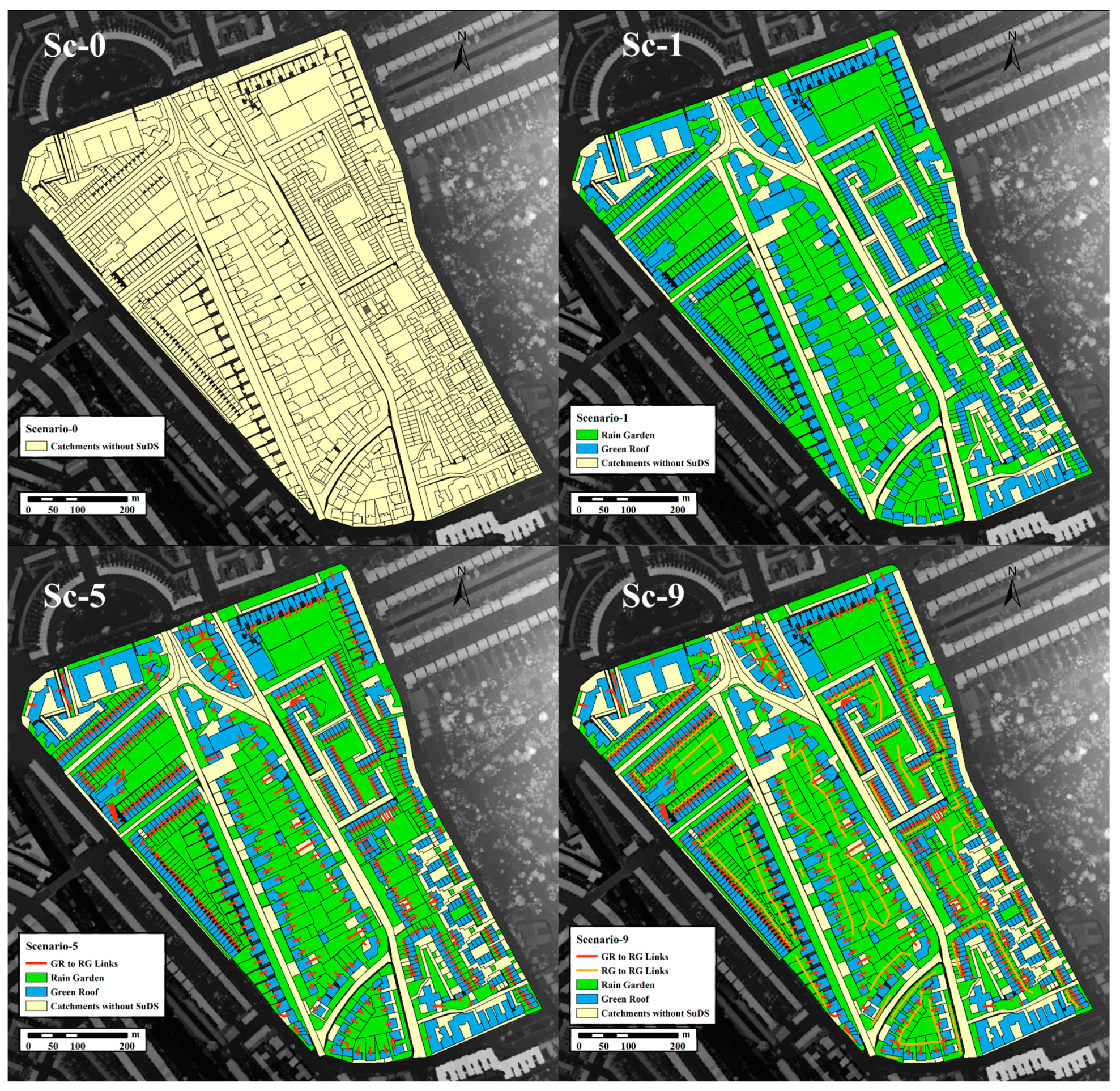
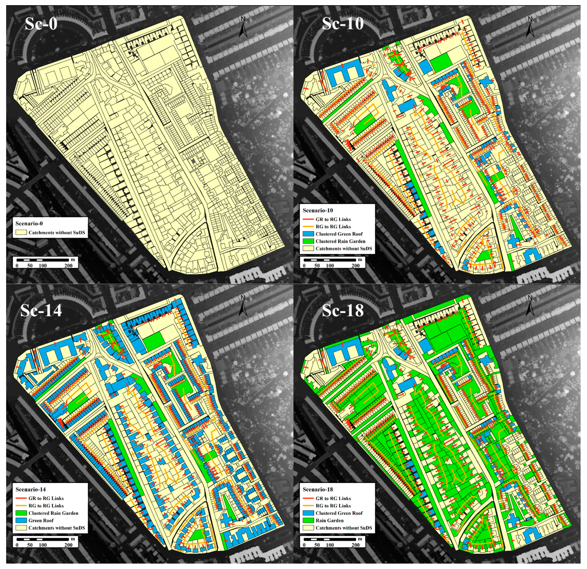
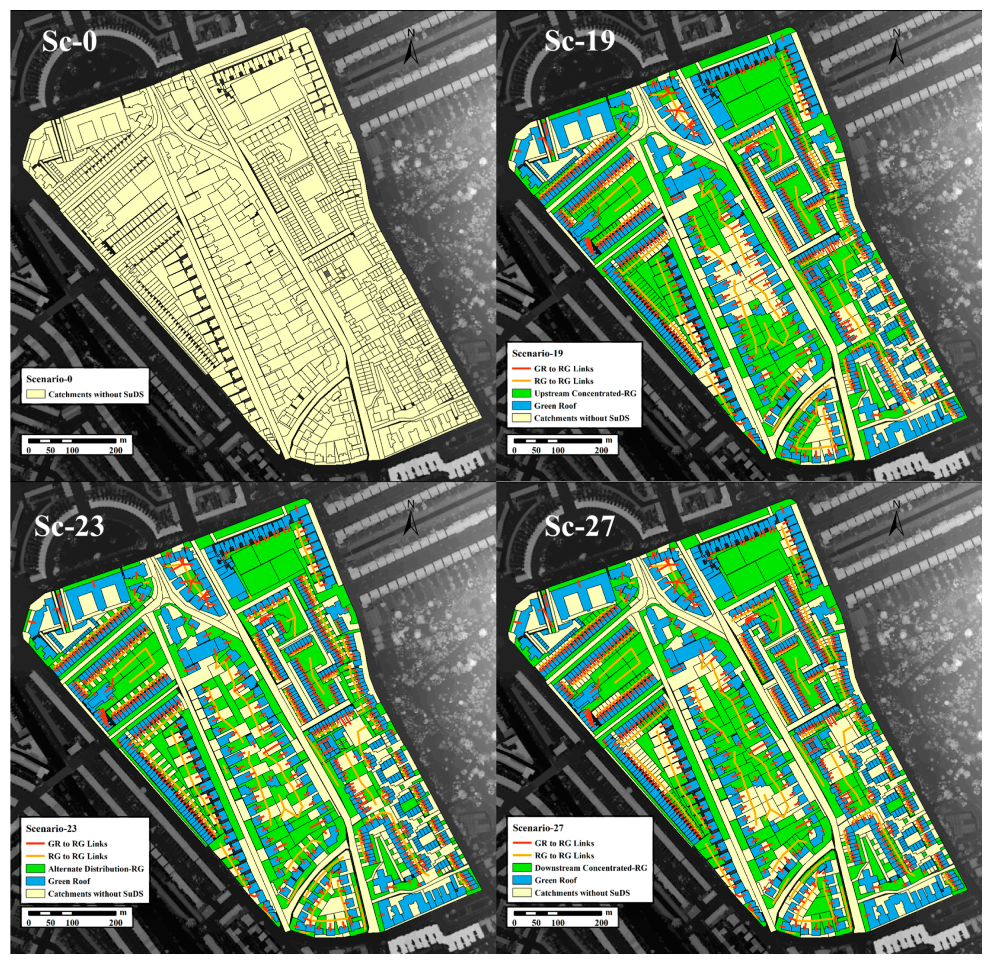
2.5. SuDS Spatial Distribution Scenarios

To study the relationship between the spatial distribution pattern of SuDS components and their overall performance of flood reduction at the community scale, 27 types of spatial distribution scenarios for SuDS and a blank scenario 0 without SuDS were proposed to simulate the flood reduction performance in the SWMM model. Nine sketch maps of the key spatial distribution strategies are provided in Figure 5, Figure 6 and Figure 7. To facilitate the statistics and analysis, the area of each SuDS unit was set to 20 m² due to the area limit (20 m²) of the minimum mini-catchment; all the units can treat the runoff drained from other subcatchments. Each subcatchment could install more than one SuDS unit as long as the total SuDS area did not exceed the total area of the subcatchment. According to the principle of single variable, we set up the combination of multiple SuDS units with an area of 20 m² to avoid the interference of the area change of SuDS units when studying the influence of the decentralized distribution strategy.

The scenarios were designed from three aspects, as shown in Figure 5, Figure 6 and Figure 7. Scenarios 1 to 9 were designed to explore the impact of connectivity between SuDS components on their flood reduction performance. They were followed by scenarios 10 to 18, which were designed to study the impact of the clustering level of SuDS components. Scenarios 19 to 27 were designed to study the SuDS components’ position along the flow direction. The detailed descriptions for sketch maps of 27 scenarios can be found in Figures S2–S28 in the Supplementary Materials. Scenario 0 was also constructed in the SWMM model as a blank control. The distribution strategies of 27 scenarios were provided in

Table 1. Summary of the distribution strategies in scenarios 1 to 27.

Scenarios	Strategy for Rain Gardens	Strategy for Green Roofs
1	527 units decentralized; disconnected	622 units decentralized; disconnected
2	527 units decentralized; disconnected	622 units decentralized; 151 units connected to RG
3	527 units decentralized; disconnected	622 units decentralized; 275 units connected to RG
4	527 units decentralized; disconnected	622 units decentralized; 395 units connected to RG
5	527 units decentralized; disconnected	622 units decentralized; 526 units connected to RG
6	527 units decentralized; 139 units connected	622 units decentralized; 526 units connected to RG
7	527 units decentralized; 235 units connected	622 units decentralized; 526 units connected to RG
8	527 units decentralized; 315 units connected	622 units decentralized; 526 units connected to RG
9	527 units decentralized; 422 units connected	622 units decentralized; 526 units connected to RG
10	527 units clustered; 422 units connected	622 units clustered; 526 units connected to RG
11	527 units clustered; 422 units connected	489 units clustered; 526 units connected to RG
12	527 units clustered; 422 units connected	355 units clustered; 526 units connected to RG
13	527 units clustered; 422 units connected	214 units clustered; 526 units connected to RG
14	527 units clustered; 422 units connected	622 units decentralized; 526 units connected to RG
15	396 units clustered; 422 units connected	622 units clustered; 526 units connected to RG
16	270 units clustered; 422 units connected	622 units clustered; 526 units connected to RG
17	166 units clustered; 422 units connected	622 units clustered; 526 units connected to RG
18	527 units decentralized; 422 units connected	622 units clustered; 526 units connected to RG
19	341 units decentralized; 233 units connected; upstream distributed	622 units clustered; 526 units connected to RG
20	341 units decentralized; 233 units connected; upstream distributed	622 units clustered; 526 units connected to RG
21	341 units decentralized; 233 units connected; upstream distributed	622 units clustered; 526 units connected to RG
22	341 units decentralized; 233 units connected; upstream distributed	622 units clustered; 526 units connected to RG
23	341 units decentralized; 233 units connected; alternately distributed	622 units clustered; 526 units connected to RG
24	341 units decentralized; 233 units connected; downstream distributed	622 units clustered; 526 units connected to RG
25	341 units decentralized; 233 units connected; downstream distributed	622 units clustered; 526 units connected to RG
26	341 units decentralized; 233 units connected; downstream distributed	622 units clustered; 526 units connected to RG
27	341 units decentralized; 233 units connected; downstream distributed	622 units clustered; 526 units connected to RG

. To ensure that only the spatial distribution strategies differ in these scenarios, the number and types of SuDS units applied in the 27 scenarios were controlled as shown in Table S7 in Supplementary Materials.

The connectedness (CONNECT), edge density (ED) and the flow distance (FD) among the outlets and the mini-catchments were chosen as indexes to assess the connectivity, decentralized level and position along the flow direction of the considered scenarios, respectively [35].

The connectedness equals the number of functional joins between mini-catchments of the same type within the catchment, divided by the total number of possible joins between all corresponding mini-catchments, multiplied by 100 [33]:

$$\mathrm{CONNECT}=\frac{{\sum }_{\mathrm{j}-\mathrm{k}}^{\mathrm{n}}{\mathrm{C}}_{\mathrm{ijk}}}{\frac{{\mathrm{n}}_{\mathrm{i}}\left({\mathrm{n}}_{\mathrm{i}}-1\right)}{2}}$$

(1)

where

• C_ijk = number of connections between mini-catchments j and k (0 = disconnected, 1 = connected) of all corresponding mini-catchments in the study area
• n_i = number of mini-catchments in the study area

The edge density equals the total length of the edge divided by the area of all mini-catchments [35]:

$$\mathrm{ED}=\frac{\mathrm{E}}{\mathrm{A}}$$

(2)

where

• E = the sum of edges (m)
• A = total area (m²)

The flow distance refers to the average distance among the outfall nodes of subcatchments S1 to S10 and the mini-catchments with SuDS components in the study area [37]:

$$\mathrm{FD}=\frac{{\sum }_{\mathrm{i}=0}^{\mathrm{n}}{\sum }_{\mathrm{j}=1}^{10}\sqrt{{\left({\mathrm{X}}_{\mathrm{j}}-{\mathrm{x}}_{\mathrm{i}}\right)}^2+{\left({\mathrm{Y}}_{\mathrm{j}}-{\mathrm{y}}_{\mathrm{i}}\right)}^2}}{\mathrm{n}}$$

(3)

where

• X_j = x-coordinate of the outfall nodes in subcatchments S1 to S10 (m)
• Y_j = y-coordinate of the outfall nodes in subcatchments S1 to S10 (m)
• x_i = x-coordinate of the SuDS mini-catchments’ drainage locations (m)
• y_i = y-coordinate of the SuDS mini-catchments’ drainage locations (m)
• n = number of mini-catchments in the study area

The summary of the indexes of the decentralized level, connectivity and the SuDS components’ position along the flow direction in 27 scenarios is shown in Table S8 in the Supplementary Materials.

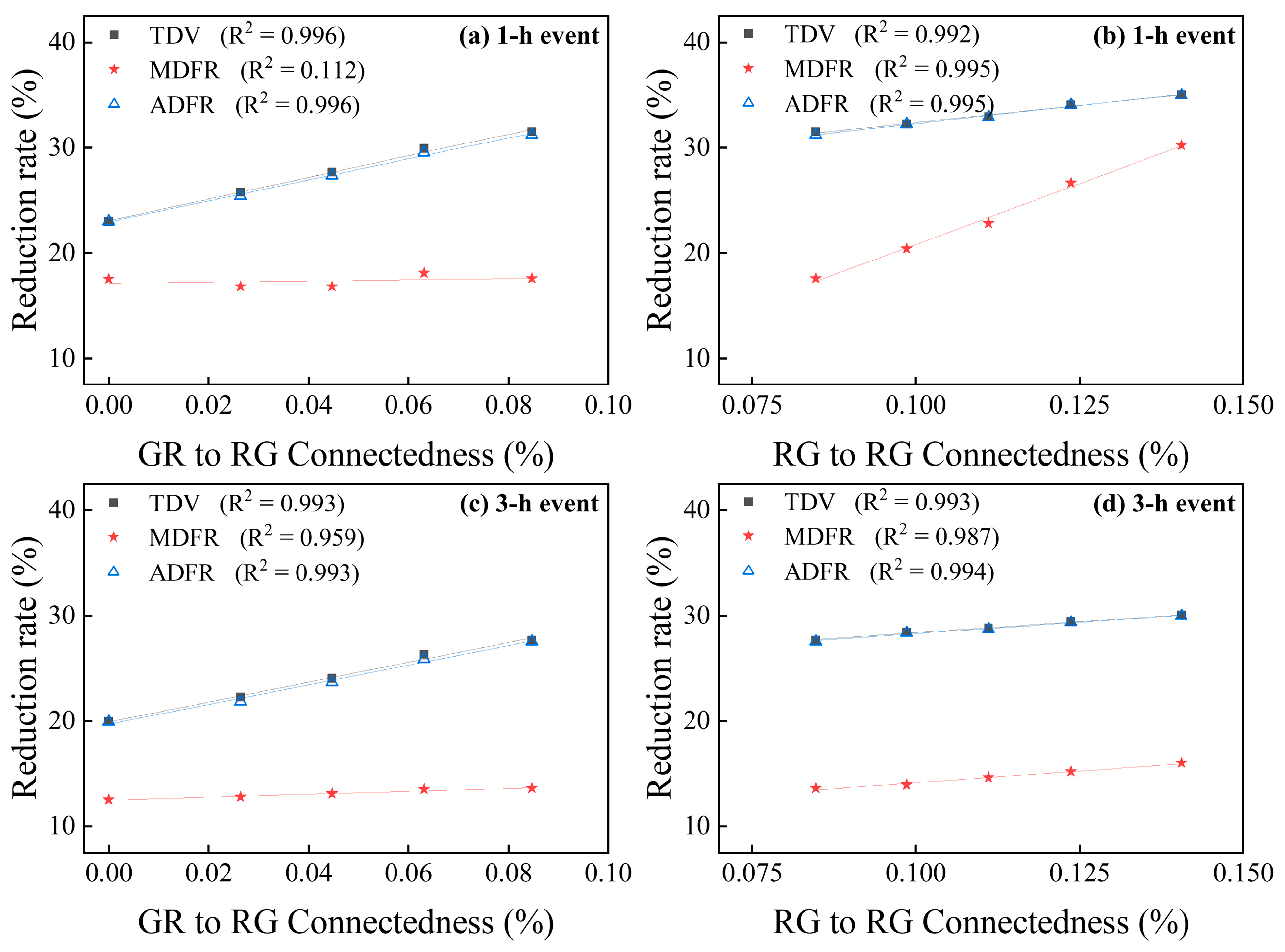
2.6. The Performance Assessment Criteria of Spatial Distribution Scenarios

This SWMM’s summary results report includes the results for each subcatchment, node, and link in the project through a selectable list of tables [57]. Based on this report, the maximum discharge flow rate (MDFR), the average discharge flow rate (ADFR) and the total discharge volume (TDV) of flow drained from the downstream outlet were selected as the main indicators to evaluate the mitigation of surface runoff.

The simulation results at each reporting time step for various variables of subcatchments, nodes, and links are also available to be plotted and statistically analyzed in SWMM [57]. To analyze the changes in surface runoff over the process of the design rainfall, the time series results of the discharge flow rate of downstream outlet were selected as another perspective to assess the flood mitigation performance of the considered scenarios.

The simulation results of HiPIMS include three types: the water depth and velocities at predefined moments during a simulated event, the maximum water depth and velocities throughout the event, and the time series of water depth and velocities, including rainfall over the model domain and inflow and outflow boundary conditions. In this paper, the changes of average inundated depth (AID), maximum inundated depth (MID) and the inundated area (IA) during the rainfall events were selected to study the inundated areas in 27 scenarios.

The simulation results of HiPIMS also reveal the inundated area distribution in these scenarios. Detailed flood maps when the maximum inundated depth occurs in 28 considered scenarios in 1 h and 3 h rainfall events are shown in Figures S29–S84 in the Supplementary Materials.

The correlation coefficient (R²) was chosen to assess the correlation between SuDS components’ spatial characteristics and their flood reduction performance:

$${\mathrm{R}}^2=1-\frac{{\sum }_{\mathrm{i}=1}^{\mathrm{n}}{\left({\mathrm{y}}_{\mathrm{i}} - {\hat{\mathrm{y}}}_{\mathrm{i}}\right)}^2}{{\sum }_{\mathrm{i}=1}^{\mathrm{n}}{\left({\mathrm{y}}_{\mathrm{i}} - {\overline{\mathrm{y}}}_{\mathrm{i}}\right)}^2}$$

(4)

where

• $\sum _{\mathrm{i}=1}^{\mathrm{n}}{\left({\mathrm{y}}_{\mathrm{i}} - {\hat{\mathrm{y}}}_{\mathrm{i}}\right)}^2$ = residual sum of squares
• $\sum _{\mathrm{i}=1}^{\mathrm{n}}{\left({\mathrm{y}}_{\mathrm{i}} - {\overline{\mathrm{y}}}_{\mathrm{i}}\right)}^2$ = total sum of squares

3. Results

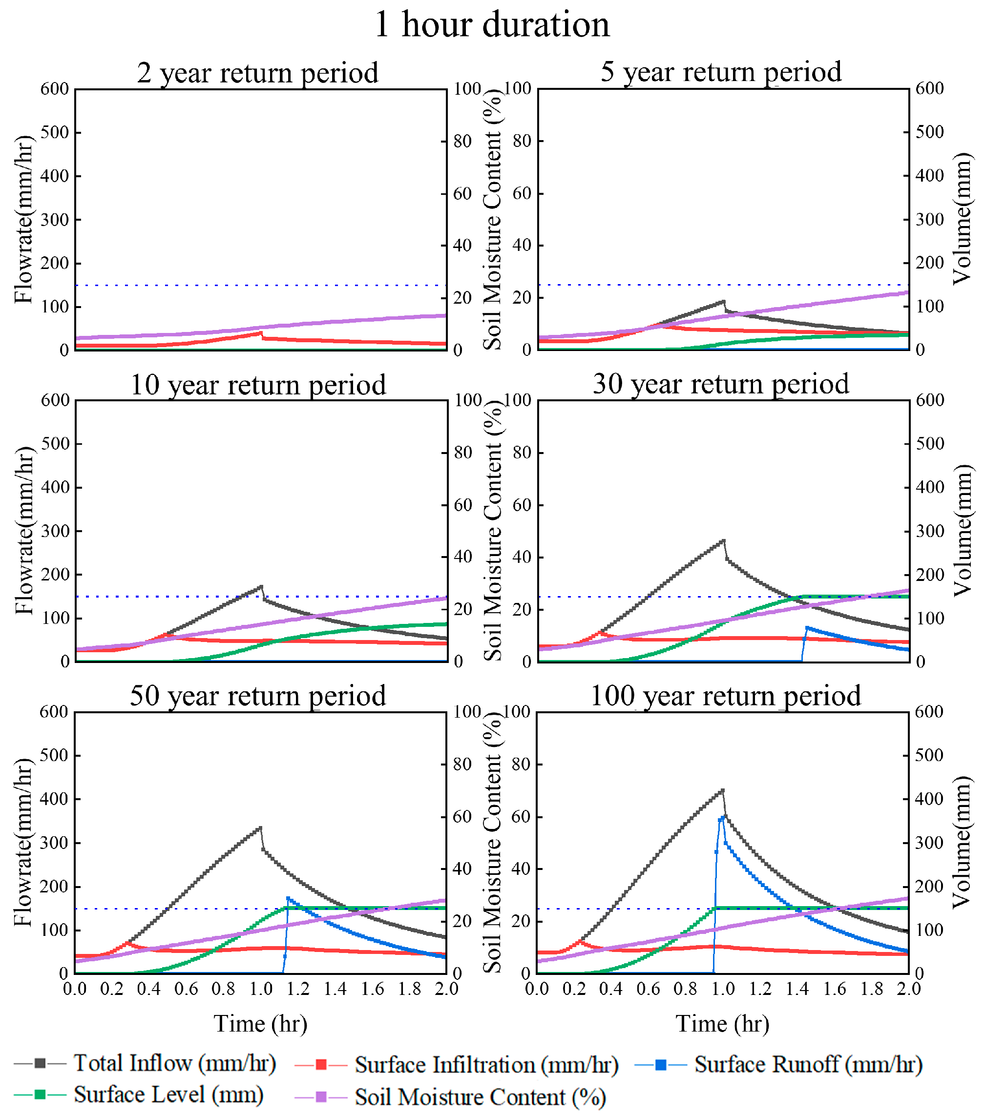
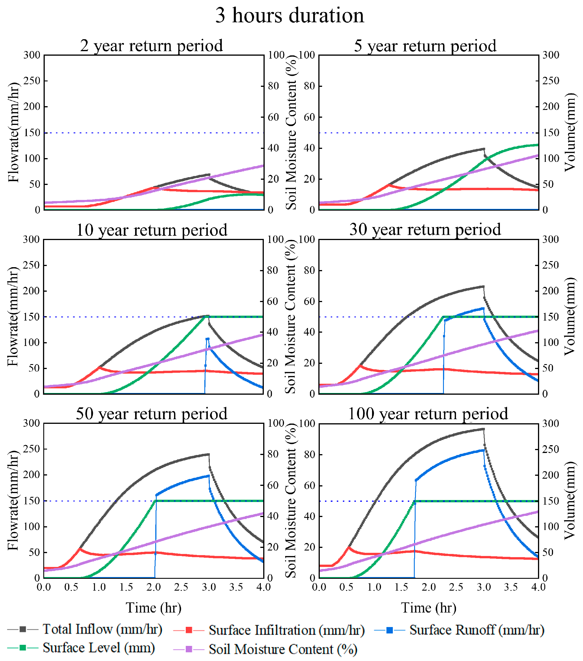
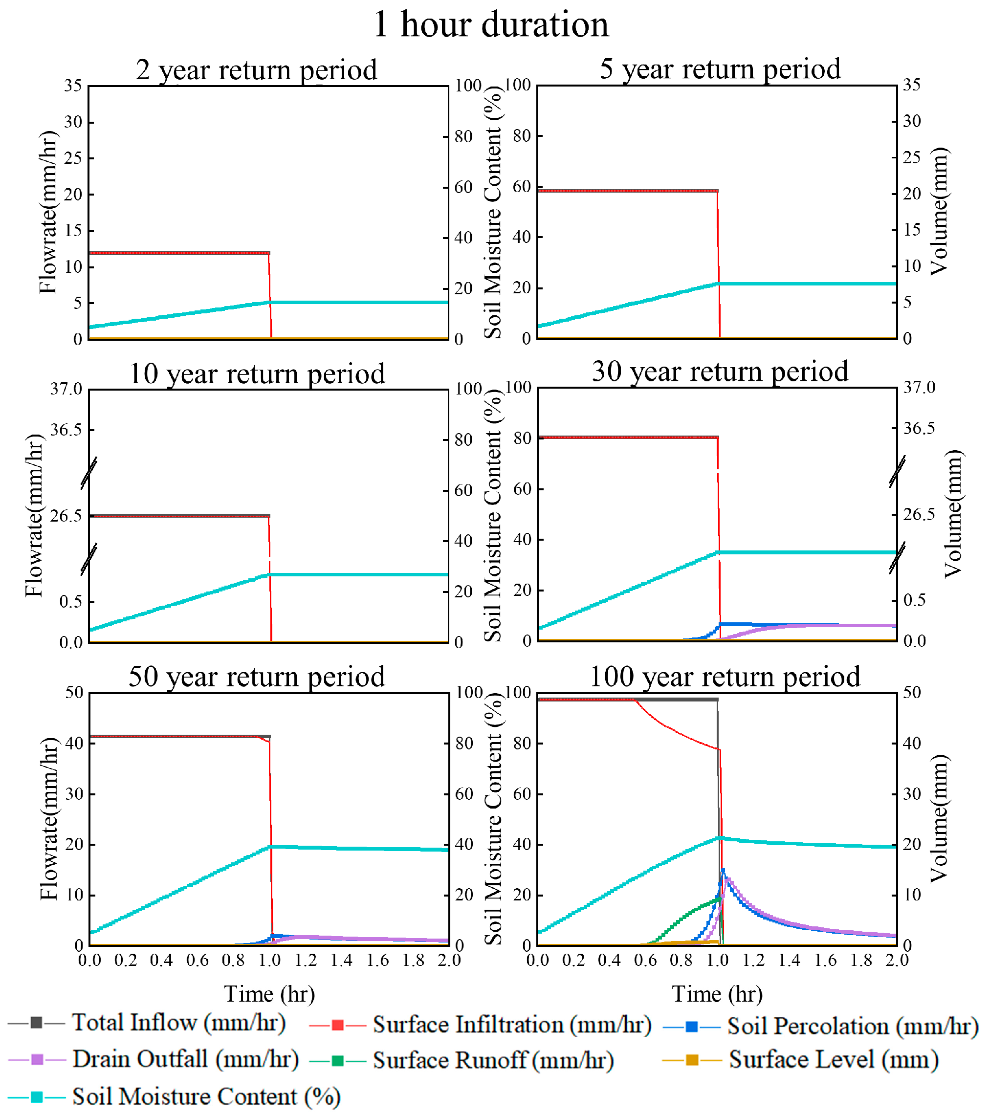
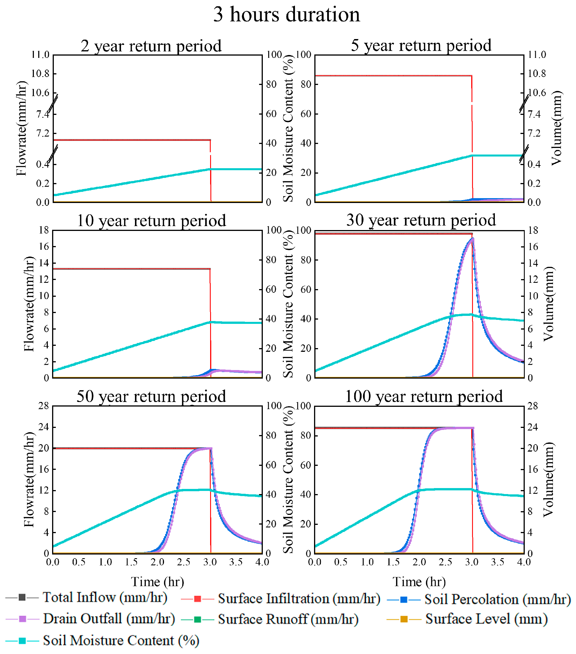
3.1. Effectiveness of SuDS in a Single Catchment

In the first step, we simulated the performance of SuDS components under various rainfall events in a single catchment to determine the physical mechanisms behind the SuDS performance, which could help to understand the performance of SuDS with various spatial distributions. The catchment for this part of the study was a hypothetical catchment that represents the property of the study area. The width of this catchment was estimated by the GIS data, while the other parameters were set to average values of the subcatchments in it. In total, 1149 potential sites (22,980 m²) for SuDS installation, among which 622 sites (12,440 m²) for green roofs and 527 sites (10,540 m²) for rain gardens, were identified and used. Specifications for the representative catchment and applied SuDS are given in

Table 2. Parameter settings of the hypothetical subcatchment in the SWMM model.

Object	Parameter	Value	Unit
Catchment	Area	28.9	ha
	Width	200	m
	Slope	53.4	%
	Percentage of impervious area	54.4	%
	Manning’s n value of impervious areas	0.012	none
	Manning’s n value of pervious areas	0.389	none
	Depression storage of impervious areas	2.54	mm
	Depression storage of pervious areas	5.08	mm
	Proportion of impervious areas with no depression storage	0	%
Rain Garden	Area	10,540	m2
	Percentage of impervious area	100	%
	Surface width per unit	0	m
	Number of SuDS units	527	none
Green Roof	Area	12,440	m2
	Percentage of impervious area	0	%
	Surface width per unit	5	m
	Number of SuDS units	622	none

.

Detailed reports of the SuDS component from the SWMM are helpful to explicate their underlying physical mechanisms. The process data of two SuDS components were compared in 12 rainfall events based on data extracted from SWMM detailed reports. For 1 h and 3 h rainfall events with different return periods, Figure 8 and Figure 9 display the process data that characterize the performance of rain gardens, while Figure 10 and Figure 11 display the process data that characterize the performance of green roofs. The blue dotted horizontal line was added to the figures as an auxiliary line to represent the water storage limit based on a given berm height of 150 mm.

SuDS facilities are commonly designed to reduce discharge runoff by increasing the recharge of subsurface flows and extend the duration of stormwater retention. Rain gardens are infiltration-based SuDS facilities with an engineered soil layer to reduce stormwater runoff and peak flow at the site. As shown in Figure 8, the total inflow sequentially undergoes three processes of infiltration into the soil layer, being stored in the surface space, and generating outflow after the it enters the rain gardens. When the rainfall intensity (mm/h) is lower than the maximum infiltration rate (mm/h) of the surface soil, the total inflow completely infiltrates into the gaps of filler particles in the soil layer and gradually increases the soil moisture content. It can be observed in 5- and 10-year events that when the inflow gradually exceeds the soil infiltration rate over time, rainwater begins to accumulate in the surface storage space formed by the berm, and the surface water level gradually rises. This means the surface storage space provides the rain gardens with storage capacity, and the amount of water retained and the delay time of peak runoff mainly depend on the height of the berms. When the surface water level reaches the berm height after the peak inflow occurs, rain gardens can simultaneously cause a reduction in surface runoff and a delay in the appearance of peak runoff, as shown in the results of 30- and 50-year events. This can be attributed to the accommodation of remaining surface storage space to the peak flow.

As the intensity of the rainfall increases, the surface water level will react more quickly to changes in inflow, thereby reducing the extent of delayed discharge. Regardless of the return period, the results mentioned above can also be observed in Figure 9. By comparing the results of 1 h events and 3 h events over the same return period, rain gardens are more prone to produce surface runoff in the 3 h events. This means that rainfall events with longer duration consume more surface storage capacity, leaving the rain garden with less remaining storage capacity to accommodate the inflow.

Compared to the rain garden, the green roof has a thinner soil layer and an extra drainage mat layer under it to drain rainwater. However, for safety reasons, green roofs are not equipped with berms to create extra storage capacity on the surface like rain gardens. Therefore, as retention-based facilities, the main processes in green roofs to mitigate rainwater are infiltrating into the soil layer, being retained in the soil layer and discharging from the drainage mat. As shown in the results for 2-, 5-, 10- and 30-year events in Figure 10, when the rainfall intensity is low, all rainwater can infiltrate into the soil layer of the green roofs and cause an increase in soil moisture and soil percolation. In this case, percolation in the soil layer starts when the soil moisture reaches the threshold of 24.9%. When analyzing the results of soil percolation in Figure 10 and Figure 11, we found that the threshold (24.3–25.0%) is universal and almost unaffected by rainfall events, and its magnitude is primarily affected by soil characteristics. As shown in the results of 50- and 100-year events, with the gradual increase of soil moisture, the infiltration rate of rainwater in the rain garden suddenly began to decline rapidly, and it began to produce surface runoff. This means that in response to events with high rainfall intensity, the retaining capacity of the soil layer may be quickly exhausted.

Similar results in the rainfall events with a 3 h duration can be observed in Figure 11. When the soil moisture is relatively low and there is enough capacity to retain the rainwater, it can temporarily remain in the soil layer instead of percolating to the drainage mat layer. As the rainfall intensity increases, the time when the rainwater starts to be discharged from the drainage mat gradually advances, and the discharged flow will reach a higher peak. When the accumulation of rainwater in the soil layer makes the soil saturated, the buffering effect of the rain gardens on the peak flow disappears, and the peak flow returns to the level of total inflow.

Our results demonstrate that the surface storage capacity and the rainwater infiltration into the soil layer of the rain gardens are the primary mechanisms that affect the reduction of peak flow and the delayed discharge of surface runoff, while the retention and percolation of rainwater in the soil layer are the main mechanisms that affect the green roof in reducing discharge runoff and delaying the appearance of peak flow. By comparing the results of the two SuDS facilities in 1 h and 3 h events with a 30- to 50-year return period, we also noticed that rain gardens are more sensitive to the accumulated rainfall, while the efficiency of the green roofs is primarily affected by the rainfall intensity. This may be because rain gardens eventually allow infiltration of rainwater into the natural soil to supplement groundwater, while green roofs can discharge rainwater accumulated in the soil layer through the drainage mat layer more quickly.

3.2. The Simulation Results of the SWMM Model

3.2.1. The Total Discharge Volume and Discharge Flow Rate

As shown in Figure 12, the reduction rate of total discharge volume (TDV), average discharge flow rate (ADFR) and maximum discharge flow rate (MDFR) from the downstream outlet of 27 considered scenarios are plotted with the connectedness, edge density and flow distance in scatter diagrams. The solid red line represents the fitting curve of these results.

As shown in Figure 12, the connectedness of green roofs (GRs) and rain gardens (RGs) shows a strong positive linear correlation with TDV, ADFR and MDFR reduction rate in most cases. The results in Figure 12 also show that an increase in connectedness from GR to RG leads to a greater reduction of TDV and ADFR than an increase in connectedness from RG to RG. This suggests that TDV and ADFR reduction rates are more sensitive to increased connectivity between green roofs and rain gardens than to increased connectivity among rain gardens. Moreover, the difference was not affected by the duration and intensity of rainfall events. Based on the analysis of the physical mechanisms of green roofs and rain gardens in flood reduction mentioned in Section 3.1, we believe that increased connectedness can enhance the flood reduction efficiency of rain gardens by increasing the utilization of their remaining surface storage or potential infiltration capacity. As they are connected, rain gardens that have exhausted storage and infiltration capacity can drain the outflow to other rainwater gardens that have remaining storage capacity to avoid direct discharge of rainwater. The connection from green roofs to the rain gardens not only allows the rainwater discharged from the green roofs to be infiltrated again or temporarily stored in rain gardens, but also increases the infiltration time of rainwater in rain gardens through the delayed discharge of the green roofs. This may be one reason why it can achieve better efficiency in reducing TDV and ADFR than increasing the connection of rain gardens.

As shown in Figure 12, the connectedness from green roofs to rain gardens showed a strong linear correlation with the reduction rate of MDFR when facing 3 h events. The reduction of MDFR seems to be more susceptible to connectedness among rain gardens. This may be due to changes in the number of SuDS, which can buffer rainwater at the MDFR site. When no SuDS are connected, the peak flow is mainly affected by the infiltration or temporary storage of rainwater by few SuDS near the MDFR site. When the strategy of connecting green roofs to rain gardens is adopted, both the few green roofs located near the MDFR site and their directly connected rain gardens can buffer peak flows. When rain gardens are also connected, more connected rain gardens can be used to buffer the peak flow at the MDFR site, even though they may not be near the site. However, there was no obvious correlation between green roof connectivity and the reduction in MDFR during 1 h events. This may be because green roofs in scenarios 1 to 5 have already achieved optimal performance in reducing MDFR. This suggests that when facing short-term heavy rainfall events, increased connectedness from green roofs to rain gardens cannot enhance MDFR reduction at the community scale. Furthermore, increased connectedness has a slightly greater effect on the reduction rate of TDV, ADFR and MDFR in 1 h rainfall events than in 3 h rainfall events, both for green roofs and rain gardens.

The results in Figure 13 show that increasing the edge density of rain gardens has a better promoting effect on TDV, ADFR and MDFR reduction than green roofs.

Obviously, as the green roofs become more decentralized from scenario 11 to 14, they can receive a wider range of rainwater and temporarily store it in the soil layer. However, in these scenarios, rain gardens are centrally installed on large green lands, so not all delayed rainwater discharge from green roofs can flow into the rain gardens and be infiltrated or stored. In this case, the increase in the dispersion of green roofs only slightly prompts the reduction rates of TDV, ADFR and MDFR, as shown in the results of increasing GR edge density in Figure 13. On the other hand, the results of increasing RG edge density show that the decentralized distribution of rain gardens can lead to a greater reduction of TDV, ADFR and MDFR. This may be because the decentralized distribution of rain gardens not only increases the receiving range of rainwater, but also receives surface runoff over a larger area. In addition, rainwater received by green roofs is likely to be discharged as free flow for a short period of time, while rainwater received by rain gardens can eventually be infiltrated into the natural soil instead of becoming surface runoff again. Moreover, increasing the edge density of the two SuDS components helps reduce TDV, ADFR and MDFR in 1 h rainfall events slightly more than in 3 h rainfall events. This indicates that the duration and intensity of precipitation events are related to this difference.

In summary, the results demonstrate that the increase of both connectedness and edge density would promote the decrease of TDV, ADFR and MDFR, although the performance of GR and RG is different. For a certain increase in connectedness, GR had greater potential in reducing TDV and ADFR, while RG reduced MDFR. From the perspective of edge density, RG presented a more significant effect than GR in reducing TDV, ADFR and MDFR. The effect of the enhancement of connectedness and edge density on flood reduction performance seems to be more noticeable in 1 h events.

From the aspect of flow distance, Figure 14 demonstrates that flow distance has a fair linear correlation with the reduction of TDV, ADFR and MDFR, except the reduction of MDFR in 1 h events. The linear fitting result between flow distance and reduction of MDFR shows a weak positive linear correlation.

As shown in Figure 14, the reduction rates of TDV and ADFR decrease as rain gardens’ average flow distance increases. This suggests that when rain gardens are installed downstream of surface runoff, they can be more effective in reducing TDV and ADFR. Since the rainfall events in this study are set as spatially uniform precipitation, we believe that the main reason for this difference is the difference in surface runoff flowing into rain gardens. When rain gardens are installed downstream, the higher inflow rate can rapidly increase the rate of rainwater accumulation in the surface storage space of rain gardens and make them discharge earlier. However, as rain gardens only buffer and attenuate the inflow from upstream their installation sites, rain gardens installed downstream can receive and treat inflow from a wider range of surface runoff, resulting in greater TDV and ADFR reduction rates. The effect of increasing flow distance on reducing TDV and ADFR in 1 h events is greater than in 3 h events for rain gardens. This means that the flood reduction effect caused by the location of the rain gardens may be more sensitive to short-term rainfall events.

On the contrary, the fitting results of MDFR reduction rate in Figure 14 present a negative correlation between flow distance and MDFR. Therefore, the reduction rate of MDFR decreases as the installation location of rain gardens shifts from upstream to downstream. As mentioned above, when the rain gardens are installed downstream of surface runoff, the rainwater acquires a large inflow velocity through the accumulation of gravitational potential energy before flowing into the rain gardens. This strategy allows rain gardens to reduce ADFR more effectively, but it also accelerates the depletion of surface storage space. As shown in Figure 8 and Figure 9, when the storage capacity of rain gardens is exhausted before peak flow occurs, there is some time for discharge runoff to accumulate kinetic energy and reach the MDFR. Therefore, the reduction rate of MDFR will decrease as the time to speed up the discharge flow rate increases.

Among these 27 scenarios, the SuDS components in scenario 18 achieved the greatest reduction of TDV, ADFR and MDFR, except scenario 17 achieved the greatest reduction of MDFR in a 3 h rainfall event.

3.2.2. The Changes of Discharge Flow Rate in Downstream Outlet Versus Time

According to the time series results reported by SWMM, the scatter charts are plotted to illustrate the variation trend of discharge flow rate (DFR) in the considered simulation process, as shown in Figure 15 and Figure 16.

As shown in Figure 15a,b and Figure 16a,b, the flow rate curve of Sc-0 and Sc-1 share a similar variation trend, but with different values. The discharge flow rate in both scenarios increases sharply as the rainfall event starts and then climbs to the maximum DFR. This means that installing unconnected SuDS at the community scale can reduce the discharge flow rate but has limited buffering effect on the rapid rising of DFR at the beginning of the rainfall event. As the connectivity of SuDS components in Sc-2 to Sc-9 increases, the sharp increasing trend of DFR at the beginning of 1 h events becomes a slower increasing trend. The results in Figure 15a,b show that GR connectivity could mitigate the increasing trend of DFR from 6 to 40 min since the beginning of rainfall, while RG connectivity tends to mitigate the increasing trend of DFR from 40 to 60 min. As shown in the results of scenario 9 in Figure 15, when all rain gardens and green roofs were connected, SuDS achieved the best DFR reduction among Sc-1 to Sc-9. Similar results can also be observed in scatter graphs in Figure 16a,b. When facing 3 h events, GR connectivity can reduce the increasing trend of DFR from 10 to 80 min since the beginning of the rainfall, while RG connectivity tends to reduce the increasing trend of DFR from 50 to 180 min. Compared to the green roofs, the rain garden’s surface storage capacity composed of berms helps to buffer the inflow during high flow rates and increases the infiltration time. This suggests that increasing GR connectivity can improve the mitigation efficiency of SuDS against runoff with a low flow rate, while increasing RG connectivity can help reduce inflow with a high flow rate.

Comparing the results in Figure 15c,d and Figure 16c,d, respectively, the edge density of rain gardens has a more significant effect on slowing down the rise of DFR than that of green roofs. In 1 h events, the increase of the edge density of RG can more effectively reduce the DFR during rainfall, including the peak discharge flow rate. In the 3 h event, the increase in the edge density of RG obviously leads to a less significant reduction of the peak discharge flow rate. This may be due to the exhausted infiltration and storage capacity of rain gardens before the peak flow appears, caused by the longer rainfall duration. Although the mitigation effect of flow distance is not as notable as for connectedness and edge density, its increase changes the upper concave, increasing the curve to a lower concave one, as shown in Figure 15e. Similar variation trends can also be seen in the 3 h rainfall event, as shown in Figure 16. This can be attributed to the fact that the rain gardens installed downstream can receive more runoff from the upstream region, thus increasing their chances of storing and absorbing surface runoff. The maximum discharge flow rate in the whole rainfall event in 28 scenarios including Sc-0 appears after the rain stops for 1 min. However, the delay in maximum flow rate is not observed.

3.3. The Simulation Results of the HiPIMS Model

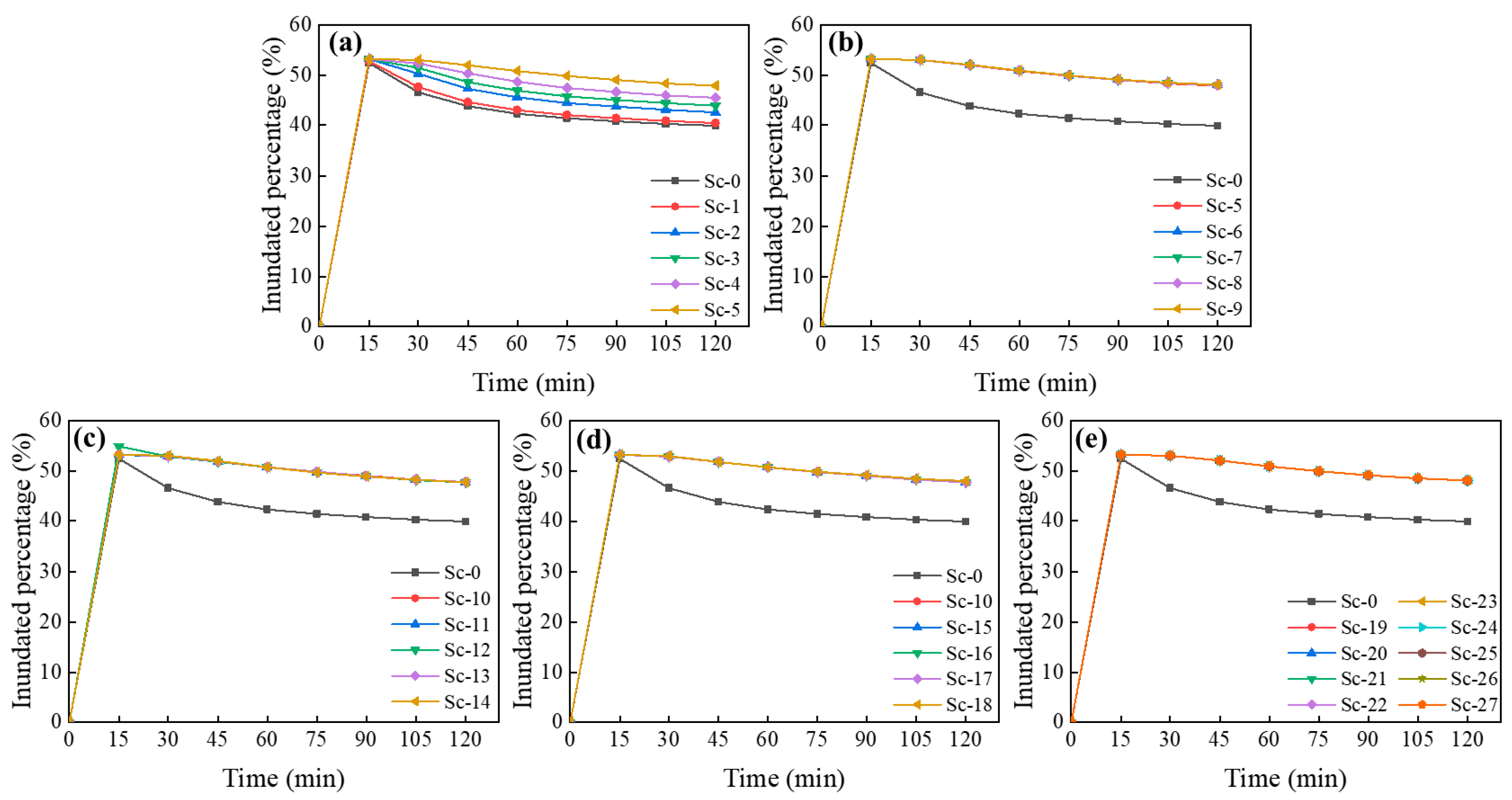
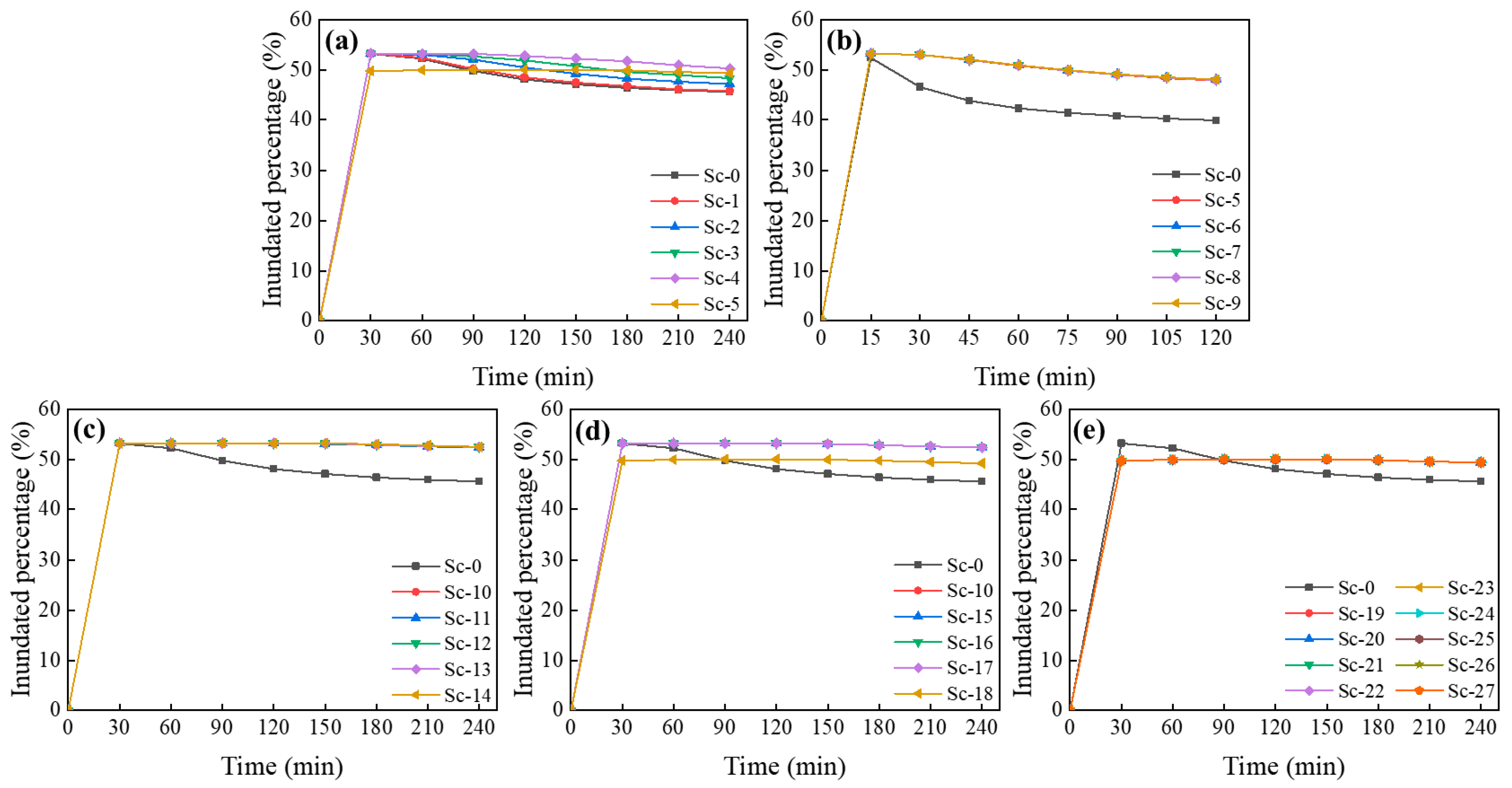
3.3.1. The Proportion of the Inundated Areas

According to the time series results reported by Hi-PIMS, the line graphs are plotted to illustrate the variation trend of the inundated area (IA) in the considered simulation process, as shown in Figure 17 and Figure 18.

As shown in Figure 17a–e, the increase of connectivity between SuDS components can lead to the increase of the inundated percentage, while the edge density and flow distance have almost no effect on it. The results of Sc-0 in Figure 17 show the variation trend of the inundated area without SuDS. With the beginning of the rainfall, the inundated percentage in the study area first increases rapidly and then decreases gradually, because surface runoff under the influence of gravity will converge to lower places and cause the decrease of the inundated area. The rainwater convergence is also accompanied by an increase in the inundated depth at the converging sites. Thus, despite causing an expansion of the inundated area, the implementation of SuDS can delay and slow the convergence of surface runoff and the formation of deep inundated sites, which is also supported by the results shown in Figure 19 and Figure 20. Moreover, the results in Figure 17a,b indicate that the inundated area in the study area gradually expands with the increase of connectivity from green roofs to rain gardens. However, increasing the connectivity among rain gardens on this basis has no effect on the change of the inundated area. Similar results can also be observed in Figure 18. Interestingly, as green roofs are increasingly connected to rain gardens, we observe less inundated area between 0 and 90 min in Sc-5 than in Sc-0 in 3 h events. This means that in the low-intensity rainfall events, improved connectivity has the potential to reduce the inundated area for a certain time since the beginning of rainfall.

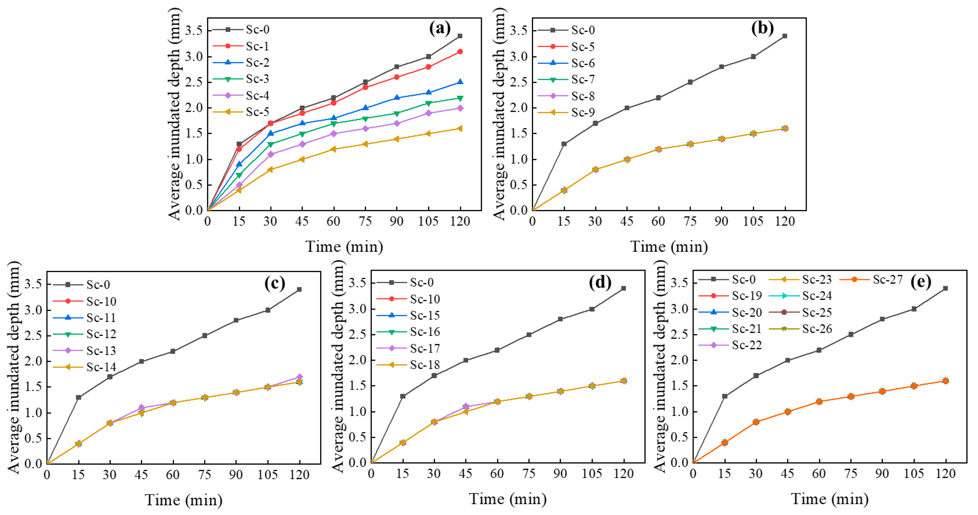
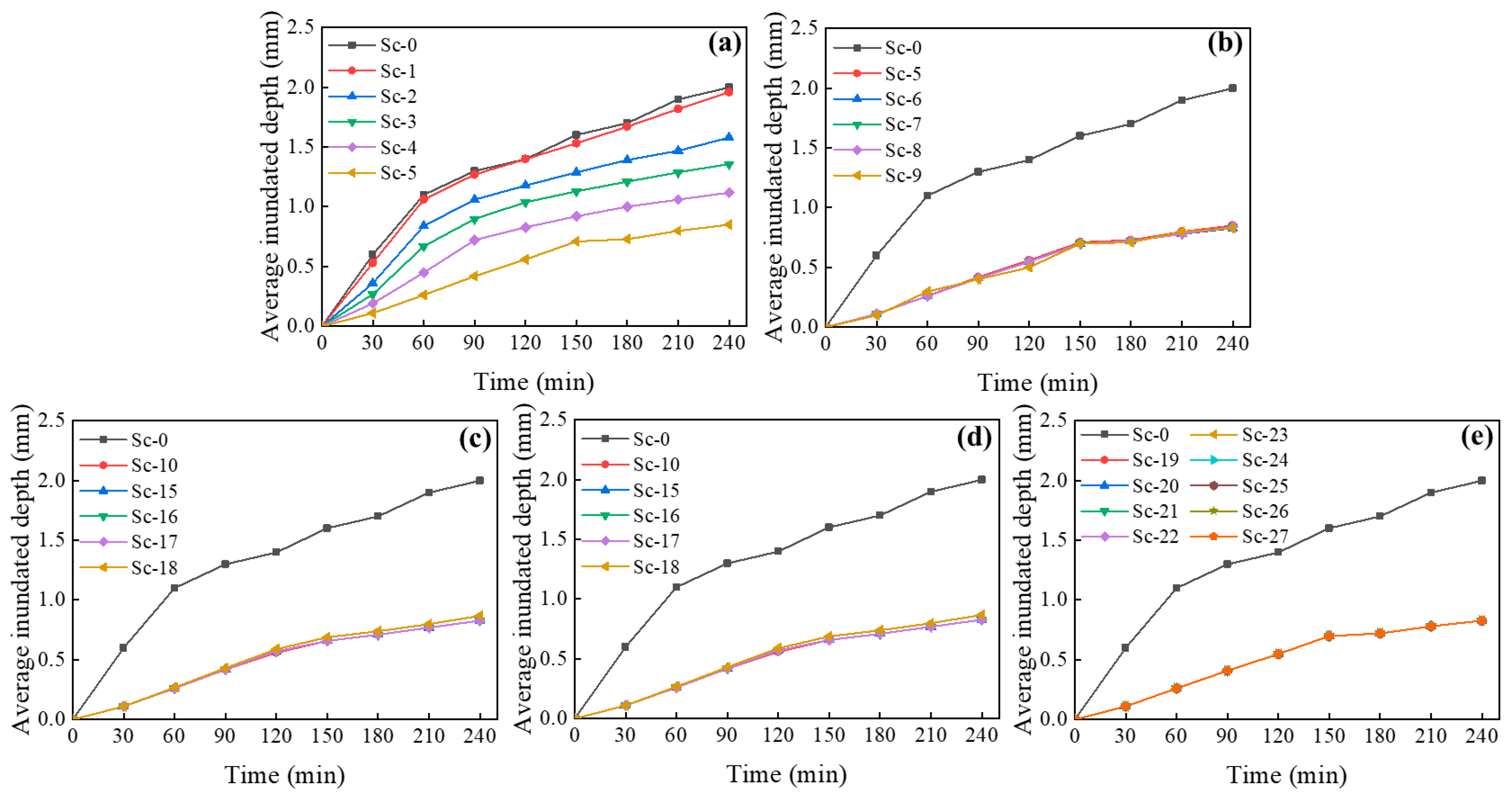
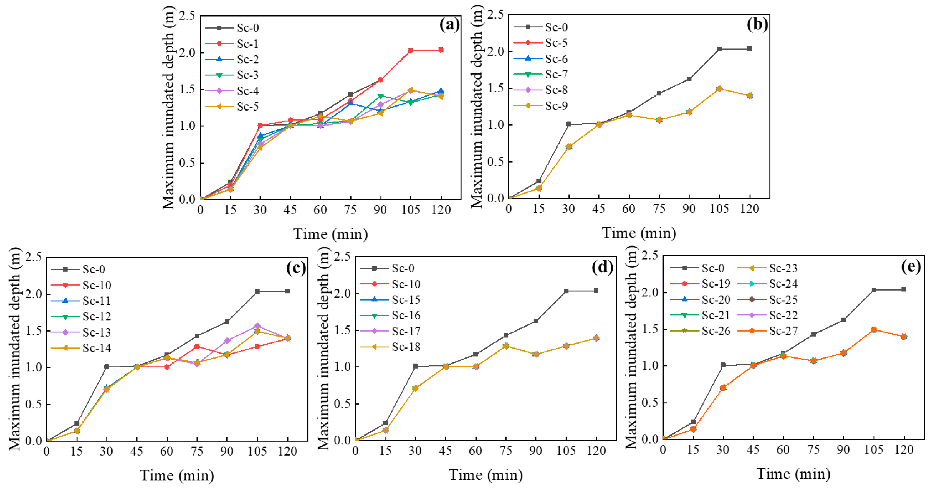
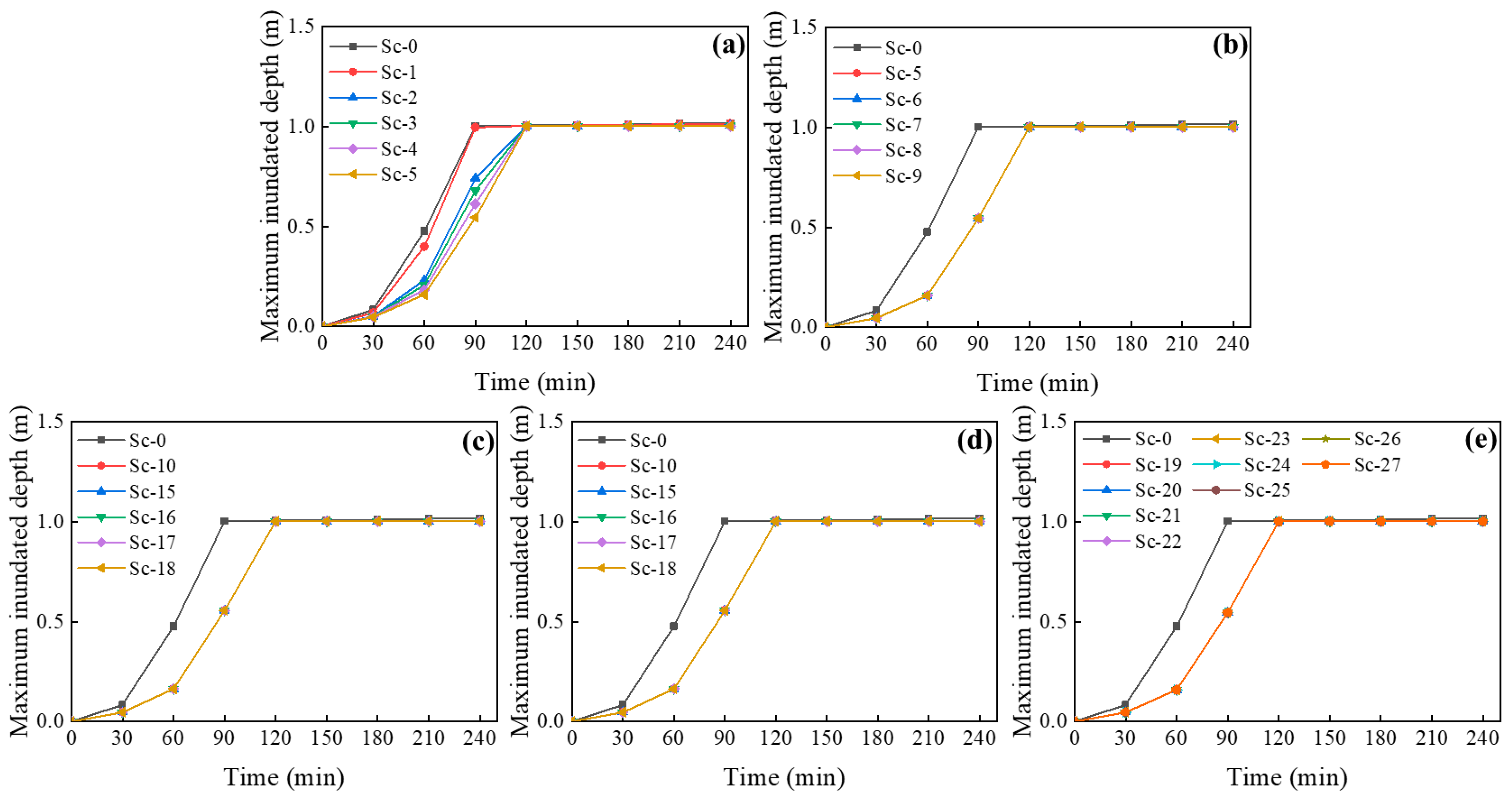
3.3.2. The Inundation Depth of the Study Area

According to the time series results reported by HiPIMS, the line graphs are plotted to illustrate the variation trend of average inundated depth (AID) and maximum inundated depth (MID) in the considered simulation process, as shown in Figure 19.

The results in Figure 19a,b and Figure 20a,b show that increased connectedness from green roofs to rain gardens significantly results in a decrease in the average inundated depth, while increased connectedness among rain gardens hardly reduces the average inundated depth. This means that connecting green roofs to rain gardens is a more efficient way to reduce the average inundated depth than increasing connectivity among rain gardens.

As shown in Figure 19c,d and Figure 20c,d, the increase of green roofs’ edge density has a slight contribution to the decrease of AID. This means that decentralized green roofs can reduce the average inundated depth better at the community scale. Interestingly, the increase in the edge density of the rain garden can slightly contribute to the decrease in the AID during the 1 h event, but may cause a slight increase in the AID during the 3 h event. These results suggest that the effect of decentralized rain gardens on AID may be reversed with increasing duration of rainfall events. Moreover, the results in Figure 19e and Figure 20e show that flow distance has no effect on the efficiency of the rain gardens in reducing AID.

The results in Figure 21a,b show that with the increase of connectedness from green roofs to rain gardens, the maximum inundation depth in the study area shows a decreasing trend between 0 and 45 min in 1 h rainfall events. However, GR connectivity has little correlation with the MID from 45 to 120 min of the rainfall event. By examining the map of inundated depth distribution for 1 h events as reported by HI-PIMS, we found that the location and depth of the MID after 45 min changed with the progress of the rainfall. Therefore, we speculate that the variation of MID after 45 min may be more affected by its location and topographic conditions. This indicates that when the rainfall intensity is high, due to the impact of topographic factors, increasing the connectivity of rain gardens may not always achieve a stable effect of MID reduction. Similar results are observed in Figure 22. The results of graphs (a)–(c) show that the MID decreases significantly with the increase of green roof connectivity during 0–120 min of a 3 h rainfall event, and its correlation with green roof connectivity begins to weaken after 120 min. This difference may be related to the saturation of green roofs’ soil layer and the depletion of rain gardens’ surface storage. By examining the map of inundated depth distribution, we also find that the MID in 3 h events always appears at a certain location in the sub-catchment S10 during the rainfall process. This indicates that the connectivity from green roofs to rain gardens is positively correlated with the decrease of MID when its appearance location is steady. However, in both 1 h and 3 h events, increased connectivity among rain gardens cannot reduce the maximum inundated depth.

As shown in Figure 21c,d and Figure 22c,d, although the effect of the increase of GR edge density on the reduction of MID is not obvious in 1 h rainfall events, this effect was clearly observed in the results of 3 h rainfall events. This indicates that when the location of the maximum inundation depth does not change with the rainfall process, the increase of the GR edge density contributes to the decrease of the MID. However, the increased edge density of rain gardens does not affect the MID of the study area in both 1 h and 3 h events. Meanwhile, the results in Figure 21e and Figure 22e also indicate that the flow distance of the rain gardens has no effect on reducing the maximum inundation depth. Interestingly, we find that the spatial distribution of rain gardens (indicated by connectedness, edge density and flow distance) does not seem to affect the inundated depth. However, this does not mean that changing the spatial distribution of green roofs is a more effective way of reducing the MID than changing the spatial distribution of rain gardens. Considering that the location where the MID appears is always in the sub-catchment S10, the inconspicuous effect of rain gardens on MID may be due to the small area of sub-catchment S10. The lack of potential installation location for rain gardens could be the main reason why MID is not sensitive to the change of their connectivity, edge density and flow distance.

4. Discussion

In terms of the impact of the spatial distribution of SuDS components on their flood reduction performance, there is currently a lack of a general guide and recommendations to support the spatial distribution design of SuDS components, especially at the community scale. According to the SuDS design process provided in the SuDS manual, the spatial distribution design of SuDS components should proceed in the outline design stage [25]. However, as for the specific design of the spatial distribution of SuDS components at the community scale, only nine urban typologies are provided in the SuDS manual as design examples [25]. These typologies cannot cover all the complex contexts in different communities, especially old ones.

Based on the understanding of the primary flood reduction mechanisms of green roofs and rain gardens, we analyzed the effect of spatial distribution characteristics (connectivity, decentralization and position along flow direction) of green roofs and rain gardens at the community scale on flood reduction performance (TDV, ADFR, MDFR, and increasing trend of DFR, IA, AID and MID) of SuDS systems. Increased connectivity can effectively increase the reduction rates of TDV, ADFR and MDFR, mainly because the delayed discharge of rainwater from green roofs and the sharing of surface storage capacity among rain gardens helps to increase the time for rainwater to be retained and infiltrate, thus increasing the infiltration and reducing runoff flow rate. Previous studies have shown that connectivity between SuDS components can effectively reduce peak runoff in mesoscale and macroscale catchments such as cities and watersheds [33,35], while our results suggest that increased connectivity can also improve the flood reduction performance of SuDS at the community scale. In our study, the decentralized level is increased under the premise that SuDS is connected. So, as the decentralized level of SuDS components increases, they can receive surface runoff inflows from a larger area of subcatchments, thus more effectively buffering and reducing TDV, ADFR and MDFR at the community scale. Previous studies have indicated that decentralized SuDS can better reduce peak runoff when facing small rainfall events (total precipitation <27 mm) at the urban scale than clustered SuDS, while the clustered SuDS performs better in large rainfall events (total precipitation >27 mm) [34]. Therefore, decentralized distribution strategies can promote the flood reduction performance of SuDS at both urban and community scales in small rainfall events. The results of our study further indicate that at the community scale, decentralized SuDS components still have better performance than clustered SuDS when faced with large rainfall events with total precipitation of 36.39 mm and 52.81 mm. Our study demonstrates that the effect of location of rain gardens along the flow direction on their flood reduction at the community scale is mainly attributed to the difference of inflow. When rain gardens are installed downstream, their flood reduction potential can be better exploited to reduce TDV and ADFR, because surface runoff from a larger area can be received. However, downstream installation also means that it will receive inflows with greater flow rates, which may cause the rain garden’s infiltration capacity and surface storage to saturate before the peak flow occurs, resulting in an increase in MDFR. However, a previous study showed that concentrated retention ponds and permeable pavements in the middle stream can better reduce peak runoff at the community scale [37]. The different results may be due to the use of different SuDS components. Since the selected SuDS components in our study (rain garden and green roof) do not depend on underground storage layers, our results can better provide theoretical support for the design of SuDS spatial distribution in communities with high groundwater levels.

Previous studies mostly used peak runoff and discharge volume as the main indicators to study SuDS performance [36,37], while our study also focused on the response of inundated depth and inundated area to different spatial distribution strategies of SuDS, providing a more comprehensive evaluation. As shown in the time series diagram of DFR under different scenarios, the increase of GR connectivity contributes to the reduction of DFR at the beginning of rainfall, while the reduction of DFR in the middle and late of rainfall is mainly affected by RG connectivity. This may be because rainwater entering green roofs could be temporarily retained and the discharge delayed. Then, the discharged rainwater begins to infiltrate into the soil layers of rain gardens. Furthermore, the IA is positively affected by the connectivity from GR to RG when facing rainfall events, whereas the AID will decrease as the connectivity increases. The reason is that increased connectivity from GR to RG can facilitate rainwater retention and infiltration in both SuDS components to reduce the AID more efficiently. By examining the flood maps in the Supplementary Materials, we find that the MID in 1 h events does not decrease as the connectivity increases, which may be due to the irregularly change of the MID occurrence location. In the simulations of 3 h events where MID location does not change, the obvious positive correlation between increased connectivity and reduced MID can also prove this point. However, it is not clear why IA, AID and MID are not sensitive to the changes of connectivity, decentralized level and flow distance of rain gardens. One possible hypothesis is that areas that remain inundated after SuDS are implemented may lack potential installation sites for rain gardens.

5. Conclusions

This study aims to explore the relationship between different spatial distribution scenarios of sustainable urban drainage systems (SuDS) and the flood reduction performance at a community scale. Using the stormwater management model (SWMM) and the high-performance integrated hydrodynamic modelling system (HI-PIMS), different spatial distributions scenarios of rain gardens and green roofs at the community scale were simulated in a community in the Kensington and Chelsea Royal District (RBKC), west London, UK. The 27 design scenarios consider different connectivity, decentralized level, and SuDS component locations along the flow direction. Each scenario was simulated in 1 h and 3 h rainfall events with a 30-year return period.

The total discharge volume (TDV), average discharge flow rate (ADFR) and maximum discharge flow rate (MDFR) of the 27 considered scenarios were plotted and fitted with the connectedness, edge density and flow distance. We also plotted the scatter charts and line graphs to illustrate the variation trend of discharge flow rate (DFR), inundated area (IA), average inundated depth (AID) and maximum inundated depth (MID) in the considered simulation process. These results demonstrate that SuDS would have the best comprehensive performance in the studied community-scale catchment when applying connected and decentralized distribution strategies.

Specifically, the connectivity between SuDS components had a positive correlation with the TDV, ADFR, and MDFR in short-term rainfall events. It was also revealed that the positive correlation only existed between the connectivity from green roofs to rain gardens and the reduction of AID and MID. The connectivity of green roofs to rain gardens also had a negative effect on the reduction of IA. However, the connectivity of rain gardens had no correlation with IA, AID and MID. The increased connectivity of GR could slow down the increasing trend of DFR at the beginning of the rainfall event, while the increased connectivity of RG could mitigate the increasing trend of DFR at the middle and late periods.

On the other hand, the decentralized level of SuDS components had a positive correlation with the reduction of TDV, ADFR and MDFR in short-term rainfall events. However, the positive correlation only existed between the decentralized level of green roofs and the mitigation of AID and MID, while the decentralized level of rain gardens had no correlation with IA, AID and MID. The increase of the decentralized level of green roofs had no effect on the inundated area. The increase of the decentralized level of rain gardens could slow down the increasing trend of DFR more efficiently than that of green roofs during the rainfall events.

As for the position of rain gardens along the flow direction, opposite effects on the indicators of flood events were observed in the simulation results. The upstream installation of rain gardens along the flow direction had the best performance on the reduction of TDV and ADFR at community scale, whereas the downstream installation strategy had the best performance on the reduction of MDFR and the mitigation of the increasing trend of DFR. The flow distance of SuDS components presented no correlation with IA, AID and MID.

This paper will contribute to the improvement of the spatial distribution design process of SuDS at a community scale by contributing to the general design guidelines. Our findings demonstrate the effect of SuDS components’ connectivity, decentralized level and position along the flow direction on their flood reduction performance through seven indicators (the reduction rate of TDV, ADFR, MDFR, IA, AID, MID, and the mitigation of the increasing trend of DFR). These findings will improve the guidelines and support the work of designers in a more universal way, especially when the local contexts do not match the nine typologies of the SuDS manual very well.

This paper also reveals the possible mechanisms of spatial distribution affecting the flood reduction performance of SuDS components based on the analysis of hydrological processes. We believe that connectivity improves the efficiency of buffering and mitigating the effects of heavy rain primarily through the coupling of green roofs with rain gardens and sharing of surface storage capacity among rain gardens. The contribution of decentralized level to flood reduction performance can be attributed to the fact that the decentralized SuDS components can receive rainwater and surface runoff from a larger area. The different locations of rain gardens along the flow direction mainly affect the inflow characteristics of surface runoff. For example, rain gardens located downstream receive inflow with high flow rate, while rain gardens located upstream receive runoff flow with low flow rate. However, further research is needed to explore the principles of spatial distribution affecting the performance of SuDS components through the combined use of model simulation and in situ experiments.

References

1. Wheater, H.S. Flood Hazard and Management: A UK Perspective. Philos. Trans. R. Soc. A Math. Phys. Eng. Sci. 2006, 364, 2135–2145. [Google Scholar] [CrossRef] [PubMed]
2. Yin, J.; Yu, D.; Yin, Z.; Liu, M.; He, Q. Evaluating the Impact and Risk of Pluvial Flash Flood on Intra-Urban Road Network: A Case Study in the City Center of Shanghai, China. J. Hydrol. 2016, 537, 138–145. [Google Scholar] [CrossRef] [Green Version]
3. Maskrey, S.A.; Mount, N.J.; Thorne, C.R. Doing flood risk modelling differently: Evaluating the potential for participatory techniques to broaden flood risk management decision-making. J. Flood Risk Manag. 2022, 15, e12757. [Google Scholar] [CrossRef]
4. Mahmood, M.I.; Elagib, N.A.; Horn, F.; Saad, S.A.G. Lessons Learned from Khartoum Flash Flood Impacts: An Integrated Assessment. Sci. Total Environ. 2017, 601, 1031–1045. [Google Scholar] [CrossRef]
5. Jiang, Y.; Zevenbergen, C.; Ma, Y. Urban Pluvial Flooding and Stormwater Management: A Contemporary Review of China’s Challenges and “Sponge Cities” Strategy. Environ. Sci. Policy 2018, 80, 132–143. [Google Scholar] [CrossRef]
6. Zhou, Q.; Leng, G.; Huang, M. Impacts of Future Climate Change on Urban Flood Volumes in Hohhot in Northern China: Benefits of Climate Change Mitigation and Adaptations. Hydrol. Earth Syst. Sci. 2018, 22, 305–316. [Google Scholar] [CrossRef] [Green Version]
7. EM-DAT The International Disaster Database. Available online: https://www.emdat.be/ (accessed on 16 June 2020).
8. Burak, S.; Doǧan, E.; Gazioǧlu, C. Impact of Urbanization and Tourism on Coastal Environment. Ocean Coast. Manag. 2004, 47, 515–527. [Google Scholar] [CrossRef]
9. Klein, R.D. Urbanization and Stream Quality Impairment. J. Am. Water Resour. Assoc. 1979, 15, 948–963. [Google Scholar] [CrossRef]
10. Liu, Z.; Wang, Y.; Li, Z.; Peng, J. Impervious Surface Impact on Water Quality in the Process of Rapid Urbanization in Shenzhen, China. Environ. Earth Sci. 2013, 68, 2365–2373. [Google Scholar] [CrossRef]
11. Skougaard Kaspersen, P.; Høegh Ravn, N.; Arnbjerg-Nielsen, K.; Madsen, H.; Drews, M. Comparison of the Impacts of Urban Development and Climate Change on Exposing European Cities to Pluvial Flooding. Hydrol. Earth Syst. Sci. 2017, 21, 4131–4147. [Google Scholar] [CrossRef] [Green Version]
12. Arnone, E.; Pumo, D.; Francipane, A.; La Loggia, G.; Noto, L.V. The Role of Urban Growth, Climate Change, and Their Interplay in Altering Runoff Extremes. Hydrol. Process. 2018, 32, 1755–1770. [Google Scholar] [CrossRef]
13. Zhou, Q.; Leng, G.; Su, J.; Ren, Y. Comparison of Urbanization and Climate Change Impacts on Urban Flood Volumes: Importance of Urban Planning and Drainage Adaptation. Sci. Total Environ. 2019, 658, 24–33. [Google Scholar] [CrossRef] [PubMed]
14. Barbosa, A.E.; Fernandes, J.N.; David, L.M. Key Issues for Sustainable Urban Stormwater Management. Water Res. 2012, 46, 6787–6798. [Google Scholar] [CrossRef] [PubMed]
15. Burns, M.J.; Fletcher, T.D.; Walsh, C.J.; Ladson, A.R.; Hatt, B.E. Hydrologic Shortcomings of Conventional Urban Stormwater Management and Opportunities for Reform. Landsc. Urban Plan. 2012, 105, 230–240. [Google Scholar] [CrossRef]
16. Miller, J.D.; Hutchins, M. The Impacts of Urbanisation and Climate Change on Urban Flooding and Urban Water Quality: A Review of the Evidence Concerning the United Kingdom. J. Hydrol. Reg. Stud. 2017, 12, 345–362. [Google Scholar] [CrossRef] [Green Version]
17. Jung, I.W.; Chang, H.; Moradkhani, H. Quantifying Uncertainty in Urban Flooding Analysis Considering Hydro-Climatic Projection and Urban Development Effects. Hydrol. Earth Syst. Sci. 2011, 15, 617–633. [Google Scholar] [CrossRef] [Green Version]
18. Mahmoud, S.H.; Gan, T.Y. Urbanization and Climate Change Implications in Flood Risk Management: Developing an Efficient Decision Support System for Flood Susceptibility Mapping. Sci. Total Environ. 2018, 636, 152–167. [Google Scholar] [CrossRef]
19. Wu, X.; Wang, Z.; Guo, S.; Liao, W.; Zeng, Z.; Chen, X. Scenario-Based Projections of Future Urban Inundation within a Coupled Hydrodynamic Model Framework: A Case Study in Dongguan City, China. J. Hydrol. 2017, 547, 428–442. [Google Scholar] [CrossRef]
20. Chan, F.K.S.; Yang, L.E.; Scheffran, J.; Mitchell, G.; Adekola, O.; Griffiths, J.; Chen, Y.; Li, G.; Lu, X.; Qi, Y.; et al. Urban flood risks and emerging challenges in a Chinese delta: The case of the Pearl River Delta. Environ. Sci. Policy 2021, 122, 101–115. [Google Scholar] [CrossRef]
21. Won, Y.-M.; Lee, J.-H.; Moon, H.-T.; Moon, Y.-I. Development and Application of an Urban Flood Forecasting and Warning Process to Reduce Urban Flood Damage: A Case Study of Dorim River Basin, Seoul. Water 2022, 14, 187. [Google Scholar] [CrossRef]
22. Dieperink, C.; Mees, H.; Priest, S.J.; Ek, k.; Bruzzone, S.; Larrue, C.; Matczak, P. Managing Urban Flood Resilience as a Multilevel Governance Challenge: An Analysis of Required Multilevel Coordination Mechanisms. Ecol. Soc. 2018, 23, 230131. [Google Scholar] [CrossRef]
23. Munawar, H.S.; Khan, S.I.; Anum, N.; Qadir, Z.; Kouzani, A.Z.; Parvez Mahmud, M.A. Post-Flood Risk Management and Resilience Building Practices: A Case Study. Appl. Sci. 2021, 11, 4823. [Google Scholar] [CrossRef]
24. Fletcher, T.D.; Shuster, W.; Hunt, W.F.; Ashley, R.; Butler, D.; Arthur, S.; Trowsdale, S.; Barraud, S.; Semadeni-Davies, A.; Bertrand-Krajewski, J.-L.; et al. SUDS, LID, BMPs, WSUD and More—The Evolution and Application of Terminology Surrounding Urban Drainage. Urban Water J. 2015, 12, 525–542. [Google Scholar] [CrossRef]
25. Ballard, B.W.; Wilson, S.; Udale-Clarke, H.; Illman, S.; Scott, T.; Ashley, R.; Kellagher, R. The SuDS Manual; Department for Environment Food & Rural Affairs: London, UK, 2015; pp. 1–964. [Google Scholar]
26. Maqbool, R.; Wood, H. Containing a sustainable urbanized environment through SuDS devices in management trains. Sci. Total Environ. 2022, 807, 150812. [Google Scholar] [CrossRef]
27. Seyedashraf, O.; Bottacin-Busolin, A.; Harou, J.J. Many-Objective Optimization of Sustainable Drainage Systems in Urban Areas with Different Surface Slopes. Water Resour. Manag. 2021, 35, 2449–2464. [Google Scholar] [CrossRef]
28. Jato-Espino, D.; Toro-Huertas, E.I.; Güereca, L.P. Lifecycle sustainability assessment for the comparison of traditional and sustainable drainage systems. Sci. Total Environ. 2022, 817, 152959. [Google Scholar] [CrossRef]
29. Zahmatkesh, Z.; Burian, S.J.; Karamouz, M.; Tavakol-Davani, H.; Goharian, E. Low-Impact Development Practices to Mitigate Climate Change Effects on Urban Stormwater Runoff: Case Study of New York City. J. Irrig. Drain. Eng. 2015, 141, 04014043. [Google Scholar] [CrossRef]
30. Bedan, E.S.; Clausen, J.C. Stormwater Runoff Quality and Quantity from Traditional and Low Impact Development Watersheds. J. Am. Water Resour. Assoc. 2009, 45, 998–1008. [Google Scholar] [CrossRef]
31. Hou, J.; Mao, H.; Li, J.; Sun, S. Spatial Simulation of the Ecological Processes of Stormwater for Sponge Cities. J. Environ. Manag. 2019, 232, 574–583. [Google Scholar] [CrossRef]
32. Zubelzu, S.; Rodríguez-Sinobas, L.; Andrés-Domenech, I.; Castillo-Rodríguez, J.T.; Perales-Momparler, S. Design of Water Reuse Storage Facilities in Sustainable Urban Drainage Systems from a Volumetric Water Balance Perspective. Sci. Total Environ. 2019, 663, 133–143. [Google Scholar] [CrossRef]
33. Haghighatafshar, S.; Jansen, J.L.C.; Aspegren, H.; Jönsson, K. Conceptualization and Schematization of Mesoscale Sustainable Drainage Systems: A Full-Scale Study. Water 2018, 10, 1041. [Google Scholar] [CrossRef] [Green Version]
34. Loperfido, J.V.; Noe, G.B.; Jarnagin, S.T.; Hogan, D.M. Effects of Distributed and Centralized Stormwater Best Management Practices and Land Cover on Urban Stream Hydrology at the Catchment Scale. J. Hydrol. 2014, 519, 2584–2595. [Google Scholar] [CrossRef]
35. Kim, H.W.; Park, Y. Urban Green Infrastructure and Local Flooding: The Impact of Landscape Patterns on Peak Runoff in Four Texas MSAs. Appl. Geogr. 2016, 77, 72–81. [Google Scholar] [CrossRef]
36. Mejia, A.I.; Moglen, G.E. Impact of the Spatial Distribution of Imperviousness on the Hydrologic Response of an Urbanizing Basin. Hydrol. Process. 2010, 24, 3359–3373. [Google Scholar] [CrossRef]
37. Liang, C.Y.; You, G.J.Y.; Lee, H.Y. Investigating the Effectiveness and Optimal Spatial Arrangement of Low Impact Development Facilities. J. Hydrol. 2019, 577, 124008. [Google Scholar] [CrossRef]
38. Chen, P.Y.; Tung, C.P.; Li, Y.H. Low Impact Development Planning and Adaptation Decision-Making under Climate Change for a Community against Pluvial Flooding. Water 2017, 9, 756. [Google Scholar] [CrossRef] [Green Version]
39. Kong, F.; Ban, Y.; Yin, H.; James, P.; Dronova, I. Modeling Stormwater Management at the City District Level in Response to Changes in Land Use and Low Impact Development. Environ. Model. Softw. 2017, 95, 132–142. [Google Scholar] [CrossRef]
40. Zeng, S.; Guo, H.; Dong, X. Understanding the Synergistic Effect between LID Facility and Drainage Network: With a Comprehensive Perspective. J. Environ. Manag. 2019, 246, 849–859. [Google Scholar] [CrossRef]
41. Eckart, K.; Mcphee, Z.; Bolisetti, T. Performance and Implementation of Low Impact Development—A Review. Sci. Total Environ. 2017, 607, 413–432. [Google Scholar] [CrossRef]
42. Johnson, R.D.; Sample, D.J. Environmental Modelling & Software A Semi-Distributed Model for Locating Stormwater Best Management Practices in Coastal Environments. Environ. Model. Softw. 2017, 91, 70–86. [Google Scholar] [CrossRef] [Green Version]
43. Joyce, J.; Chang, N.B.; Harji, R.; Ruppert, T.; Imen, S. Developing a Multi-Scale Modeling System for Resilience Assessment of Green-Grey Drainage Infrastructures under Climate Change and Sea Level Rise Impact. Environ. Model. Softw. 2017, 90, 1–26. [Google Scholar] [CrossRef]
44. Johnson, D.; Geisendorf, S. Are Neighborhood-Level SUDS Worth It? An Assessment of the Economic Value of Sustainable Urban Drainage System Scenarios Using Cost-Benefit Analyses. Ecol. Econ. 2019, 158, 194–205. [Google Scholar] [CrossRef]
45. Guo, R.; Ding, Y.; Shang, L.; Wang, D.; Cao, X.; Wang, S.; Bonatz, N.; Wang, L. Sustainability-Oriented Urban Renewal and Low-Impact Development Applications in China: Case Study of Yangpu District, Shanghai. J. Sustain. Water Built Environ. 2018, 4, 5017006. [Google Scholar] [CrossRef]
46. Latifi, M.; Rakhshandehroo, G.; Nikoo, M.R.; Sadegh, M. A Game Theoretical Low Impact Development Optimization Model for Urban Storm Water Management. J. Clean. Prod. 2019, 241, 118323. [Google Scholar] [CrossRef]
47. Kaykhosravi, S.; Abogadil, K.; Khan, U.T.; Jadidi, M.A. The Low-Impact Development Demand Index: A New Approach to Identifying Locations for LID. Water 2019, 11, 2341. [Google Scholar] [CrossRef] [Green Version]
48. Martin-Mikle, C.J.; De Beurs, K.M.; Julian, J.P.; Mayer, P.M. Identifying Priority Sites for Low Impact Development (LID) in a Mixed-Use Watershed. Landsc. Urban Plan. 2015, 140, 29–41. [Google Scholar] [CrossRef] [Green Version]
49. Hou, J.; Zhu, M.; Wang, Y.; Sun, S. Optimal Spatial Priority Scheme of Urban LID-BMPs under Different Investment Periods. Landsc. Urban Plan. 2020, 202, 103858. [Google Scholar] [CrossRef]
50. Jia, H.; Yao, H.; Tang, Y.; Yu, S.L.; Zhen, J.X.; Lu, Y. Development of a Multi-Criteria Index Ranking System for Urban Runoff Best Management Practices (BMPs) Selection. Environ. Monit. Assess. 2013, 185, 7915–7933. [Google Scholar] [CrossRef]
51. Yin, D.; Evans, B.; Wang, Q.; Chen, Z.; Jia, H.; Chen, A.S.; Fu, G.; Ahmad, S.; Leng, L. Integrated 1D and 2D Model for Better Assessing Runoff Quantity Control of Low Impact Development Facilities on Community Scale. Sci. Total Environ. 2020, 720, 137630. [Google Scholar] [CrossRef]
52. Cai, Y.; Lin, X.; Yue, W.; Zhang, P. Inexact Fuzzy Chance-Constrained Programming for Community-Scale Urban Stormwater Management. J. Clean. Prod. 2018, 182, 937–945. [Google Scholar] [CrossRef]
53. Zellner, M.; Massey, D.; Minor, E.; Gonzalez-Meler, M. Exploring the Effects of Green Infrastructure Placement on Neighborhood-Level Flooding via Spatially Explicit Simulations. Comput. Environ. Urban Syst. 2016, 59, 116–128. [Google Scholar] [CrossRef] [Green Version]
54. Meerow, S.; Newell, J.P. Spatial Planning for Multifunctional Green Infrastructure: Growing Resilience in Detroit. Landsc. Urban Plan. 2017, 159, 62–75. [Google Scholar] [CrossRef]
55. Defra Data Service Platform. Available online: https://environment.data.gov.uk/DefraDataDownload/?Mode=survey (accessed on 15 August 2020).
56. Flood Risk Maps for Surface Water in England—December 2019. Available online: https://environment.maps.arcgis.com/apps/MapSeries/index.html?appid=bfe44552ba1849d594de7b40fdcfa685# (accessed on 14 August 2020).
57. Rossman, L.A. Storm Water Management Model User’s Manual Version 5.1; National Risk Management Research Laboratory; Office of Research and Development; U.S. Environmental Protection Agency: Cincinnati, OH, USA, 2015; pp. 1–327. [Google Scholar]
58. Soilscapes—Cranfield Soil and Agrifood Institute. Available online: http://www.landis.org.uk/soilscapes/index.cfm (accessed on 15 August 2020).
59. Faulkner, D. Flood Estimation Handbook 2: Rainfall Frequency Estimation; Centre for Ecology & Hydrology: Oxford, UK, 2008; pp. 1–110. [Google Scholar]
60. Flood Estimation Handbook Web Service. Available online: https://fehweb.ceh.ac.uk/ (accessed on 15 August 2020).
61. Xia, X.; Liang, Q.; Ming, X. A Full-Scale Fluvial Flood Modelling Framework Based on a High-Performance Integrated Hydrodynamic Modelling System (HiPIMS). Adv. Water Resour. 2019, 132, 103392. [Google Scholar] [CrossRef]
Figure 1. The DSM map of the study area in RBKC, west London, England [55].
Water 14 01367 g001
Figure 2. The flood risk map for surface water in the study area in RBKC, west London, England [56].
Water 14 01367 g002
Figure 3. The land use map of the study area: blue polygons represent buildings; green polygons represent green land; pink polygons represent open space; yellow polygons represent roads.
Water 14 01367 g003
Figure 4. The subcatchments and drainage system in the study area: red points represent nodes; blue point represents outlet; thick solid blue lines represent pipelines; yellow polygons represent roads; pink polygons represent subcatchments; blue arrows represent flow direction in the pipelines.
Water 14 01367 g004
Figure 5. Sketch maps of different connection strategies. In scenario 1, neither RG or GR is connected; scenario 5, 526 GRs are connected to nearby RGs; scenario 9, 526 GRs are connected to nearby RGs and 422 RGs are connected to nearby RGs.
Water 14 01367 g005
Figure 6. Sketch maps of different decentralized strategies. In scenario 10, 622 GR units are clustered in 69 mini-catchments and 527 RG units are clustered in 18 mini-catchments; scenario 14, 622 GR units are decentralized in 622 mini-catchments and 527 RG units are clustered in 18 mini-catchments; scenario 18, 622 GR units are clustered in 69 mini-catchments and 527 RG units are decentralized in 527 mini-catchments.
Water 14 01367 g006
Figure 7. Sketch maps of different position strategies. In scenario 19, RGs are applied in upstream mini-catchments along flow direction; scenario 23, RGs are applied in even-numbered mini-catchments along flow direction; scenario 27, RGs are applied in downstream mini-catchments along flow direction.
Water 14 01367 g007
Figure 8. SWMM detailed reports on rain gardens in 1 h rainfall events.
Water 14 01367 g008
Figure 9. SWMM detailed reports on rain gardens in 3 h rainfall events.
Water 14 01367 g009
Figure 10. SWMM detailed reports on green roofs in 1 h rainfall events.
Water 14 01367 g010
Figure 11. SWMM detailed reports on green roofs in 3 h rainfall events.
Water 14 01367 g011
Figure 12. Effect of connectivity of SuDS components on TDV, ADFR and MDFR: (a) GR to RG, in 1 h event; (b) RG to RG, in 1 h event; (c) GR to RG, in 3 h event; (d) RG to RG, in 3 h event.
Water 14 01367 g012
Figure 13. Effect of decentralized level of SuDS components on TDV, ADFR and MDFR: (a) GR, in 1 h event; (b) RG, in 1 h event; (c) GR, in 3 h event; (d) RG, in 3 h event.
Water 14 01367 g013
Figure 14. Effect of rain gardens’ position along the flow direction on TDV, ADFR and MDFR: (a) 1 h rainfall event; (b) 3 h rainfall event.
Water 14 01367 g014
Figure 15. The time series plot of DFR in 1 h event in considered scenarios of (a) connectedness of GR; (b) connectedness of RG; (c) edge density of GR; (d) edge density of RG; (e) flow distance of RG.
Water 14 01367 g015
Figure 16. The time series plot of DFR in 3 h event in considered scenarios of (a) connectedness of GR; (b) connectedness of RG; (c) edge density of GR; (d) edge density of RG; (e) flow distance of RG.
Water 14 01367 g016
Figure 17. The time series plot of IA in 1 h event in considered scenarios of (a) connectedness of GR; (b) connectedness of RG; (c) edge density of GR; (d) edge density of RG; (e) flow distance of RG.
Water 14 01367 g017
Figure 18. The time series plot of IA in 3 h event in considered scenarios of (a) connectedness of GR; (b) connectedness of RG; (c) edge density of GR; (d) edge density of RG; (e) flow distance of RG.
Water 14 01367 g018
Figure 19. The time series plot of AID in 3 h event in considered scenarios of (a) connectedness of GR; (b) connectedness of RG; (c) edge density of GR; (d) edge density of RG; (e) flow distance of RG.
Water 14 01367 g019
Figure 20. The time series plot of AID in 3 h event in considered scenarios of (a) connectedness of GR; (b) connectedness of RG; (c) edge density of GR; (d) edge density of RG; (e) flow distance of RG.
Water 14 01367 g020
Figure 21. The time series plot of MID in 3 h event in considered scenarios of (a) connectedness of GR; (b) connectedness of RG; (c) edge density of GR; (d) edge density of RG; (e) flow distance of RG.
Water 14 01367 g021
Figure 22. The time series plot of MID in 3 h event in considered scenarios of (a) connectedness of GR; (b) connectedness of RG; (c) edge density of GR; (d) edge density of RG; (e) flow distance of RG.
Water 14 01367 g022