
The Marine Influence Index (MII): A Tool to Assess Estuarine Intertidal Mudflat Environments for the Purpose of Foraminiferal Biomonitoring


Abstract
:1. Environmental Biomonitoring in Coastal Marine Ecosystems
- (1)
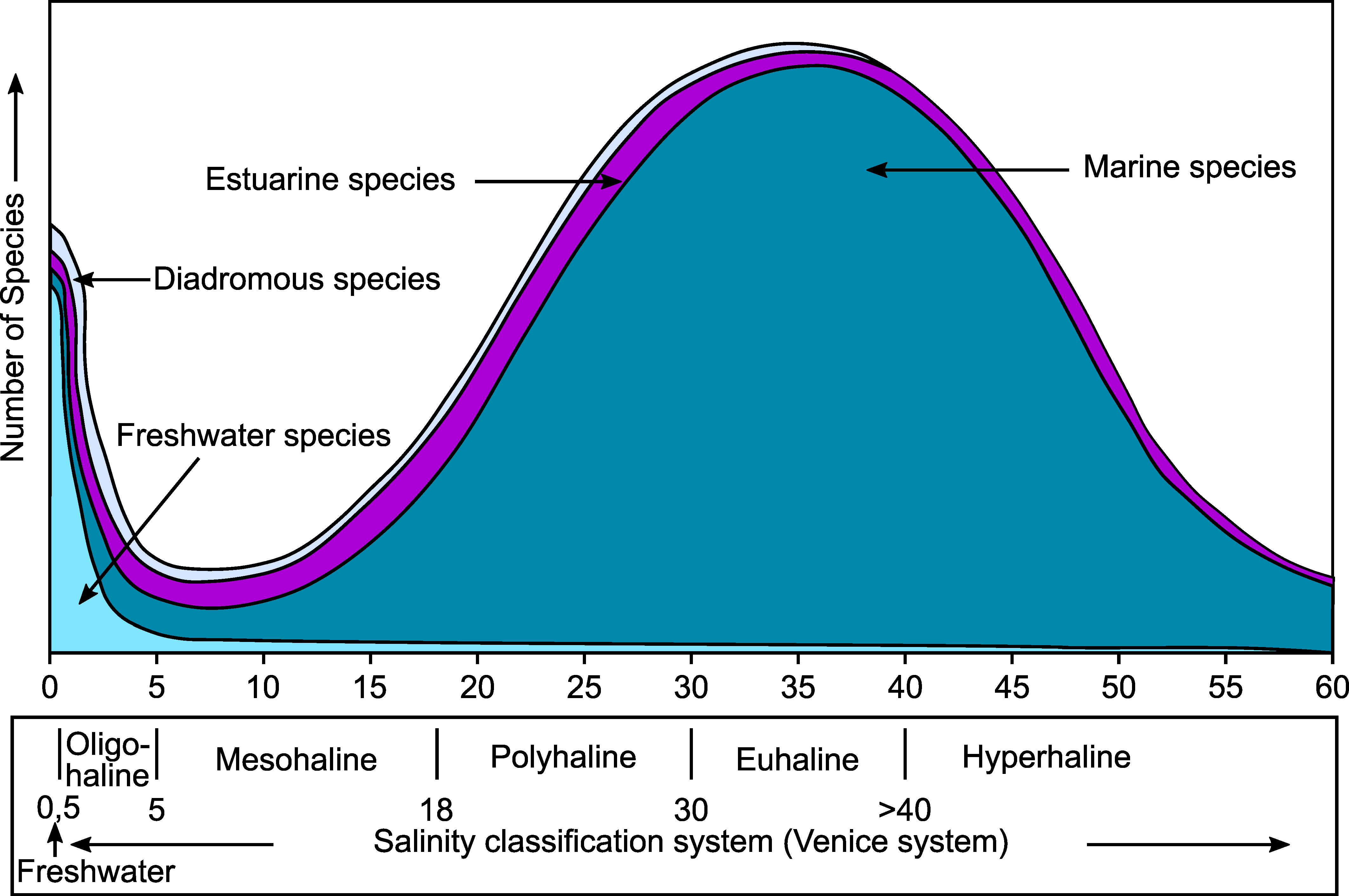
- The presence of a strong salinity gradient, from fully marine conditions at the mouth of the estuary, to brackish and freshwater in the inner part of the estuary. Few species can cope with such a huge salinity range. Most marine and freshwater species are stenohaline and can only bear minor salinity changes. It appears that estuaries are mainly inhabited by some more euryhaline marine species, whereas strictly estuarine species, living exclusively within estuaries, are rare or even non-existent [27,28];
- (2)
- Many environmental parameters show a high spatial and temporal variability. This is the case for salinity, which may show a huge variability on a seasonal (due to the changes in river discharge), as well as daily (weather forcing), and hourly (tidal cycles) scale. In intertidal areas, also other important ecological parameters (such as temperature, evaporation, resources, predation pressure, etc.) may vary dramatically spatially (e.g., due to different emersion times), seasonally, or even during a single tidal cycle.
2. Factors Controlling Faunal Distribution in Estuaries
3. Ecology of Estuarine Foraminifera
- Tidal influence will diminish with increasing distance from the sea and will vary along the lunar-solar tidal cycles. The tides largely control the estuarine circulation and the associated biological processes. The hydrodynamics of the rising and falling tide generates turbulence and causes vertical mixing between fresh and marine waters. Depending on the local tidal regime, river discharge, and the morphology of the estuary, estuaries may be weakly to strongly stratified. The seasonal changes in river discharge and the dynamics of the salt-wedge intrusion also affect biological production [27]. For example, in a seasonally stratified estuary, the presence of the salt wedge in spring led to increased nutrient recycling and phytoplankton blooms [49]. The tidal range will, together with the elevation of the study site, also determine the emergence time of the various parts of the tidal flats;
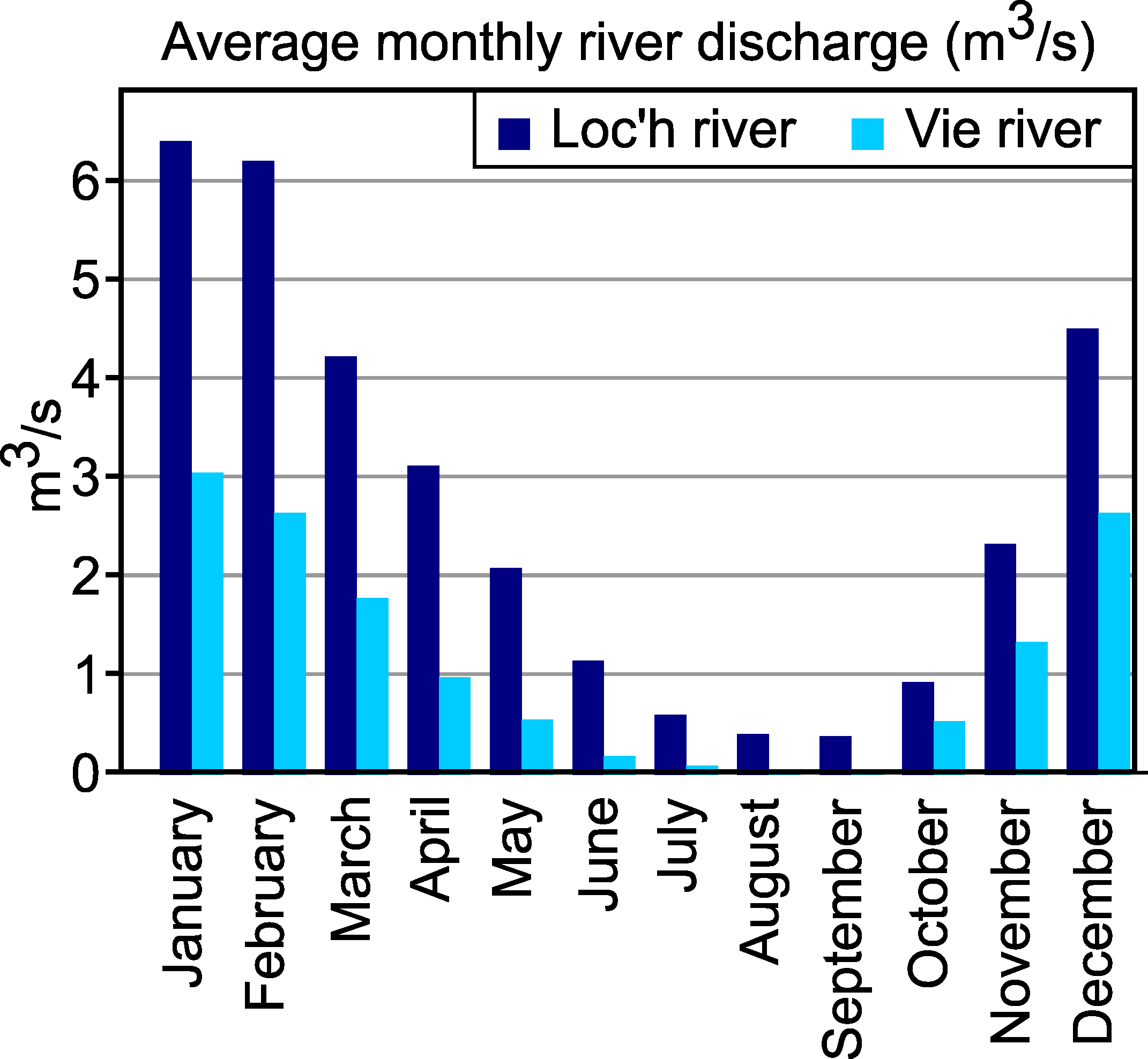
- River discharge, that dilutes the sea water intruding by tidal processes into the estuary, may show major seasonal and interannual variability, depending on the climate regime. Consequently, the sites that are located in the inner estuary may show major seasonal salinity changes, from almost-marine to almost-freshwater;
- Local precipitation is a second source of fresh water, which will especially affect the salinity of the emerged mudflats during low tide;
- Groundwater inflow may be an important additional source of fresh water, which is often difficult to estimate;
- The morphology of the estuary may facilitate or hamper the propagation of the tidal wave and/or of the marine waters in the estuary.
4. Quantifying the Main Parameters Controlling Foraminiferal Distribution in Estuarine Intertidal Mudflats
4.1. Position of the Sampling Point along the Salinity Gradient
- (1)
- Turtuosity: Sea water will have more difficulty entering a meandering estuarine channel than a rectilinear estuary, especially in the case of a strongly curved shape of the channel. For this reason, we propose to measure the relative position of the sampling point with respect to the real distance from the inlet, considering all of the eventual curves of the main channel (i.e., definition of X in Equation (1);
- (2)
- Abrupt narrowing of the estuary or channel sills: Narrowing, or sills of geological origin, will cause major constraints for salt water supplies to the upper parts of the estuary. Such “bottlenecks” will accentuate the non-linearity of the horizontal salinity gradient, and thereby shorten the length of the salt intrusion (i.e., S in Equation (1)). This factor, which is difficult to quantify, should be at least partly integrated in the decrease in marine influence with relative increasing distance from the mouth of the estuary;
- (3)
- Manmade physical obstacles: On the French Atlantic coast, many of the small and medium sized estuaries are closed upstream by a dam provided with a sluice. These dams/sluices are used to prevent salt water from intruding into the fluvial estuary beyond these dams. They are generally closed during rising tides in order to protect fields that are under cultivation from soil salinization. They open during some of the falling tides in order to regulate the outflow of riverine freshwater into the estuary. This is done to keep fluvial waters available for irrigation purposes or to flush the lower parts of the estuary, to remove clay deposits in the navigation channel. When the dam/sluice is closed, the salinity tends to be elevated until the dam is reached, with freshwater being present immediately landward of the dam. As a result, these dams artificially limit the salt intrusion, truncating abruptly the salinity gradient from marine to freshwater. In such cases, we think that the (theoretical) natural salt intrusion should be used to define the relative position of the sampling point on the salinity gradient, and not the observed salt intrusion (until the mechanical obstacle). This natural salt intrusion (before the instalment of the manmade barrier) can be assessed by a careful study of the thalweg topography; normally salt water enters the estuarine valley until the point where the relief starts to increase, often abruptly.
4.2. Altitude/Emergence Time
- (1)
- The elevation of a site may change the position of the foraminiferal assemblage with respect to the vertical salinity gradient, due to haline stratification. In highly stratified estuaries, the salt-water wedge enters the estuary below the outflowing superficial freshwater layer. If present, this vertical gradient will change on diurnal and seasonal timescales in response to incoming and outgoing tide, and to fluctuations in river discharge. Precipitation may be a secondary reason for the development of a vertical salinity gradient, even in the case of estuaries with a homogenized water column. Whatever the exact reasons and salinity values, at higher elevation, the foraminiferal fauna will generally be confronted with lower salinity;
- (2)
- In combination with the tidal range, the elevation largely influences the time of emergence at low tide. The twice-daily emergence of the tidal mudflats exposes the intertidal habitats to major changes of moisture, temperature, and salinity (due to evaporation and/or precipitation). In fact, in the intertidal realm, the time of emergence seems to be a much more important stress factor than slight salinity changes due to the different positions of the sampling sites on the vertical salinity gradient. For macrofauna, emergence also leads to changes in predation pressure, as the contribution of fish decreases while predation by shore-birds and mud-snails becomes more important [59]. Little information is available for predation on foraminifera [60], although there are indications for selective predation by gastropods [61]. Together, these changes represent a substantial recurrent stress;
- (3)
- Hydrodynamic energy will progressively diminish from the estuarine channel to the most elevated parts of the intertidal mudflats. The tidal currents may displace foraminiferal fauna, leading to an underrepresentation of small species and introduction of allochthonous taxa in the intertidal realm. Hydrodynamics will also control sediment grain size and organic matter availability (as organic particles are preferentially bound to clays).
4.3. Importance of Fluvial Discharge
4.4. Distance from the Main Estuarine Channel
5. Defining the Marine Influence Index (MII) for Estuarine Intertidal Mudflats
- X = real distance from the sampling site to the mouth of the estuary, following the main estuarine channel. X is measured between the mouth of the estuary and a line starting from the sampling site, perpendicular to the channel axis.
- S = distance of the natural salt intrusion into the estuary; the observed value when no obstacle is present, a theoretical value based on the thalweg topography when a manmade obstacle is present.
- ET = emergence time, expressed as a fraction of a tidal cycle, calculated for mean spring tide conditions (in France: tidal coefficient 90).
- RD = river discharge in the 30 days before sampling (in m3 s−1).
- CS = surface area of the estuarine cross-section at high tide (in m2).
- Details about the calculation of S, ET and RD/CS are given in the Supplementary Materials.
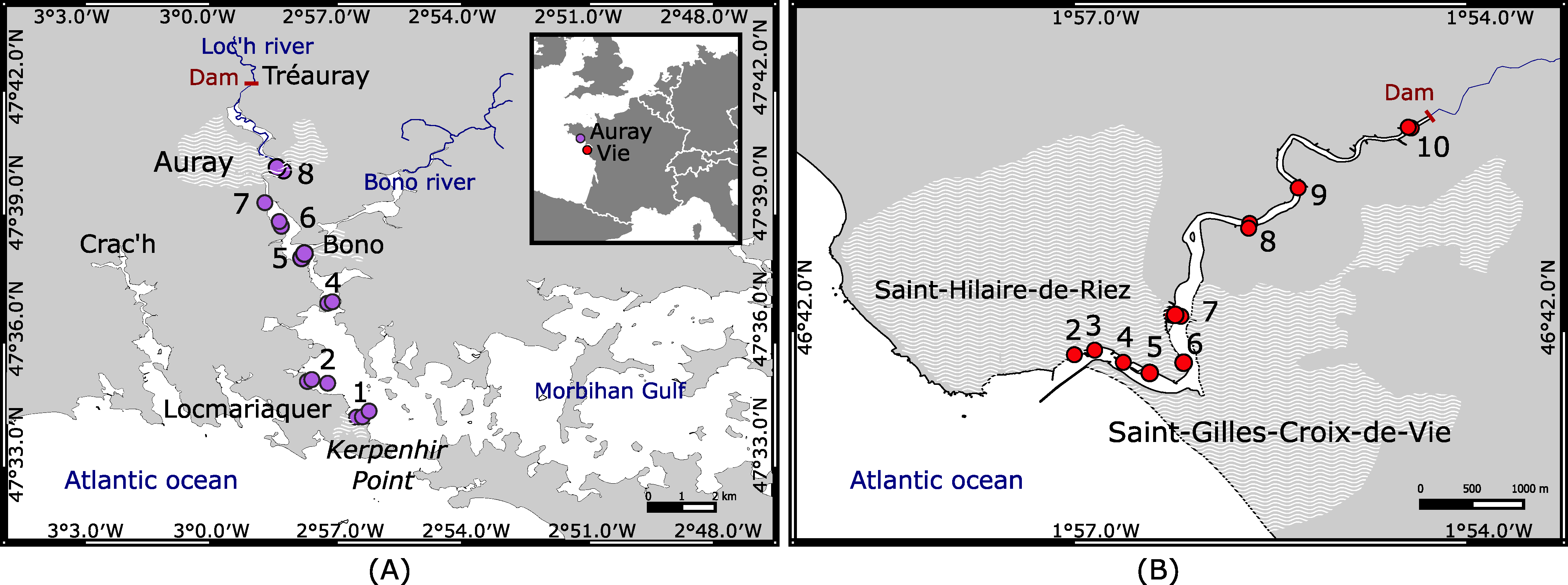
6. Applying the Marine Influence Index (MII) to the Auray and Vie Intertidal Estuarine Mudflats
6.1. Auray Estuary
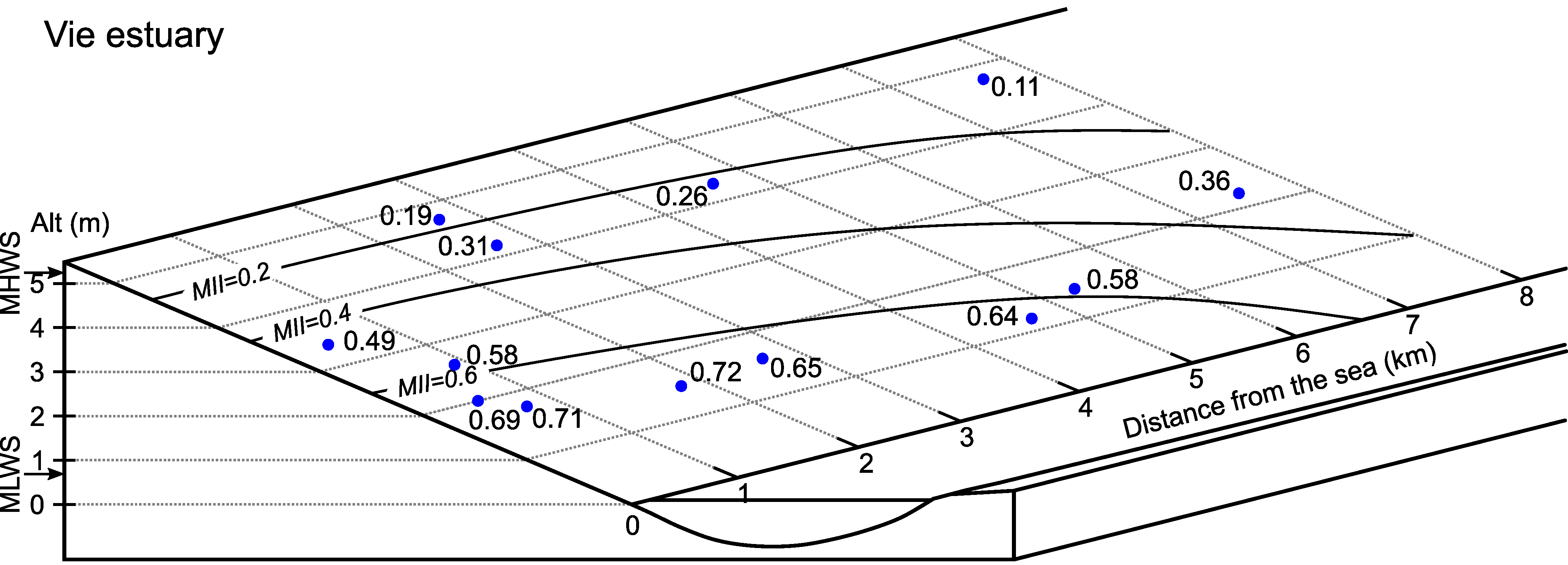
6.2. Vie Estuary
6.3. Comparison of the Two Estuaries, Impact of Seasonal Variation of River Discharge
7. Discussion and Conclusions
- (1)
- The relative position of the sampling point on the gradient between fully marine water and freshwater;
- (2)
- The relative emergence time of the sampling point at the mean spring tide conditions, expressed a percentage of the total length of a tidal cycle. This parameter is closely related to the absolute altitude (with respect to the level of the lowest astronomical tide) of the sampling point;
- (3)
- The relative importance of freshwater outflow, which is determined by dividing the average discharge volume in the 30 days before sampling by the cross-section area of the estuary at each sampling point.
Supplementary Materials
Author Contributions
Funding
Acknowledgments
Conflicts of Interest
References
- United Nations Factsheet: People and Oceans; United Nations: New York, NY, USA, 2017; p. 7. Available online: https://www.un.org/sustainabledevelopment/wp-content/uploads/2017/05/Ocean-fact-sheet-package.pdf (accessed on 23 September 2021).
- Needham, H.F.; Keim, B.D.; Sathiaraj, D. A Review of Tropical Cyclone-Generated Storm Surges: Global Data Sources, Observations, and Impacts: A Review of Tropical Storm Surges. Rev. Geophys. 2015, 53, 545–591. [Google Scholar] [CrossRef]
- European Environment Agency. Ecological Status of Surface Water Bodies—European Environment Agency. Available online: https://www.eea.europa.eu/themes/water/european-waters/water-quality-and-water-assessment/water-assessments/ecological-status-of-surface-water-bodies (accessed on 23 September 2021).
- Pearson, T.H.; Rosenberg, R. Macrobenthic Succession in Relation to Organic Enrichment and Pollution of the Marine Environment. Oceanogr. Mar. Biol. Ann. Rev. 1978, 16, 229–311. [Google Scholar]
- Muxika, I.; Borja, Á.; Bald, J. Using Historical Data, Expert Judgement and Multivariate Analysis in Assessing Reference Conditions and Benthic Ecological Status, According to the European Water Framework Directive. Mar. Pollut. Bull. 2007, 55, 16–29. [Google Scholar] [CrossRef] [PubMed]
- Martínez-Crego, B.; Alcoverro, T.; Romero, J. Biotic Indices for Assessing the Status of Coastal Waters: A Review of Strengths and Weaknesses. J. Environ. Monit. 2010, 12, 1013–1028. [Google Scholar] [CrossRef] [PubMed]
- Cao, Y.; Bark, A.W.; Williams, W.P. Measuring the Responses of Macroinvertebrate Communities to Water Pollution: A Comparison of Multivariate Approaches, Biotic and Diversity Indices. Hydrobiologia 1996, 341, 1–19. [Google Scholar] [CrossRef]
- Schönfeld, J.; Alve, E.; Geslin, E.; Jorissen, F.; Korsun, S.; Spezzaferri, S. The FOBIMO (FOraminiferal BIo-MOnitoring) Initiative—Towards a Standardised Protocol for Soft-Bottom Benthic Foraminiferal Monitoring Studies. Mar. Micropaleontol. 2012, 94–95, 1–13. [Google Scholar] [CrossRef]
- Borja, A.; Franco, J.; Pérez, V. A Marine Biotic Index to Establish the Ecological Quality of Soft-Bottom Benthos Within European Estuarine and Coastal Environments. Mar. Pollut. Bull. 2000, 40, 1100–1114. [Google Scholar] [CrossRef]
- Alve, E.; Korsun, S.; Schönfeld, J.; Dijkstra, N.; Golikova, E.; Hess, S.; Husum, K.; Panieri, G. Foram-AMBI: A Sensitivity Index Based on Benthic Foraminiferal Faunas from North-East Atlantic and Arctic Fjords, Continental Shelves and Slopes. Mar. Micropaleontol. 2016, 122, 1–12. [Google Scholar] [CrossRef]
- Jorissen, F.; Nardelli, M.P.; Almogi-Labin, A.; Barras, C.; Bergamin, L.; Bicchi, E.; El Kateb, A.; Ferraro, L.; McGann, M.; Morigi, C.; et al. Developing Foram-AMBI for Biomonitoring in the Mediterranean: Species Assignments to Ecological Categories. Mar. Micropaleontol. 2018, 140, 33–45. [Google Scholar] [CrossRef]
- Bouchet, V.M.P.; Telford, R.J.; Rygg, B.; Oug, E.; Alve, E. Can Benthic Foraminifera Serve as Proxies for Changes in Benthic Macrofaunal Community Structure? Implications for the Definition of Reference Conditions. Mar. Environ. Res. 2018, 137, 24–36. [Google Scholar] [CrossRef]
- Grall, J.; Glémarec, M. Using Biotic Indices to Estimate Macrobenthic Community Perturbations in the Bay of Brest. Estuar. Coast. Shelf Sci. 1997, 44, 43–53. [Google Scholar] [CrossRef]
- Muxika, I.; Borja, Á.; Bonne, W. The Suitability of the Marine Biotic Index (AMBI) to New Impact Sources along European Coasts. Ecol. Indic. 2005, 5, 19–31. [Google Scholar] [CrossRef]
- Borja, A.; Muxika, I.; Rodríguez, J.G. Paradigmatic Responses of Marine Benthic Communities to Different Anthropogenic Pressures, Using M-AMBI, within the European Water Framework Directive. Mar. Ecol. 2009, 30, 214–227. [Google Scholar] [CrossRef]
- Bao, R.; McIntyre, C.; Zhao, M.; Zhu, C.; Kao, S.-J.; Eglinton, T.I. Widespread Dispersal and Aging of Organic Carbon in Shallow Marginal Seas. Geology 2016, 44, 791–794. [Google Scholar] [CrossRef]
- Tyson, R.V. Sedimentation Rate, Dilution, Preservation and Total Organic Carbon: Some Results of a Modelling Study. Org. Geochem. 2001, 32, 333–339. [Google Scholar] [CrossRef]
- Council of the European Communities Directive 2000/60/EC of the European Parliament and of the Council of 23 October 2000 Establishing a Framework for Community Action in the Field of Water Policy. Off. J. Eur. Communities 2000, 327, 1–72.
- Alve, E.; Lepland, A.; Magnusson, J.; Backer-Owe, K. Monitoring Strategies for Re-Establishment of Ecological Reference Conditions: Possibilities and Limitations. Mar. Pollut. Bull. 2009, 59, 297–310. [Google Scholar] [CrossRef]
- Dolven, J.K.; Alve, E.; Rygg, B.; Magnusson, J. Defining Past Ecological Status and in Situ Reference Conditions Using Benthic Foraminifera: A Case Study from the Oslofjord, Norway. Ecol. Indic. 2013, 29, 219–233. [Google Scholar] [CrossRef]
- Polovodova Asteman, I.; Hanslik, D.; Nordberg, K. An Almost Completed Pollution-Recovery Cycle Reflected by Sediment Geochemistry and Benthic Foraminiferal Assemblages in a Swedish–Norwegian Skagerrak Fjord. Mar. Pollut. Bull. 2015, 95, 126–140. [Google Scholar] [CrossRef]
- Murray, J.W. Ecology and Palaeoecology of Benthic Foraminifera; Routledge: New York, NY, USA, 1991; ISBN 978-1-317-89987-7. [Google Scholar]
- Jorissen, F.; Wittling, I. Ecological Evidence from Live–Dead Comparisons of Benthic Foraminiferal Faunas off Cape Blanc (Northwest Africa). Palaeogeogr. Palaeoclimatol. Palaeoecol. 1999, 149, 151–170. [Google Scholar] [CrossRef]
- Hess, S.; Alve, E.; Andersen, T.; Joranger, T. Defining Ecological Reference Conditions in Naturally Stressed Environments—How Difficult Is It? Mar. Environ. Res. 2020, 156, 104885. [Google Scholar] [CrossRef] [PubMed]
- Dauvin, J.-C. Paradox of Estuarine Quality: Benthic Indicators and Indices, Consensus or Debate for the Future. Mar. Pollut. Bull. 2007, 55, 271–281. [Google Scholar] [CrossRef]
- Elliott, M.; Quintino, V. The Estuarine Quality Paradox, Environmental Homeostasis and the Difficulty of Detecting Anthropogenic Stress in Naturally Stressed Areas. Mar. Pollut. Bull. 2007, 54, 640–645. [Google Scholar] [CrossRef] [PubMed]
- Day, J.W.; Kemp, W.M.; Yáñez-Arancibia, A.; Crump, B.C. Estuarine Ecology; John Wiley & Sons: Hoboken, NJ, USA, 2012; ISBN 978-1-118-39191-4. [Google Scholar]
- Blanchet, H.; Gouillieux, B.; Alizier, S.; Amouroux, J.-M.; Bachelet, G.; Barillé, A.-L.; Dauvin, J.-C.; de Montaudouin, X.; Derolez, V.; Desroy, N.; et al. Multiscale Patterns in the Diversity and Organization of Benthic Intertidal Fauna among French Atlantic Estuaries. J. Sea Res. 2014, 90, 95–110. [Google Scholar] [CrossRef]
- Fouet, M.; Singer, D.; Schweizer, M.; Tcherkez, G.; Coynel, A.; Mouret, A.; Héliot, S.; Howa, H.; Jorissen, F.J. Foraminiferal Distribution in Estuarine Intertidal Mudflats of the French Atlantic Margin: Testing the Marine Influence Index. Water 2022. submitted. [Google Scholar]
- Hume, T.M.; Snelder, T.; Weatherhead, M.; Liefting, R. A Controlling Factor Approach to Estuary Classification. Ocean Coast. Manag. 2007, 50, 905–929. [Google Scholar] [CrossRef]
- Galván, C.; Juanes, J.A.; Puente, A. Ecological Classification of European Transitional Waters in the North-East Atlantic Eco-Region. Estuar. Coast. Shelf Sci. 2010, 87, 442–450. [Google Scholar] [CrossRef]
- Schelske, C.L.; Odum, E.P. Mechanisms Maintaining High Productivity in Georgia Estuaries. Proc. Gulf Caribb. Fish. Inst. 1962, 14, 75–80. [Google Scholar]
- Elliott, M.; Whitfield, A.K. Challenging Paradigms in Estuarine Ecology and Management. Estuar. Coast. Shelf Sci. 2011, 94, 306–314. [Google Scholar] [CrossRef]
- McLusky, D.S.; Elliott, M. The Estuarine Ecosystem: Ecology, Threats and Management; Oxford University Press: Oxford, UK, 2004; ISBN 978-0-19-154623-5. [Google Scholar]
- Remane, A. Die Brackwasserfauna. Verh. Dtsch. Zool. Ges. 1934, 36, 34–74. [Google Scholar]
- Whitfield, A.K.; Elliott, M.; Basset, A.; Blaber, S.J.M.; West, R.J. Paradigms in Estuarine Ecology—A Review of the Remane Diagram with a Suggested Revised Model for Estuaries. Estuar. Coast. Shelf Sci. 2012, 97, 78–90. [Google Scholar] [CrossRef]
- Bulger, A.J.; Hayden, B.P.; Monaco, M.E.; Nelson, D.M.; McCormick-Ray, M.G. Biologically-Based Estuarine Salinity Zones Derived from a Multivariate Analysis. Estuaries 1993, 16, 311–322. [Google Scholar] [CrossRef]
- Moreno, J.; Fatela, F.; Andrade, C.; Cascalho, J.; Drago, T. Living Foraminiferal Assemblages from the Minho and Coura Estuaries (Northern Portugal): A Stressful Enviroment. Thalass. Int. J. Mar. Sci. 2005, 21, 17–28. [Google Scholar]
- Scott, D.B.; Medioli, F.S.; Schafer, C.T. Monitoring in Coastal Environments Using Foraminifera and Thecamoebian Indicators; Cambridge University Press: Cambridge, UK, 2007; ISBN 978-1-139-42920-7. [Google Scholar]
- Castignetti, P. A Time-Series Study of Foraminiferal Assemblages of the Plym Estuary, South-West England. J. Mar. Biol. Assoc. UK 1996, 76, 569–578. [Google Scholar] [CrossRef]
- Attrill, M.J. A Testable Linear Model for Diversity Trends in Estuaries. J. Anim. Ecol. 2002, 71, 262–269. [Google Scholar] [CrossRef]
- D’Ancona, U.; Faganelli, A.; Ranzoli, F. Il Trofismo Della Laguna Veneta e La Vivificazione Marina. SIL Proc. 1922–2010 1950, 11, 88–99. [Google Scholar] [CrossRef]
- Zaouali, J.; Baeten, S. Impact de l’eutrophisation Dans La Lagune de Tunis (Partie Nord) 2ème Partie: Analyses Des Correspondances. Rapp. Comm. Int. Mediterr. Sci. 1983, 7, 327–332. [Google Scholar]
- Guelorget, O.; Perthuisot, J.-P. Paralic Ecosystems. Vie Milieu 1992, 42, 215–251. [Google Scholar]
- Debenay, J.-P. Can the Confinement Index (Calculated on the Basis of Foraminiferal Populations) Be Used in the Study of Coastal Evolution during the Quaternary? Quat. Int. 1995, 29–30, 89–93. [Google Scholar] [CrossRef]
- Debenay, J.-P.; Luan, B.T. Foraminiferal Assemblages and the Confinement Index as Tools for Assessment of Saline Intrusion and Human Impact in the Mekong Delta and Neighbouring Areas (Vietnam). Revue Micropaléontol. 2006, 49, 74–85. [Google Scholar] [CrossRef]
- Debenay, J.-P. Recent Foraminiferal Assemblages and Their Distribution Relative to Environmental Stress in the Paralic Environments of West Africa (Cape Timiris to Ebrie Lagoon). J. Foraminifer. Res. 1990, 20, 267–282. [Google Scholar] [CrossRef]
- Diz, P.; Jorissen, F.J.; Reichart, G.J.; Poulain, C.; Dehairs, F.; Leorri, E.; Paulet, Y.-M. Interpretation of Benthic Foraminiferal Stable Isotopes in Subtidal Estuarine Environments. Biogeosciences 2009, 6, 7453–7480. [Google Scholar] [CrossRef]
- Watanabe, K.; Kasai, A.; Antonio, E.S.; Suzuki, K.; Ueno, M.; Yamashita, Y. Influence of Salt-Wedge Intrusion on Ecological Processes at Lower Trophic Levels in the Yura Estuary, Japan. Estuar. Coast. Shelf Sci. 2014, 139, 67–77. [Google Scholar] [CrossRef]
- Debenay, J.-P.; Guillou, J.-J.; Redois, F.; Geslin, E. Distribution Trends of Foraminiferal Assemblages in Paralic Environments. In Environmental Micropaleontology: The Application of Microfossils to Environmental Geology; Martin, R.E., Ed.; Topics in Geobiology; Springer: Boston, MA, USA, 2000; pp. 39–67. ISBN 978-1-4615-4167-7. [Google Scholar]
- Murray, J.W. Ecology and Applications of Benthic Foraminifera; Cambridge University Press: Cambridge, UK, 2006; ISBN 978-0-521-82839-0. [Google Scholar]
- Scott, D.B.; Schafer, C.T.; Medioli, F.S. Eastern Canadian Estuarine Foraminifera; a Framework for Comparison. J. Foraminifer. Res. 1980, 10, 205–234. [Google Scholar] [CrossRef]
- Gooday, A.J.; Jorissen, F.J. Benthic Foraminiferal Biogeography: Controls on Global Distribution Patterns in Deep-Water Settings. Annu. Rev. Mar. Sci. 2012, 4, 237–262. [Google Scholar] [CrossRef]
- De Rijk, S. Salinity Control on the Distribution of Salt Marsh Foraminifera (Great Marshes, Massachusetts). J. Foraminifer. Res. 1995, 25, 156–166. [Google Scholar] [CrossRef]
- Canuel, E.A.; Hardison, A.K. Sources, Ages, and Alteration of Organic Matter in Estuaries. Annu. Rev. Mar. Sci. 2016, 8, 409–434. [Google Scholar] [CrossRef]
- Scanes, P.; Ferguson, A.; Potts, J. Estuary Form and Function: Implications for Palaeoecological Studies. In Applications of Paleoenvironmental Techniques in Estuarine Studies; Weckström, K., Saunders, K.M., Gell, P.A., Skilbeck, C.G., Eds.; Developments in Paleoenvironmental Research; Springer: Dordrecht, The Netherlands, 2017; Volume 20, pp. 9–44. ISBN 978-94-024-0988-8. [Google Scholar]
- Whitfield, A.; Elliott, M. Ecosystem and Biotic Classifications of Estuaries and Coasts. In Treatise on Estuarine and Coastal Science; Elsevier: Amsterdam, The Netherlands, 2011; Volume 1, pp. 99–124. ISBN 978-0-08-087885-0. [Google Scholar]
- Office Français de la Biodiversité Découvrir les Estuaires de la Façade Manche. Atlantique. Le Portail Technique de l’OFB. Available online: https://professionnels.ofb.fr/fr/node/276 (accessed on 23 September 2021).
- Cheverie, A.V.; Hamilton, D.J.; Coffin, M.R.S.; Barbeau, M.A. Effects of Shorebird Predation and Snail Abundance on an Intertidal Mudflat Community. J. Sea Res. 2014, 92, 102–114. [Google Scholar] [CrossRef]
- Culver, S.J.; Lipps, J.H. Predation on and by Foraminifera. In Predator—Prey Interactions in the Fossil Record; Kelley, P.H., Kowalewski, M., Hansen, T.A., Eds.; Topics in Geobiology; Springer: Boston, MA, USA, 2003; pp. 7–32. ISBN 978-1-4615-0161-9. [Google Scholar]
- Hickman, C.S.; Lipps, J.H. Foraminiferivory; Selective Ingestion of Foraminifera and Test Alterations Produced by the Neogastropod Olivella. J. Foraminifer. Res. 1983, 13, 108–114. [Google Scholar] [CrossRef]
- Dronkers, J. Tidal Asymmetry and Estuarine Morphology. Neth. J. Sea Res. 1986, 20, 117–131. [Google Scholar] [CrossRef]
- SHOM Horaires de Marées Gratuits du SHOM. Available online: https://maree.shom.fr/ (accessed on 23 September 2021).
- Debenay, J.-P.; Bicchi, E.; Goubert, E.; Armynot du Châtelet, E. Spatio-Temporal Distribution of Benthic Foraminifera in Relation to Estuarine Dynamics (Vie Estuary, Vendée, W France). Estuar. Coast. Shelf Sci. 2006, 67, 181–197. [Google Scholar] [CrossRef]
- Middelburg, J.J.; Herman, P.M.J. Organic Matter Processing in Tidal Estuaries. Mar. Chem. 2007, 106, 127–147. [Google Scholar] [CrossRef]
- Hartnett, M.; Dabrowski, T.; Olbert, A.I. A New Formula to Calculate Residence Times of Tidal Waterbodies. Proc. Inst. Civ. Eng. Water Manag. 2011, 164, 243–256. [Google Scholar] [CrossRef]
- Sanford, L.P.; Boicourt, W.C.; Rives, S.R. Model for Estimating Tidal Flushing of Small Embayments. J. Waterw. Port Coast. Ocean Eng. 1992, 118, 635–654. [Google Scholar] [CrossRef]
- Luketina, D. Simple Tidal Prism Models Revisited. Estuar. Coast. Shelf Sci. 1998, 46, 77–84. [Google Scholar] [CrossRef]
- Guillaud, J.-F.; Aminot, A.; Delmas, D.; Gohin, F.; Lunven, M.; Labry, C.; Herbland, A. Seasonal Variation of Riverine Nutrient Inputs in the Northern Bay of Biscay (France), and Patterns of Marine Phytoplankton Response. J. Mar. Syst. 2008, 72, 309–319. [Google Scholar] [CrossRef]
- Envlit Bassin Loire-Bretagne. Available online: https://wwz.ifremer.fr/envlit/DCE/La-DCE-par-bassin/Bassin-Loire-Bretagne (accessed on 23 September 2021).


| Station | Distance to Sea (X, in km) | Normalized Distance to Sea (1-X/S) | Distance Perpendicular to Channel Axis (m) | Altitude (m) | Emergence Time (%) | Normalized Emergence Time (1-ET) | River Discharge/ Cross-Section (RD/CS, m/s) | RRO (Relative River Outflow) | MII (α, β and γ Set at 1.0) |
|---|---|---|---|---|---|---|---|---|---|
| 1A | 2.8 | 0.86 | 1150 | 2.52 | 42.3 | 0.58 | 0.03 | 0.97 | 0.48 |
| 1B | 2.8 | 0.86 | 1055 | 1.29 | 19.7 | 0.80 | 0.03 | 0.97 | 0.67 |
| 1C | 2.8 | 0.86 | 880 | 1.38 | 21.1 | 0.79 | 0.03 | 0.97 | 0.65 |
| 2A | 4.9 | 0.75 | 1450 | 4.50 | 88.6 | 0.11 | 0.03 | 0.97 | 0.08 |
| 2B | 4.9 | 0.75 | 1380 | 4.20 | 77.2 | 0.23 | 0.03 | 0.97 | 0.17 |
| 2C | 4.9 | 0.75 | 880 | 1.38 | 21.1 | 0.79 | 0.03 | 0.97 | 0.57 |
| 4A | 8 | 0.60 | 275 | 3.30 | 55.0 | 0.45 | 0.15 | 0.92 | 0.25 |
| 4B | 8 | 0.60 | 210 | 1.37 | 21.1 | 0.79 | 0.15 | 0.92 | 0.43 |
| 5A | 10.4 | 0.47 | 300 | 2.20 | 36.9 | 0.63 | 0.09 | 0.94 | 0.28 |
| 5B | 10.4 | 0.47 | 60 | 1.21 | 17.8 | 0.82 | 0.09 | 0.94 | 0.37 |
| 6A | 11.8 | 0.40 | 200 | 2.50 | 42.3 | 0.58 | 0.18 | 0.92 | 0.21 |
| 6B | 11.8 | 0.40 | 50 | 1.49 | 24.3 | 0.76 | 0.18 | 0.92 | 0.28 |
| 7 | 13.2 | 0.33 | 100 | 1.31 | 20.4 | 0.80 | 0.30 | 0.89 | 0.24 |
| 8A | 15 | 0.24 | 100 | 2.30 | 38.5 | 0.61 | 0.54 | 0.85 | 0.13 |
| 8B | 15 | 0.24 | 65 | 1.29 | 19.7 | 0.80 | 0.54 | 0.85 | 0.17 |
| Station | Distance to Sea (X, in km) | Normalized Distance to Sea (1-X/S) | Distance Perpendicular to Channel Axis (m) | Altitude (m) | Emergence Time (%) | Normalized Emergence Time (1-ET) | River Discharge/ Cross-Section (RD/CS, m/s) | RRO (Relative River Outflow) | MII (α, β and γ Set at 1.0) |
|---|---|---|---|---|---|---|---|---|---|
| 2 | 0.4 | 0.98 | 185 | 3.35 | 48.32 | 0.52 | 0.01 | 0.98 | 0.49 |
| 3 | 0.5 | 0.97 | 65 | 2.00 | 27.21 | 0.73 | 0.01 | 0.98 | 0.69 |
| 4 | 0.7 | 0.96 | 90 | 1.82 | 24.49 | 0.76 | 0.01 | 0.98 | 0.71 |
| 5 | 0.9 | 0.95 | 170 | 2.67 | 37.84 | 0.62 | 0.01 | 0.98 | 0.58 |
| 6 | 1.9 | 0.89 | 50 | 1.44 | 16.44 | 0.84 | 0.02 | 0.97 | 0.72 |
| 7A | 2.6 | 0.85 | 185 | 4.82 | 76.47 | 0.24 | 0.02 | 0.97 | 0.19 |
| 7B | 2.6 | 0.85 | 140 | 4.18 | 62.25 | 0.38 | 0.02 | 0.97 | 0.31 |
| 7C | 2.6 | 0.85 | 85 | 1.61 | 20.41 | 0.80 | 0.02 | 0.97 | 0.65 |
| 8A | 4.6 | 0.73 | 35 | 4.21 | 62.91 | 0.37 | 0.05 | 0.96 | 0.26 |
| 8B | 4.6 | 0.73 | 15 | 1.15 | 7.64 | 0.92 | 0.05 | 0.96 | 0.64 |
| 9 | 5.4 | 0.68 | 10 | 1.22 | 11.03 | 0.89 | 0.06 | 0.95 | 0.58 |
| 10A | 7.7 | 0.54 | 40 | 4.86 | 77.92 | 0.22 | 0.06 | 0.95 | 0.11 |
| 10B | 7.7 | 0.54 | 10 | 2.24 | 31.08 | 0.69 | 0.06 | 0.95 | 0.36 |
| Auray Estuary | River Discharge/ Cross-Section (RD/CS, m/s) | RRO (Relative River Outflow) | MII (α, β and γ set at 1.0) | River Discharge/ Cross-Section (RD/CS, m/s) | RRO (Relative River Outflow) | MII (α, β and γ set at 1.0) |
|---|---|---|---|---|---|---|
| Station | June–July 2019 | Average River Runoff | ||||
| 1A | 0.03 | 0.97 | 0.48 | 0.06 | 0.95 | 0.47 |
| 1B | 0.03 | 0.97 | 0.67 | 0.06 | 0.95 | 0.66 |
| 1C | 0.03 | 0.97 | 0.65 | 0.06 | 0.95 | 0.64 |
| 2A | 0.03 | 0.97 | 0.08 | 0.05 | 0.96 | 0.08 |
| 2B | 0.03 | 0.97 | 0.17 | 0.05 | 0.96 | 0.16 |
| 2C | 0.03 | 0.97 | 0.57 | 0.05 | 0.96 | 0.57 |
| 4A | 0.15 | 0.92 | 0.25 | 0.29 | 0.89 | 0.24 |
| 4B | 0.15 | 0.92 | 0.43 | 0.29 | 0.89 | 0.42 |
| 5A | 0.09 | 0.94 | 0.28 | 0.16 | 0.92 | 0.28 |
| 5B | 0.09 | 0.94 | 0.37 | 0.16 | 0.92 | 0.36 |
| 6A | 0.18 | 0.92 | 0.21 | 0.34 | 0.88 | 0.21 |
| 6B | 0.18 | 0.92 | 0.28 | 0.34 | 0.88 | 0.27 |
| 7 | 0.30 | 0.89 | 0.24 | 0.54 | 0.85 | 0.23 |
| 8A | 0.54 | 0.85 | 0.13 | 0.98 | 0.80 | 0.12 |
| 8B | 0.54 | 0.85 | 0.17 | 0.98 | 0.80 | 0.16 |
| Vie Estuary | River Discharge/ Cross-Ection (RD/CS, m/s) | RRO (Relative River Outflow) | MII (α, β and γ Set at 1.0) | River Discharge/ Cross-Section (RD/CS, m/s) | RRO (Relative River Outflow) | MII (α, β and γ Set at 1.0) |
|---|---|---|---|---|---|---|
| Station | October 2018 | Average River Runoff | ||||
| 2 | 0.01 | 0.98 | 0.49 | 0.29 | 0.89 | 0.45 |
| 3 | 0.01 | 0.98 | 0.69 | 0.50 | 0.86 | 0.61 |
| 4 | 0.01 | 0.98 | 0.71 | 0.34 | 0.88 | 0.64 |
| 5 | 0.01 | 0.98 | 0.58 | 0.32 | 0.89 | 0.52 |
| 6 | 0.02 | 0.97 | 0.72 | 1.40 | 0.76 | 0.57 |
| 7A | 0.02 | 0.97 | 0.19 | 0.88 | 0.81 | 0.16 |
| 7B | 0.02 | 0.97 | 0.31 | 0.88 | 0.81 | 0.26 |
| 7C | 0.02 | 0.97 | 0.65 | 0.88 | 0.81 | 0.55 |
| 8A | 0.05 | 0.96 | 0.26 | 2.98 | 0.65 | 0.18 |
| 8B | 0.05 | 0.96 | 0.64 | 2.98 | 0.65 | 0.44 |
| 9 | 0.06 | 0.95 | 0.58 | 3.40 | 0.63 | 0.38 |
| 10A | 0.06 | 0.95 | 0.11 | 3.40 | 0.63 | 0.08 |
| 10B | 0.06 | 0.95 | 0.36 | 3.40 | 0.63 | 0.24 |
Publisher’s Note: MDPI stays neutral with regard to jurisdictional claims in published maps and institutional affiliations. |
© 2022 by the authors. Licensee MDPI, Basel, Switzerland. This article is an open access article distributed under the terms and conditions of the Creative Commons Attribution (CC BY) license (https://creativecommons.org/licenses/by/4.0/).
Share and Cite
Jorissen, F.J.; Fouet, M.P.A.; Singer, D.; Howa, H. The Marine Influence Index (MII): A Tool to Assess Estuarine Intertidal Mudflat Environments for the Purpose of Foraminiferal Biomonitoring. Water 2022, 14, 676. https://doi.org/10.3390/w14040676
Jorissen FJ, Fouet MPA, Singer D, Howa H. The Marine Influence Index (MII): A Tool to Assess Estuarine Intertidal Mudflat Environments for the Purpose of Foraminiferal Biomonitoring. Water. 2022; 14(4):676. https://doi.org/10.3390/w14040676
Chicago/Turabian StyleJorissen, Frans J., Marie P. A. Fouet, David Singer, and Hélène Howa. 2022. "The Marine Influence Index (MII): A Tool to Assess Estuarine Intertidal Mudflat Environments for the Purpose of Foraminiferal Biomonitoring" Water 14, no. 4: 676. https://doi.org/10.3390/w14040676