Autoencoders for Semi-Supervised Water Level Modeling in Sewer Pipes with Sparse Labeled Data

Abstract

More frequent and thorough inspection of sewer pipes has the potential to save billions in utilities. However, the amount and quality of inspection are impeded by an imprecise and highly subjective manual process. It involves technicians judging stretches of sewer based on video from remote-controlled robots. Determining the state of sewer pipes based on these videos entails a great deal of ambiguity. Furthermore, the frequency with which the different defects occur differs a lot, leading to highly imbalanced datasets. Such datasets represent a poor basis for automating the labeling process using supervised learning. With this paper we explore the potential of self-supervision as a method for reducing the need for large numbers of well-balanced labels. First, our models learn to represent the data distribution using more than a million unlabeled images, then a small number of labeled examples are used to learn a mapping from the learned representations to a relevant target variable, in this case, water level. We choose a convolutional Autoencoder, a Variational Autoencoder and a Vector-Quantised Variational Autoencoder as the basis for our experiments. The best representations are shown to be learned by the classic Autoencoder with the Multi-Layer Perceptron achieving a Mean Absolute Error of 9.93. This is an improvement of 9.62 over the fully supervised baseline.

1. Introduction

Sewer inspection became mandatory under the European Directive 91/271/CEEissued by the Council of the European Union [1]. It is governed by European Union Regulation UNE-EN 13508-2:2003 + A1:2012 [2] and national standards such as the Danish DANVA-Fotomanualen [3] manual, which standardize how inspections have to be reported, making the sewer system owner (public or private) responsible for its maintenance. Nowadays, sewer inspection for pipe diameters smaller than 800 mm is performed using teleoperated robots. First, video is recorded while navigating through the sewer pipes. Then the operator reviews the videos and reports the state of the sewer in the inspected sections. Such a procedure is highly subjective and time-consuming and does not always result in thorough and well-written reports. This is the inspection procedure used by all sewer inspection companies in Europe.

According to market studies of sewer inspections made by INLOC Robotics SL, the cost per linear meter is around EUR 1.5–3 in Spain. Extrapolating this cost and considering that Europe’s total sewer length is estimated to be around 3 Mkm [4], the total European cost of inspection is between EUR 4500 M and EUR 9000 M for a complete inspection cycle of sewer systems. This makes any improvement in the inspection process highly impactful in terms of time and cost.

An automated system that is able to detect and quantify sewer defects would not only reduce the time spent by operators but also allow for more frequent inspection of sewers and thus detect critical defects early. This may lead to a paradigm shift in how sewers are maintained. Nowadays, maintenance follows a time-based and emergency schedule where the lifetime of the infrastructure is modeled with significant margin. Frequent inspection will enable more accurate maintenance scheduling (improved predictive maintenance) and result in fewer catastrophic failures.

According to Koch et al. [5], the main source of unanticipated problems in sewer systems are caused by cracks, eroded surfaces or joints, root intrusion and pipe collapses. A malfunction caused by one of these defects may lead to severe environmental, social and public health problems. The resulting water overflows may cause local floods, undermine pavement and homes, or pollute groundwater and other water sources. For these reasons, it is essential to detect faults before they become a serious problem. Moreover, regulations may demand defect severity to be quantified [2,3]. For this reason, most defects found in sewer systems are quantified in terms of severity and impact.

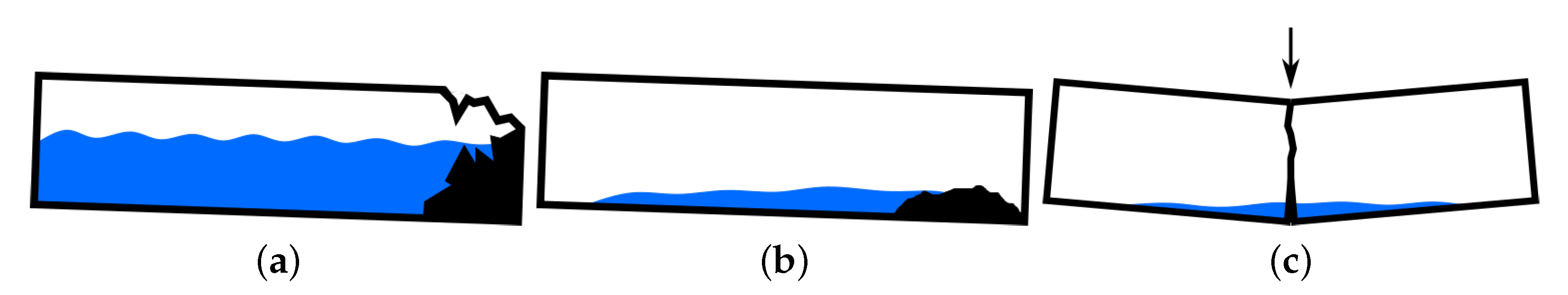
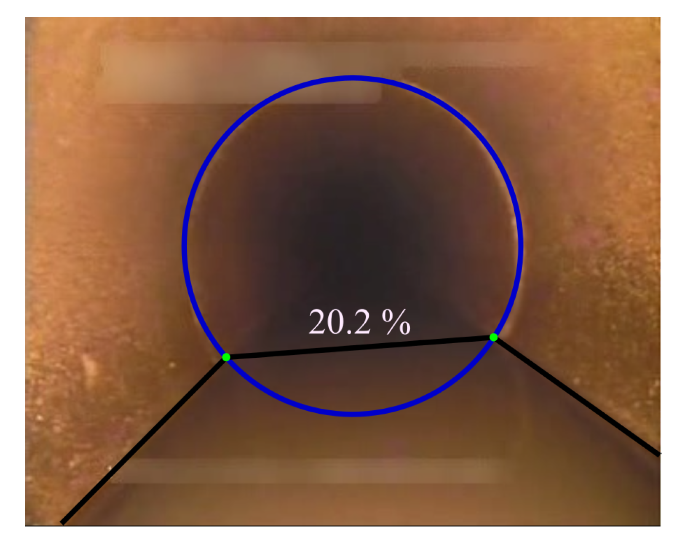
This work addresses the specific problem of water level estimation. The water level is defined as the percentage of standing water inside a sewer section. Knowing that sewer pipes are designed to follow a constant decline towards the sewer outlet, standing water should not occur unless a defect is present. High standing water could be the result of a sewer collapse (see Figure 1a). The water level is a good indicator of a sewer defect in cases where the collapse cannot be reached by the teleoperated robot. Accumulation of sediment is another cause of elevated levels of standing water (see Figure 1b). Finally, standing water can be caused by bent or broken pipes, e.g., due to ground displacement (see Figure 1c).

Considering that a video feed is the only tool that inspectors have available to make judgements, these estimates are highly inaccurate and subjective. Consequently, estimating water levels with an automatic and objective method will improve the quality control of sewers. One can think of several methods to solve this problem; classic computer vision techniques, such as extracting contours information, texture or frequency features, Scale-invariant Feature Transform (SIFT by Lowe [6]), or GIST descriptors with Gabor filters (Oliva and Torralba [7]). Afterward, the features can be sent to any appropriate classifier or regressor. Considering that Deep Learning techniques have been thoroughly proven to outperform such methods in general (Krizhevsky et al. [8]) and for sewer water level in particular (Haurum et al. [9]), we will focus our efforts on Convolutional Neural Networks (CNN).

When implementing Deep Learning techniques for industrial applications, the main consideration is the data requirements of Deep Neural Networks. As a result of the large amounts of data that are needed for the networks to learn proper representations, fully supervised learning can be a challenge. A potential solution lies in self-supervised learning, where the supervision is generated from the data itself instead of human-generated labels. Here, a learning task is designed using only the available unlabeled data. While the learning task is not necessarily directly related to the objective, it should be chosen such that solving it results in representations that are applicable to the downstream objective. While a range of methods fall under the category of self-supervised learners, we focus on Autoencoders (AEs), a type of Neural Network that learns to produce representations of data by attempting to reconstruct an input image under one or more constraints. Although AEs need a significant amount of data, the self-supervision means that the data does not have to be labeled. The representations learned by the AE may then be used for solving subsequent tasks such as classification or regression. By training AEs using a large database of sewer images, we explore semi-supervised learning, where the intention is to learn robust and general latent representations from a large unlabeled dataset before using a small labeled dataset for the regression or classification task. It will be proven that thanks to the power of the AEs as great feature extractors, less data than usual will be needed to learn water level estimation by connecting afterwards a Multi-Layer Perceptron (MLP) working as a regressor or classifier. It will also be shown how water levels in-between classes can be extracted with the MLP working as a regressor. This would simplify the process of adapting the models to different sewer inspection standards. For example, EU regulation UNE-EN 13508-2:2003 + A1:2012 [2], requires for a value as close to the reality as possible, while the 2015 version of the DANVA-Fotomanualen [3] manual splits the water levels into four different classes.

Contributions

We show how challenges with acquiring large amounts of quality data for supervised learning can be minimized by using large amounts of unlabeled data for learning meaningful latent representation using AEs. By using the latent representation together with a small amount of high-quality labeled data, it is possible to estimate a continuous output, i.e., information between classes.

The contributions can be summarized as follows:

• Demonstrate the feasibility of using large amounts of unlabeled data to improve performance in a challenging real-world computer vision application.
• Compare supervised and semi-supervised methods for water level estimation.
• Compare the performance of state-of-the-art supervised and self-supervised methods in terms of their resulting latent spaces’ ability to distinguish between different water levels.
• It is shown that AE latent space representations have enough information to extract correlative meaning from discrete classes.

2. Dataset

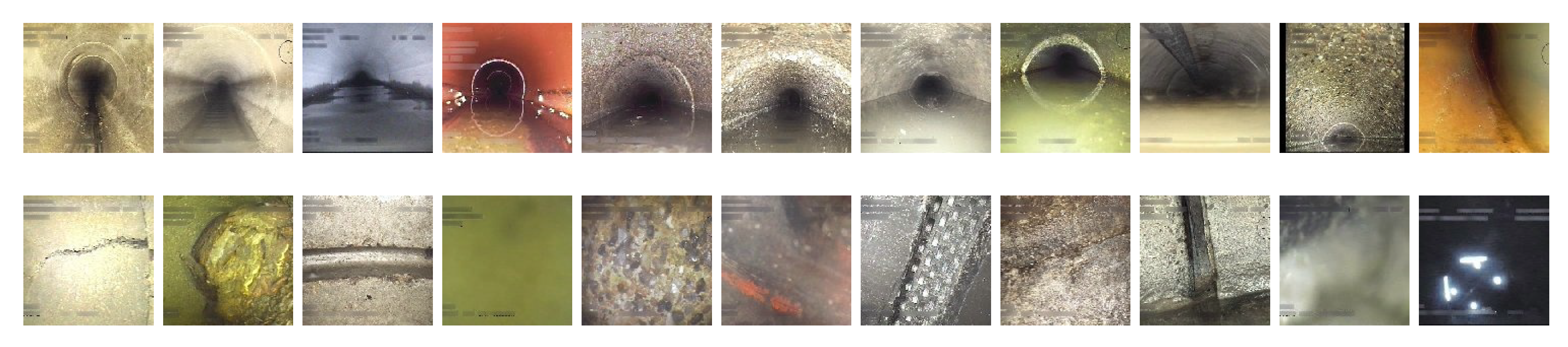
The dataset that is used in this work is called Sewer-ML. It was published by Haurum and Moeslund [10] in 2021 and consists of images from 75,618 Closed-Circuit Television (CCTV) sewer inspection videos. The videos were collected by Danish sewer inspection companies between 2011 and 2019. The dataset consists of 1,300,201 images covering 18 different classes from sewer defects and structural elements. Some samples can be seen in Figure 2.

It is worth mentioning how the database was crafted in order to understand the data being used. Each sewer inspection video comes with a report delivered by the operator. The report contains all the observations made by the operator during the inspection. The authors of Sewer-ML were able to extract interesting samples and labels from the raw videos using these reports.

However, sometimes the camera scene can be mismatched compared to the label. This is due to robot movements made by the operator around the time when the label was assigned, e.g., the robot may be facing another direction with respect to the observation when the sample is selected. The authors have attempted to deal with these problems, but some mislabeled data are expected.

After looking at the samples from Sewer-ML, it is noticed that for higher water levels from 60% to 100%, operators tend to be more subjective since robots can not usually reach sewer sections with those levels and water waves tend to cover the camera, making it harder to accurately determine the water level. Moreover, closer water levels can be easily confused; for example, a 10% water level can be confused by a 20% if the true level is in-between, where the only reference the operator has is the pipe being inspected. For that reason, a small set of data was selected to be revised. During the process, a new label was created to represent all those images that were facing the sewer wall or were too blurred or in which the water level was not observable (Figure 2 shows some examples).

From

Table 1. Dataset specifications by water level percentage. Last column indicates how classes were grouped for the MLP training.

Dataset: Water Level
Water	# Samples	Unlabeled		Labeled		Training
Level (%)		Training	Testing	Original	Revised	Class (%)
Null	-	-	-	-	1201
0	643,206	513,658	128,415	1288	1196
	643,206	513,658	128,415	1288	2397	0
10	544,979	435,046	108,761	1524	937	10
20	72,283	56,943	14,236	1153	935	20
30	22,128	16,818	4204	1085	909	30
40	7158	4839	1210	948	992	40
50	5395	3431	858	1004	986	50
60	1695	652	163	704	743
70	659	221	56	310	404
80	867	434	108	285	192
90	439	211	61	148	88
100	1392	1020	247	160	26
	5052	2538	635	1607	1453	≥60
Total	1,300,201	1,033,273	258,319	8609	8609

, it is clear that samples for higher water levels are less common, usually for levels higher than 50%. The reason for this issue comes from the inspection robot limitations; usually, when a teleoperated robot reaches high water levels, it becomes challenging for the operator to drive the robot any further or face the camera straight to the pipe. As a consequence, water may not be visible in most of the inspection. For that reason, it makes sense to merge water levels higher than 50% into a single class. In addition, if we pay attention to class Null, it represents scenes where the water level, even if present, cannot be distinguished; hence, this class is considered as 0% water level.

The Sewer-ML database is split into three main sets: unlabeled training set, unlabeled validation set and labeled set, where the ratios are 79%, 20% and 1% accordingly. We follow a different split than the split suggested by Haurum et al. [10]. This is due to an effort to achieve a better balance in terms of different water levels as well as reduce noisy labels. More detailed information about the dataset can be found in Table 1. The samples column is the complete number of samples. The unlabeled set (data considered as unlabeled yet label is available) contains the training and validation subsets used to train the AEs. Finally, both columns of the labeled set show the same samples but show the amount before and after the revision made in this work. The last column, Training class, represents the classes used in this work for training the different tested methods.

3. Related Work

There have been other attempts to automate defect detection in sewer pipes in the literature. For example, authors Halfawy and Hengmeechai [11] use Sobel derivatives in order to detect cracks or fissures in sewer pipe surfaces. In another article, Halfawy and Hengmeechai [12] use optical flow on inspection videos in order to use the operator’s behavior as a signal, bearing in mind that the operator reduces the robot’s velocity in order to pay attention to possible faults. Afterward, video segments with potential defects are processed, using techniques such as texture analysis to detect sediments or circle search to detect displaced joints. Finally, more examples using computer vision techniques can be found. Authors Halfawy and Hengmeechai [13] search Regions of Interest (ROIs) that may have root intrusions before classification using Support Vector Machines. Myrans et al. [14] use GIST descriptors and Random Forest to classify scenes with root intrusion. An interesting approach is presented by Myrans et al. [15], which is the first attempt to use different classifiers trained using GIST descriptors to detect fault samples, and then each classifier is combined to a single one using Hidden Markov Models.

There have also been attempts to classify sewer defects using CNNs. For example, authors Makantasis et al. [16] preprocess the CCTV images by computing edges using Sobel derivatives, frequencies using the Laplacian operator and texture with Gabor filters. Then each feature is used as a channel in the input to a CNN. As another example, Kumar et al. [17] trains several small binary classifiers, and each one is devoted to a single defect: roots, deposits and cracks. The most recent examples include Qian et al. [18], where CCTV images are used to train and test a combination of two networks; one detects if the image has a defect and another one classifies it. Kumar et al. [19] use the popular YOLO object detection network to detect image regions with root incursions or sedimentary deposits. All presented works have a similar handicap—the dataset they are using tends to be too small for the problem. In the case of computer vision-based approaches, the test set is too small to derive whether there is good generalization, and for the Deep Learning approaches, there are few samples for such data-hungry methods. Moreover, samples came from the same company, place or inspection video, making the dataset incomplete considering the diversity of materials, shapes, defects, structural elements present in a sewer system. To exemplify the problem, Qian et al. [18] use 42,800 images from a private dataset collected by the same experts.

Nevertheless, recent research into automatization of sewer system inspection has gained strength. For example, Haurum et al. [9] present a water level estimation Deep Learning method as well and use the same database as the one used in this work, Sewer-ML [10]. Haurum et al. [9] use classic CNN architectures such as AlexNet and ResNet to determine the water level with an F1-Score of 62.88. Given their great results, we will use their method as our baseline.

Concluding, data are a common problem in the sewer inspection automation field. With the method presented in this work, there is still the need for huge amounts of data, but with a reduced effort in the labeling process. This can be extended to any classification problem where CNNs are chosen as part of the solution and labeled data are sparse.

Representation Learning with Autoencoders

The latent space can be understood as a representation of compressed data. In the particular case of CNNs, latent representations describe image features in a reduced space. The challenge is achieving relevant representations. Meaningful latent representations have long been known to appear through the training of Deep Neural Networks, something that has been utilized in transfer learning. A good example is the study by Jason Yosinski et al. [20], where the transition from first layers general knowledge to the specialized knowledge of deeper ones is evaluated. Another example can be found in few-shot learning by Debasmit Das and CS George Lee [21], where a CNN is trained as a classifier with multiple classes and then the acquired knowledge is used as part of the proposed approach. Image comparison, e.g., perceptual loss functions, is also a good example. For example, Justin Johnson et al. [22] use a latent space from a CNN trained as a classifier, where the encoded perceptual and semantic information is used to compute a loss function.

The idea of extracting, ideally, disentangled representations originates from linear methods such as Factor Analysis (FA), Principal Components Analysis (PCA) and sparse coding. While well understood, these approaches are insufficient when confronted with complex data such as high-resolution images, where changes in pixel space may result in non-linear interactions. Luckily, Artificial Neural Networks are known for their ability to learn non-linear relationships in complex data. AEs are a specific group of Neural Networks where the input must be reconstructed under one or more constraints. The constraints typically include passing the data through an information bottleneck or corrupting and attempting to recover parts of the input. The loss and thus the learning comes from how well the output matches the original input.

The AE is a generalization of PCA, where the non-linear properties of neural networks allows the AE to learn low-dimensional representations of non-linear relationships in high-dimensional data. Both techniques work by minimizing the reconstruction error. The principal components found by PCA and the latent vectors in the bottleneck of the AE will span the same space. However, unlike the principal components, the dimensions of the latent vectors are not likely to be orthogonal and while the principal components cover progressively less of the variance, each of the dimensions of the latent space will contain approximately the same amount of variance. The AE consists of an encoder and a decoder network. Together, they must approximate an identity function where the encoder strips away static and, in practice, also high-frequency information. The decoder then attempts to recover this information. These properties of AEs have made them useful in tasks such as compression, search, outlier detection and data synthesis. A common measure for the reconstruction error is Mean Square Error (MSE). For images, this corresponds to the Euclidean distance between the input and the reconstruction in pixel space. More advanced measures may use Euclidean distance in feature space using pre-trained CNNs as feature extractors. Finally, adversarial loss from GANs can also be used as a learning signal for AEs.

The semi-supervised method used in the work is based on the idea of using AEs as self-supervised feature learners and extractors. This idea is not novel, for example, Mohammad et al. [23] use a small AE to reduce the dimensionality of a features vector, needed to predict floods using satellite data. Moreover, Cosimo et al. [24] analyze nano-materials by training an AE and then use the knowledge encoded as part of a more complex approach. Both methods use fully-connected AEs to encode information and for Cosimo et al. [24], it is only a part of the whole approach. In the presented research, the addressed problem is solved using a convolutional AE instead, which can deal with higher dimensions, and a complex refinement or extra steps are not needed to obtain proper results.

In summary, latent space extracted using an AE will preserve non-linear relationships from higher dimensional image space into a lower dimensional space, unlike methods such as PCA, FA or sparse coding. A latent space can be extracted with different deep learning methods (CNNs, GANs, AEs, among others) and different metrics can be used to measure the latent space quality. However, the research is focused on proving the potential latent space has to properly represent images and prove that it is enough to mitigate the need for high amounts of well-crafted labels. Hence, to reduce possible unwanted effects from more advanced methods, the latent space will be obtained using AEs and the Euclidean distance to measure the reconstruction error.

4. Method

Thanks to the recent availability of the Sewer-ML database, a significant amount of data are available for this study compared to other research performed in the automatic sewer inspection field. This advantage gives us the possibility of using Deep Learning techniques to extract sewer images features. This even includes self-supervised methods, allowing us to demonstrate their potential for reducing the labeling effort. The literature shows several options for learning image representations using self-supervision. These include learning by predicting rotation (Xiaohua Zhai et al. [25]), solving jigsaw puzzles (Mehdi Noroozi and Paolo Favaro [26]), discriminating instances (Zhirong Wu et al. [27]), AEs and many more. As mentioned earlier, we have decided to focus on AEs in particular due to their ease of training and use.

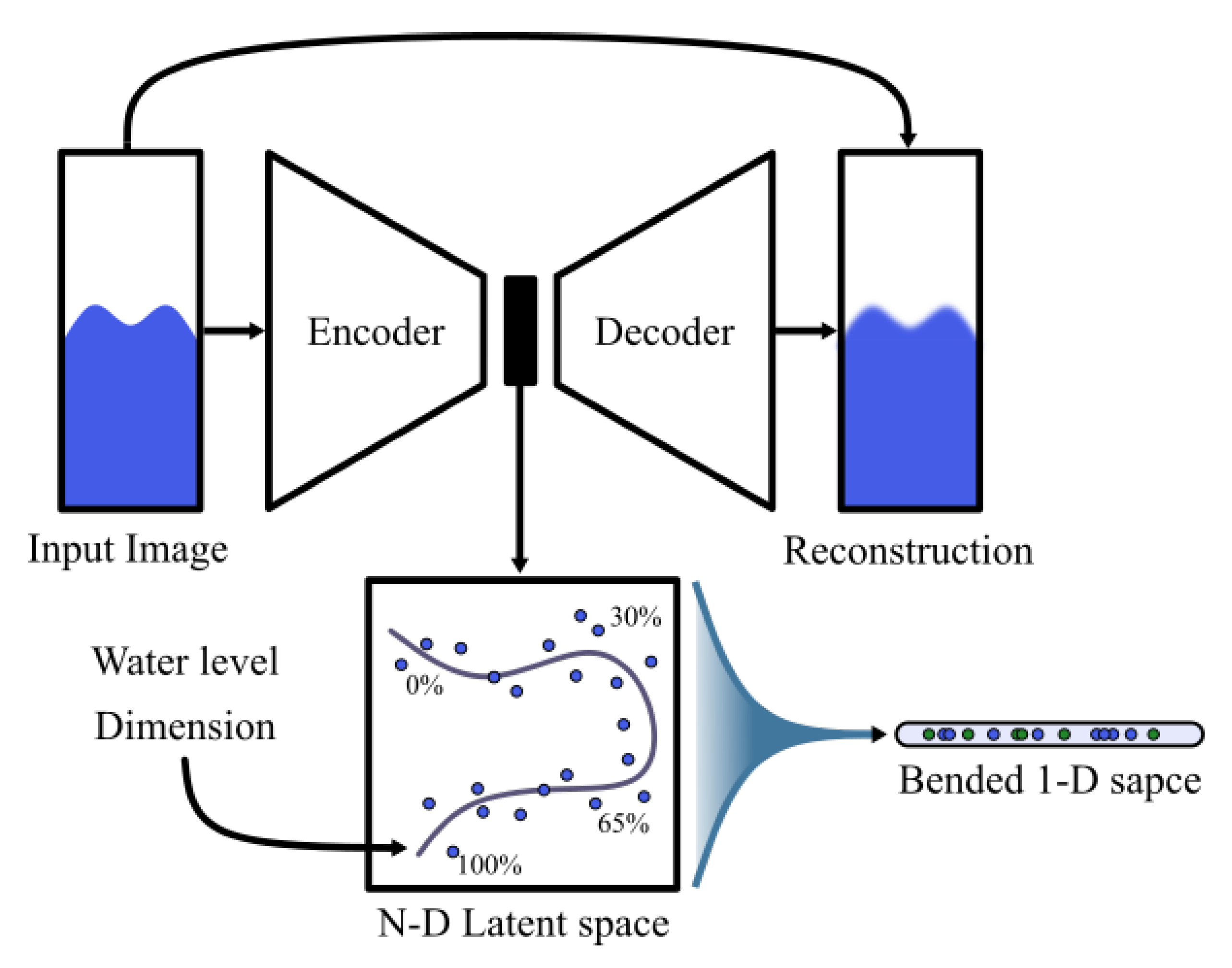
In summary, the method consists of first training an AE to learn latent representations of sewer images with unlabeled data. A small set of labeled data not seen by the AE is chosen as the training set for an MLP regressor or classifier that will learn to determine the water level. It is expected that thanks to the power of the AEs as great feature extractors, the MLP will need less data than usual to learn. Figure 3 shows the concept behind the method.

4.1. Preprocessing and Data Augmentation

The AE is trained with augmented data from the AE training dataset. The training dataset has 1,033,273 samples, where 10% of randomly selected images are augmented; hence, 103,327 new images are generated. The augmentation applied goes from image rotation, skew, noise addition, etc.

Table 2. Augmentation configuration. An image selected for an augmentation has a 50% probability of having one of the listed noises or 50% probability of being blurred (they are mutually exclusive), but the sample will have a spatial transformation.

Type	Probability	Options
Noise	50%	Gaussian Noise	Poisson Noise
		Salt and pepper	Speckle Noise
Blur	50%	Blur	Smooth
		Edge enhance	Detail
		Sharpen
Transformation	100%	Rotation	Small Zoom
		Brightness	Channel shift
		Flip	Shear

shows the augmentation strategy.

Sewer-ML is composed of CCTV RGB images of different sizes, depending on the company and/or robot that has performed the inspection. Taking into account the research purposes, it was decided to normalize the images to 128 × 128 resolution by performing a center crop and resize. The water level is still clearly visible and this resolution will help AEs to pay more attention to larger features from the image, such as the water itself. Finally, input images are normalized using a batch normalization operation to normalize the shifts between color channels. Hence, normalization will be learned during training with a batch size of 128 samples.

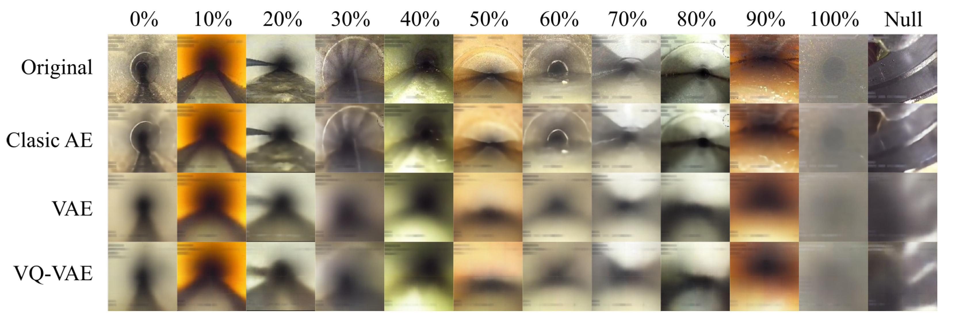
4.2. Autoencoder

Ideally one would think that once a Classic AE reaches a good reconstruction loss, taking any point from the learned latent space and using the decoder would lead to the generation a completely new and coherent image. However, over-fitting, lack of training samples, or the AE architecture can cause the loss of some relationships between data dimensions. Even though training with more than a million images, those images do not cover all the problem spectrum, and consequently, there will be encoding solutions in which latent space zones are not well defined. In other words, an AE is only trained to ensure a good reconstruction loss, but not an organized latent space without meaningless regions. For this reason, our method will also be tested using Variational Autoencoders (VAEs) since instead of encoding an image as a single representation, it encodes a distribution in the latent space. We think it is also interesting to test the presented methods using a Vector-Quantized Variational Autoencoder (VQ-VAE), which learns a discretized latent space, i.e., a finite number of latent representations, which may simplify the latent space interpretation as a feature vector.

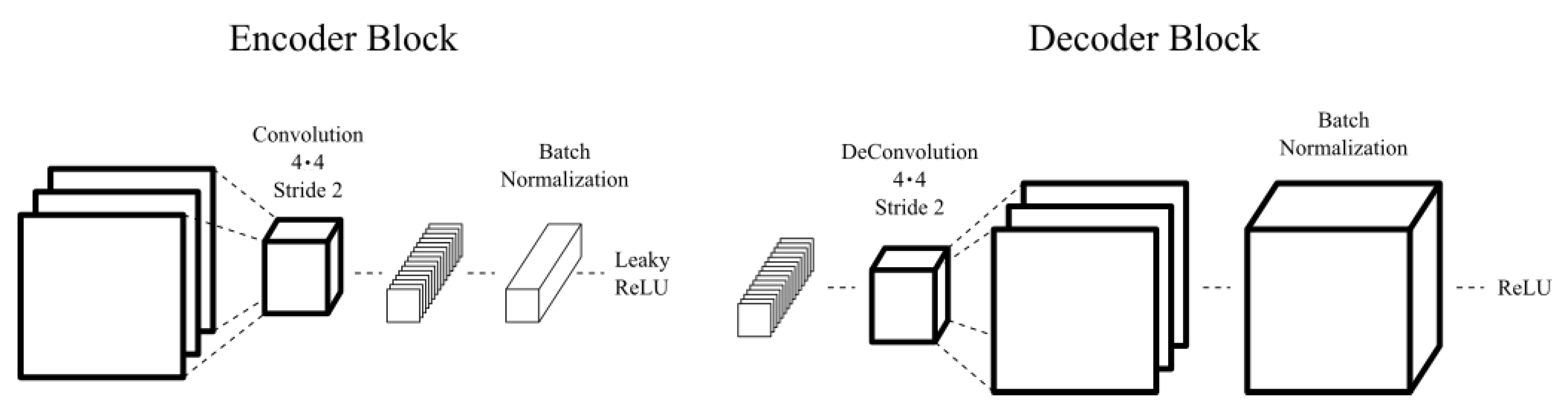
Mostly, all kinds of AEs are composed at least by an encoder and a decoder network; hence, to make the comparison fair, all AEs use the same encoder–decoder architecture. The basic convolutional module for the encoder is composed by a convolution, followed by batch normalization and a leaky-ReLU activation. Since the initial image size is 128 × 128, there will be connected six convolutional modules, with the last one being a 4 × 4 convolution without padding in order to achieve the vector representation. In addition, all reductions will be made to a 512 dimensional space, i.e., from 128 × 128 × 3 to 512.

Since we aim to have the same decoding ability as the encoder, the basic decoder deconvolutional module follows a similar architecture as the basic encoder module. First, a deconvolution with batch normalization, followed by a ReLU activation. Again, six basic modules are connected in order to go from the one dimensional representation to the 128 × 128 × 3 original image reconstruction, with the first one being a 4 × 4 deconvolution without padding and the last one having a Sigmoid activation. Figure 4 shows a sketch of the encoder and decoder basic modules with more detailed information.

All AEs that will be tested will have the same encoding and decoding capabilities. Since all of them are using the same encoder–decoder network structure, the only difference is how the latent space is constructed. For that reason, a reliable comparison between a classic AE, a VAE and a VQ-VAE is expected.

4.3. Multi-Layer Perceptron

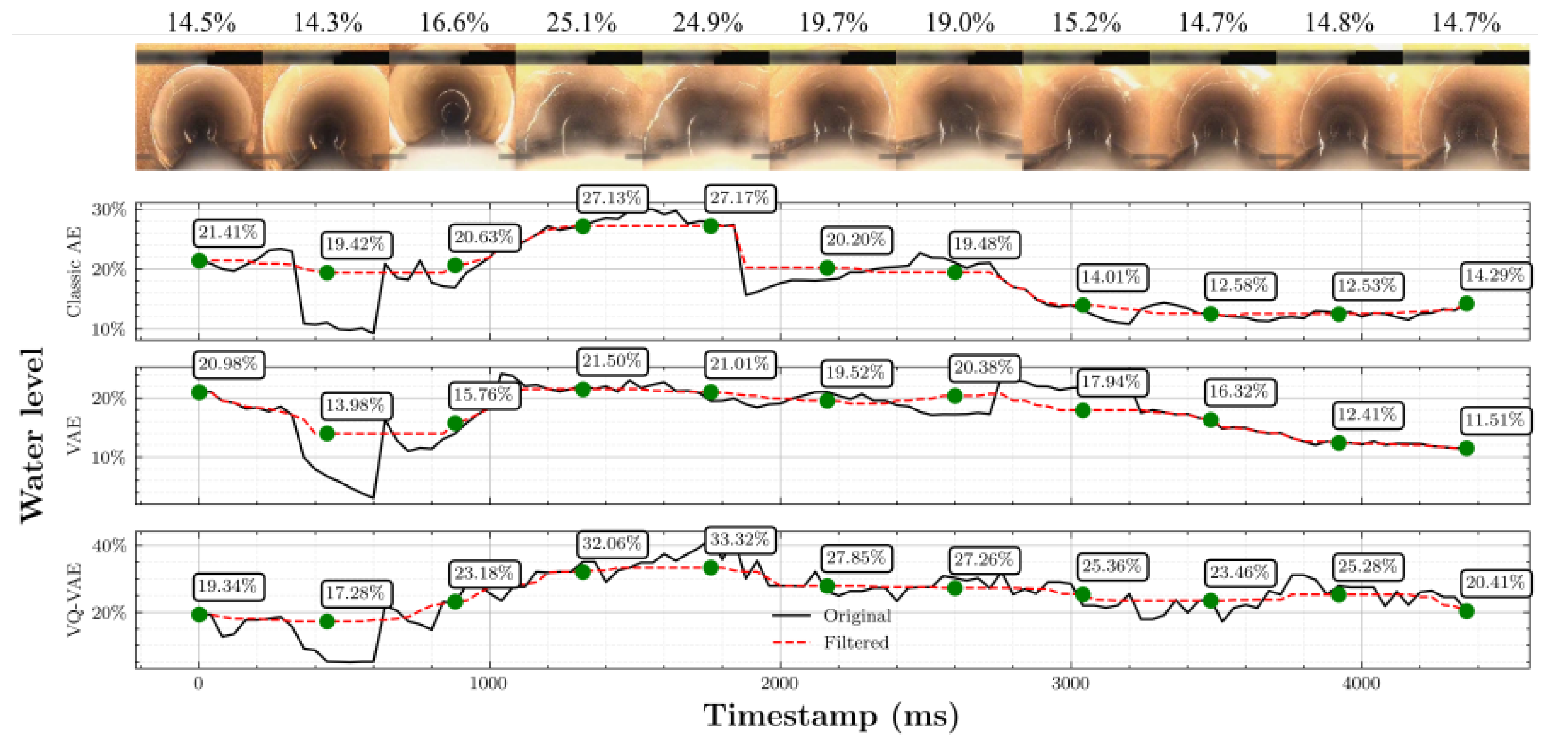
When good representations are achieved in the latent space, they can be used as a feature representation of the image, hence any classification algorithm could be used to determine the water level using the latent features produced by the encoder. Furthermore, if we pay more attention to the water level visual characteristics, differences between levels would be described by similar features. Taking a naive approach, one latent space dimension could be describing the water area, another the water texture, another the border between the water and the walls, etc. Therefore, it should be possible to use a regressor to determine the water level, making it possible to distinguish between the levels given by the dataset water level classes. On the contrary, the latent space is high dimensional where different features are not independent and they could have non-linear relationships, not to mention the possible structural information loss that might have happened during the AE training. As a consequence, a great option is to use an MLP. The MLP output will be a value from 0% to ≥60%. The Mean Squared Error (MSE) is used as the training loss. Following this strategy, we are able to identify the water level in-between two discrete classes (for example, 17% instead of 10% or 20%).

The MLP will be small since the idea is to rely on the AEs ability to efficiently represent sewer images in their latent space. We chose an MLP with a 4096-unit input layer and ReLU activation, and two hidden layers, also with 4096 units and ReLU activation. Each layer will be regularized with dropouts following Gaussian distributions and a drop rate of 10%. The output layer is a single unit with Sigmoid activation.

5. Experiments

Experiments can be split into two main groups. The first group consists of obtaining a good latent space representation and a comparison between the different models. Such tasks will be achieved by 10 trainings per AE model with the same meta-parameters configuration and data, using the unlabeled training dataset, augmented data and unlabeled validation dataset. Hence, results will be presented with the metrics mean and standard deviation to have a better comparison between methods. The training is an intermediate result, where performance will be assessed using mostly Mean Squared Reconstruction Error (MSE); see Equation (1).

$$MSE=\frac{1}{m}\sum _{i=1}^m{({\widehat{y}}_i-y_i)}^2$$

(1)

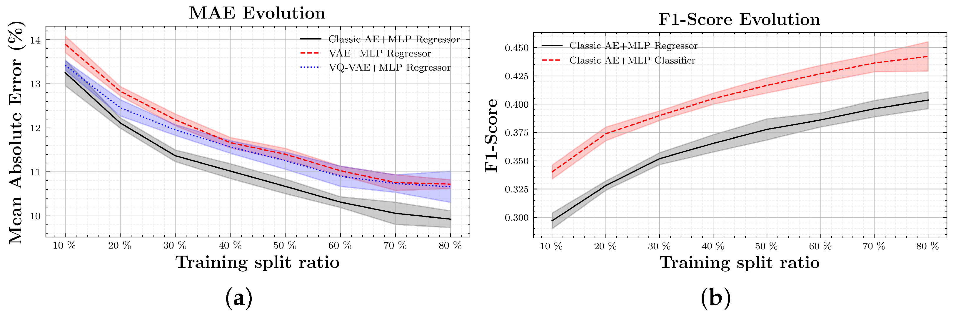
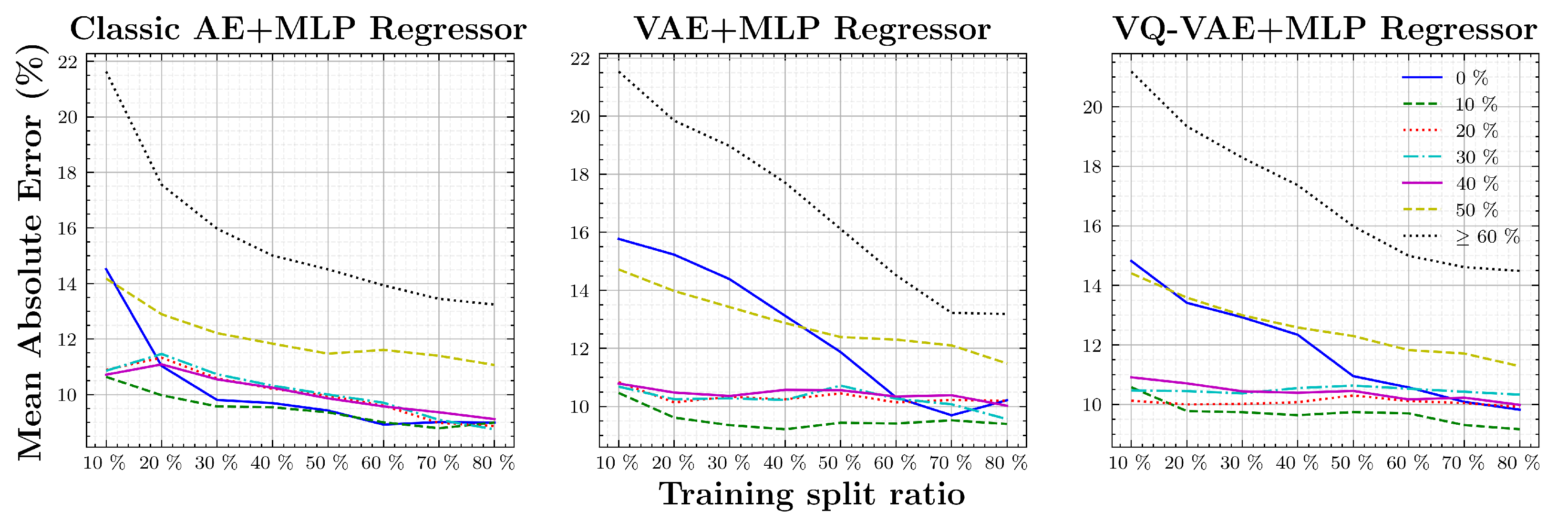
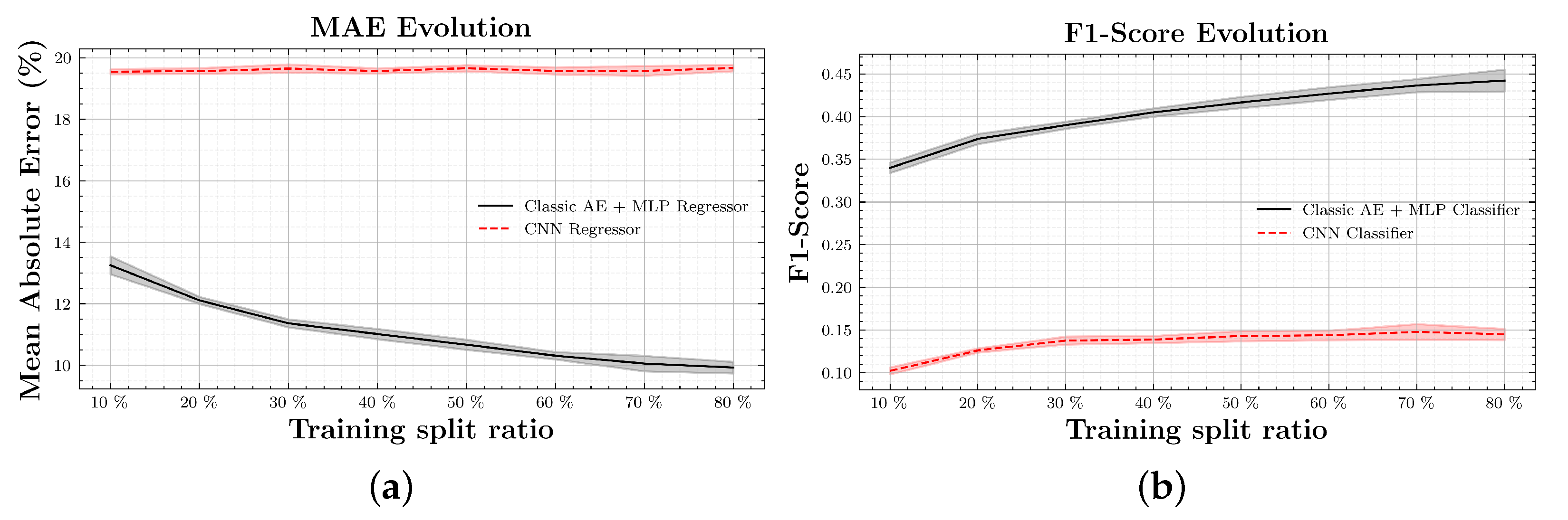
The second stage of experiments is based in the MLP training. Recalling the objective—achieve good water level classification using a small subset of labeled data—different MLP trainings with different amounts of labeled data will be performed per AE method. As explained in Section 2, the MLP dataset will be used for these experiments by splitting it into different training/validation sets ratios: 10%, 20%,…, 80%. In order to have a good baseline for comparison, from the 10 trained AEs for each model, encoders are used to compute the latent representations of the labeled dataset. Then those vectors are used to train the MLPs with eight different training splits. In the end, for a single model there are 10 AEs and 80 MLPs. Regressors will be compared using Mean Absolute Error (MAE), as defined in Equation (2), and classifiers with an F1-Score, as defined in Equation (3), where tp represents true positives, fp false positives, fn false negatives and C number of classes.

$$MAE=\frac{1}{m}\sum _{i=1}^m{\widehat{y}}_i-y_i$$

(2)

$$F_1=\frac{1}{C}\sum _{i=1}^C\frac{t{p}_i}{t{p}_i+\frac{1}{2}(f{p}_i+f{n}_i)}$$

(3)

6. Results

6.1. Autoencoder Performance

For the first set of experiments, the AE model training results can be seen in Figure 5. It can be observed that the model with the best reconstructions is the Classic AE (MSE $2.37\times {10}^{-3}$). Regarding VAE and VQ-VAE, both models obtained quite a similar reconstruction performance ($4.90\times {10}^{-3}$ and $5.03\times {10}^{-3}$ respectively); however, reconstructions made by VQ-VAE appear more detailed than the ones made by VAE (see Figure 5). It is worth mentioning how the reconstruction error for all AE models raises with increasing water levels.

6.2. Training MLP with Different Amounts of Labeled Examples

The training results of MLP regressors can be observed in Figure 6a. As expected, as more data are available for training, better results are obtained for all the AE models. Surprisingly, the best model is Classic AE, achieving an MAE of $9.93\pm 0.19$ for an 80% training split. Classic AE had the best reconstruction error; however, we expected VAE and VQ-VAE to surpass the Classic AE due to their regularization of the bottleneck. Furthermore, we can notice the difference between an MLP trained with 861 samples and the other one trained with 6888 (8 times more samples) is quite small. For the Classic AE, the improvement is only 3.33 (from 13.25 to 9.93), proving that once a good latent space is learned, the number of labeled samples needed can be dramatically reduced.

Observing Figure 7, it can be seen that the MLPs struggle more to determine higher water levels, although these are the levels that are more improved from adding more training data. By considering the labeled dataset in Table 1, it can be discarded that this difference comes from an unbalancing problem; hence, this effect can be explained by the fact that all AEs struggle more to reconstruct higher water levels samples and that the labels of such samples are more subjective than for lower water levels, also explaining why they obtain better results when more training samples are added.

In addition, an AE+MLP configured as a classifier was also trained with the different training/validation splits with the best AE method considering results from Figure 6a (Classic AE). Since, in this case, we are comparing a regressor vs. a classifier, F1-Score is used as a performance metric instead of MAE. To compute the metric for the regressor, its output will be rounded to the closest water level class. Figure 6b shows the comparison between the AE + MLP Regressor vs. the AE + MLP Classifier. The AE + MLP Classifier has an F1-Score of $0.44\pm 12.95\times {10}^{-3}$, and the AE+MLP Regressor obtains a slightly worse F1-Score, $0.40\pm 7.47\times {10}^{-3}$.

There are two main objectives in this section’s experiments: verifying water level classification can be achieved with the presented semi-supervised method, and few well-labeled samples are needed for such tasks. The labeled set (Table 1) is only around 1 % of the Sewer-ML images, but they are enough to learn the water level characteristic. Even with the 10% training split, proper results were obtained.

From Figure 6, it is demonstrated that the Classic AE + MLP Classifier has better performance than the Classic AE + MLP Regressor. This comes with the handicap of losing a continuous output that can be used to estimate water levels in-between classes. For that reason, both methods will be kept through the rest of the experiments. In doing so, it will be possible to evaluate if the drawback of choosing a regressor instead of a classifier is noteworthy.

6.3. Qualitative Results on International Sewers

INLOC Robotics SL has ceded videos with different water levels from its CCTV inspections private DataBase. Using those videos, we tested our models on real inspection data and observed how the regressor can determine a continuous water level. We have decided to show examples of pipes sections from three different inspections (Figure 8 and Figure 9). INLOC video sections do not come with water level labels, and as a consequence, to have a reference for each video sample, several equidistant frames are selected and the water level is computed following the following manual procedure. A circle is drawn following the pipe section, for example, using the joint contours as aid. Then two lines are drawn following water limits. The two intersection points from the water lines and the pipe circle conform to a new line, where the ratio between the circle area and the area below the line is the water level percentage; Figure 10 shows an example. Moreover, the water level does not change abruptly from consecutive frames in an inspection video; hence, a median filter with a window of 25 frames. This corresponds to 1 s, considering that the frame rate of the video is 25 fps.

As each sample is analyzed individually, some interesting results emerge, as we can see in the Figure 8 sequence. This sequence belongs to a slightly long video section that lasts 1 min and 15 s. The robot moves forward at slow speed, always with the camera in the pipe center. The section starts with a low water level, which increases while the robot proceeds through the pipe and decreases again at the end. This kind of behavior can be followed by any AE method, although certain peculiarities should be noted. In the case of VAE, for example, it has a smoother curve than its competitors. Since the bottleneck is regularized by a random distribution, there are minor changes in the input image (e.g., CCTV camera noise), which do not have a meaningful impact on the output. In line with this idea, similar images that go through a VQ-VAE will have exactly the same output since the latent space is discrete, consequently creating observable slopes in the graphic of the video sequence.

This effect cannot be observed at samples in Figure 9 because the sequence duration is much shorter. However, it can be observed how at the second sequence sample, the camera slightly turns towards the pipe top, making the water level less visible. As a consequence, all AE methods lower the water level estimation; however, the naive median filter is able to save the prediction.

In summary, although the real water level is not available for all the video frames, we can observe that the MLP regressor curves follow the water behavior through the inspection video interval. Therefore, water levels between classes are inferred using the latent representations.

6.4. Classic CNN Baseline

In order to make a fair comparison with the presented method against a classic supervised method, we propose to train a classic CNN assuming that the only available data are from the labeled set (Table 1). Remember that we are testing whether using this method requires fewer samples, considering that the tackled problem has a lot of data available but with few labeled samples. For that reason, in a similar situation, a supervised algorithm will only be able to use labeled samples.

With that purpose in mind, a classic CNN is trained as a regressor and a classifier using the same training splits for the labeled set (Table 1) as used to train the classic AE+MLP regressor and classifier. The network structure is composed by the encoder used in this work (Section 4.2) connected to an MLP with the same characteristics as the one described in Section 4.3. As in previous experiments, the regressors will be compared using the MAE and the classifiers of the F1-Score.

Figure 11 shows results for the CNN classifier and regressor. The proposed AE + MLP regressor significantly outperforms the classic CNN as a regressor, with the AE + MLP obtaining the best MAE $9.93\pm 0.19$ and the CNN $19.54\pm 0.09$ (Figure 11a). Taking into account the classifiers, the AE + MLP classifier also significantly outperforms the classic CNN as a classifier with the best F1-Scores $0.44\pm 12.95\times {10}^{-3}$ and $0.15\pm 9.10\times {10}^{-3}$, respectively (Figure 11b). As a conclusion, with these results it can be said that the semi-supervised method exceeds a classic supervised method when few data are available.

6.5. Summary and State-of-the-Art Comparison

Haurum et al. [9] used the Sewer-ML dataset to train several CNNs (AlexNet and ResNet) as regressors and classifiers to estimate the water level in sewer pipes. Therefore, we are able to compare our work with state-of-the-art results against the same problem. Haurum et al. [9] used the 2010 and 2015 Danish standards to train and evaluate the networks in different configurations. Since we are interested in current standards, the comparison is only performed against the 2015 norm. The standard classifies the water level in four different classes:

• water level $<5\%$
• $5\%\ge$ water level $<15\%$
• $15\%\ge$ water level $<30\%$
• $30\%\ge$ water level

Haurum et al. [9] only trained the networks as classifiers against this set of classes; hence, we decided to carry out the comparison using different configurations of our proposed solution. The original Sewer-ML datasets split was used but with an extra set to train the MLPs: 70% training set, 10% MLP training set, 10% validation set and 10% test set (training and MLP training sets belong to the original 80% training set). A classic AE is trained using the 70% training set, which is used to extract the latent space from the 10% MLP training set and train different MLP configurations.

Since classes used in this work are different from the ones used by Haurum et al. [9], we decided to train one set of MLPs using the classes from this work and then perform a comparison against the inequalities defining the four described classes. Afterward, another set of MLPs is trained using the described classes directly. In both cases, a regressor and a classifier are trained. Results can be observed in the second half of

Table 3. The first half is a summary of the results obtained in this experiment. The second half is the results of the comparison against the Haurum et al. [9] article.

Datasets	Model	MAE	F1-Score
Custom Sewer-ML datasets (Table 1)	Classic AE + MLP Reg	9.93	40.36
	Classic AE + MLP Class	-	44.23
	VAE + MLP Reg	10.72	-
	VQVAE + MLP Reg	10.66	-
	CNN Reg	19.55	-
	CNN Class	-	14.79
Original Sewer-ML datasets	Custom classes Classic AE + MLP Reg	-	49.48
	Custom classes Classic AE + MLP Class	-	50.89
	Standard classes Classic AE + MLP Reg	-	49.20
	Standard classes Classic AE + MLP Class	-	52.34
	Standard classes from scratch ResNet18 [9]	-	54.41
	Standard classes from scratch ResNet34 [9]	-	53.35
	Standard classes fine tuned ResNet50 [9]	-	62.88

.

Observing the results, it is clearly seen that Haurum et al.’s [9] best method has a better performance than the presented work. However, our method was trained using only 10% of the available labeled data, and all the AE models were trained from scratch. Therefore, it is better to compare considering Haurum et al.’s [9] models trained from scratch. In that case, the best results come from ResNet34 with an F1-Score of 53.35 and an AE+MLP classifier trained with 2015 danish standard classes with an F1-Score of 52.34, where the AE+MLP classifier still has the handicap of using fewer labeled data.

7. Conclusions

We have shown how the challenges of acquiring large amounts of quality data can be avoided by using large amounts of unlabeled data. By first training AEs using unlabeled data, their learned compressed representations can be used as features when a subsequent mapping from latent space to a target output is learned from a small amount of high-quality labeled data.

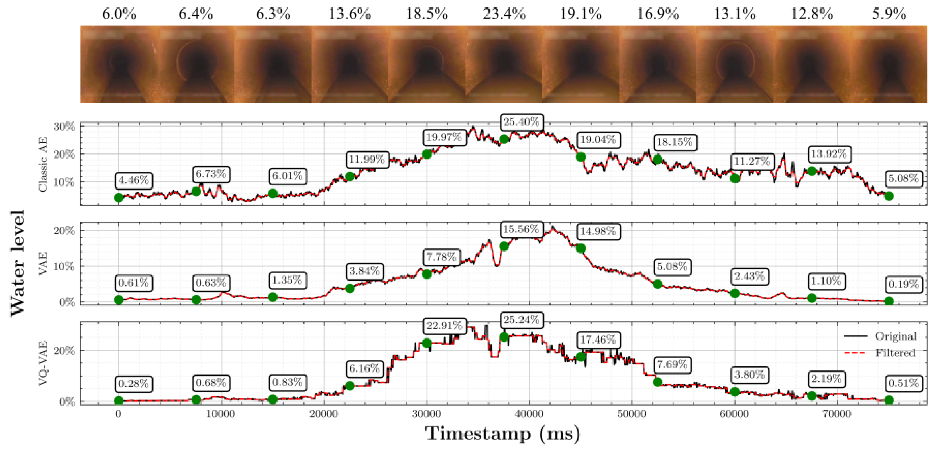
The study has shown that information that was not initially available, such as water levels between the original classes, can be extracted using the combination of AE+MLP as a regressor. This also means that this information is somehow encoded in the latent space. We have also seen that the method has better performance working as a classifier but at the expense of losing the learned information encoded in the latent space.

Results have shown that, considering a big dataset where only few data are labeled, the proposed semi-supervised AE+MLP method significantly outperforms a classic supervised CNN, assuring the complete use of the available data, labeled or unlabeled. The labeling effort is reduced dramatically.

Considering only the metrics, the best method is the classic AE combined with the MLP as a classifier followed very closely by the regressor. However, using the MLP as a classifier, we lose the ability to define the output as a continuous signal. For problems where a continuous output is relevant, such as the water level percentage modeling, it is better to drop some performance in favor of this ability.

The presented method’s performance is close to a supervised state-of-the-art work on the same dataset, yet considering the limitations (not all labeled data are used, no pre-trained weights and simple network structure), the results are very reliable, with the benefits of needing fewer labeled data.

Future Work

This work has demonstrated that the AE+MLP is able to determine continuous water levels from discrete classes, yet exact water measurements were not available in order to quantify this skill. It would be interesting to acquire well-crafted video sections with physical water level measurements in order to measure this ability.

An MLP was used as a regressor to identify the latent space dimensions that encode water level features. However, due to the MLP nature, this information is hidden in its internal structure. It might be possible to detect those dimensions using a different process where this information is not hidden. For example, Härkönen et al. [28] use PCA to identify important latent space directions in order to modify the lightning, aging, and viewpoint of a GAN-generated image. Another example is the approach of Shen and Zhou [29], where meaningful latent dimensions are found by solving a well-crafted optimization problem. Last but not least, Cohen et al. [30] achieve the exaggeration of prediction features of an arbitrary classifier using an AE and Latent Shift gradient update. Procedures such as this would open the possibility of using even fewer labeled data or none at all.

An interesting topic for further research would be the combination of different latent spaces extracted from different methods, for example, combining the latent space from the classic AE, VAE and VQ-VAE as performed by Myrans et al. [15]—in this case using different classifiers combined with Hidden Markov Models.

We have chosen the approach of training a feature extractor separate from the downstream task of water level estimation. However, alternative approaches exist, where the self-supervision and ordinary supervision are used to train the same neural network weights. This can be achieved either by fine-tuning a feature extractor for the downstream task using available labeled data or by simultaneous joint training of the self-supervision task and the labeled downstream task [25].

This approach will be extended to other target variables such as: degrees of joint displacement, blocking percent of an obstacle, amount of sedimentation, blocking percentage of a penetrating side connection, etc.