
Comparing Bayesian Model Averaging and Reliability Ensemble Averaging in Post-Processing Runoff Projections under Climate Change


Abstract
:1. Introduction
2. Methods
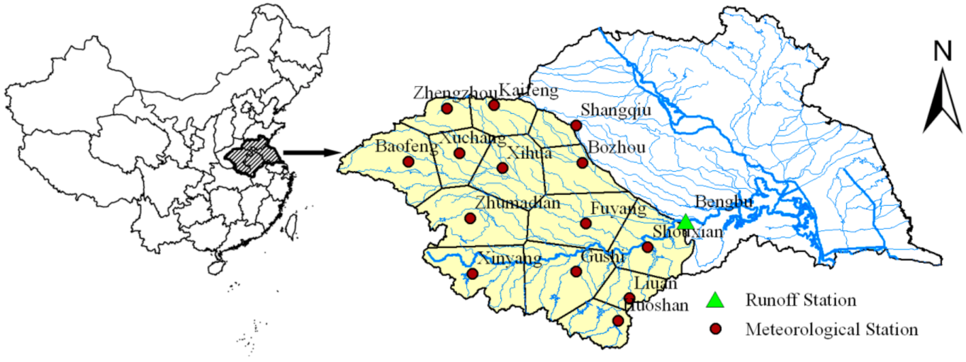
2.1. Data
2.2. Statistical Downscaling of Regional Climate
2.3. Hydrological Modeling
2.4. Probabilistic Multi-Model-Ensemble Runoff Projection
2.4.1. Bayesian Model Averaging
2.4.2. Reliability Ensemble Averaging
2.4.3. Weighting Strategies
2.5. Evaluation Metrics of Model Performance
3. Results
3.1. Model Performance in the Baseline Period
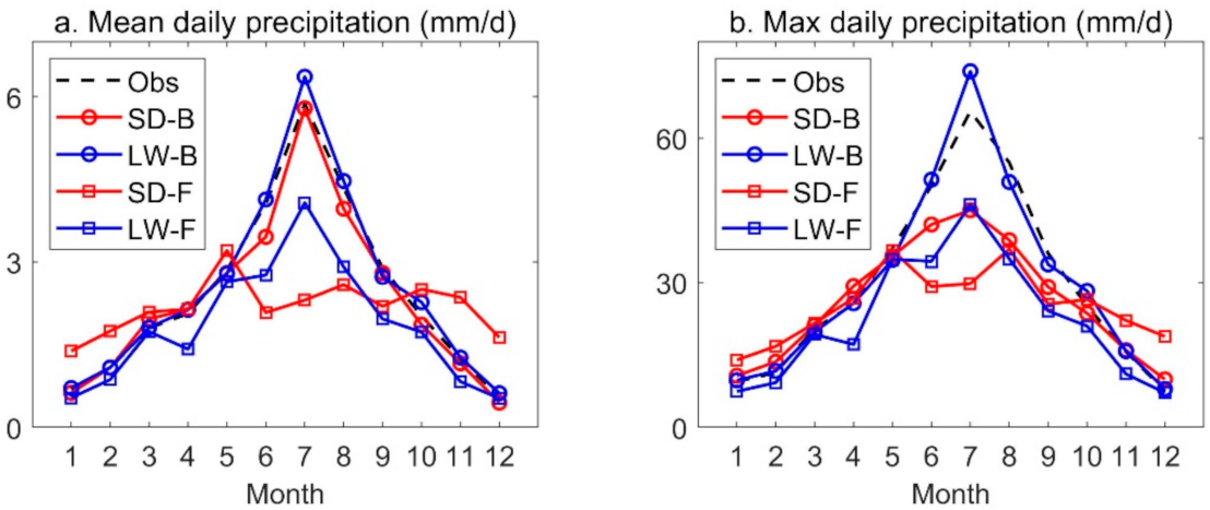
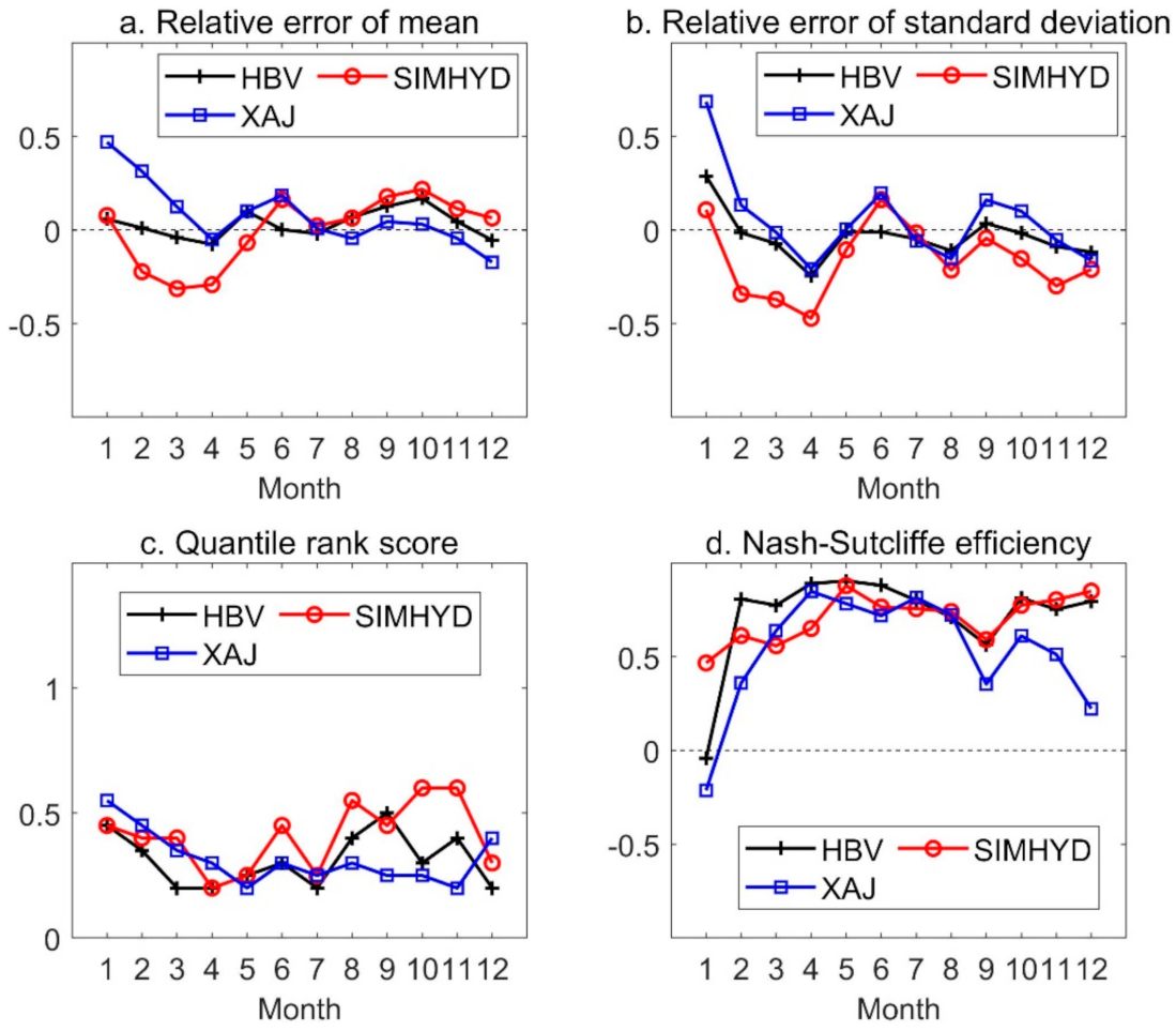
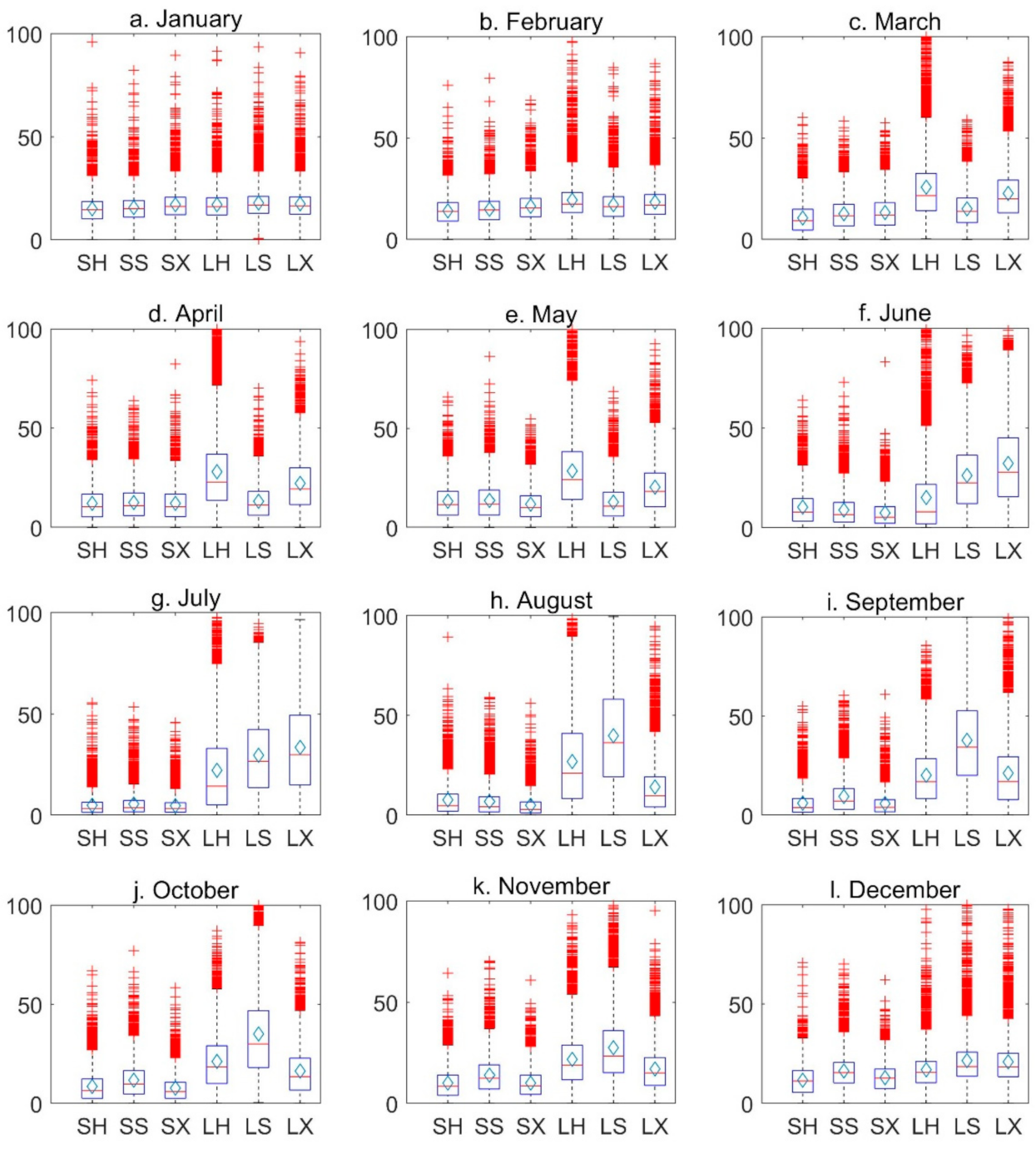
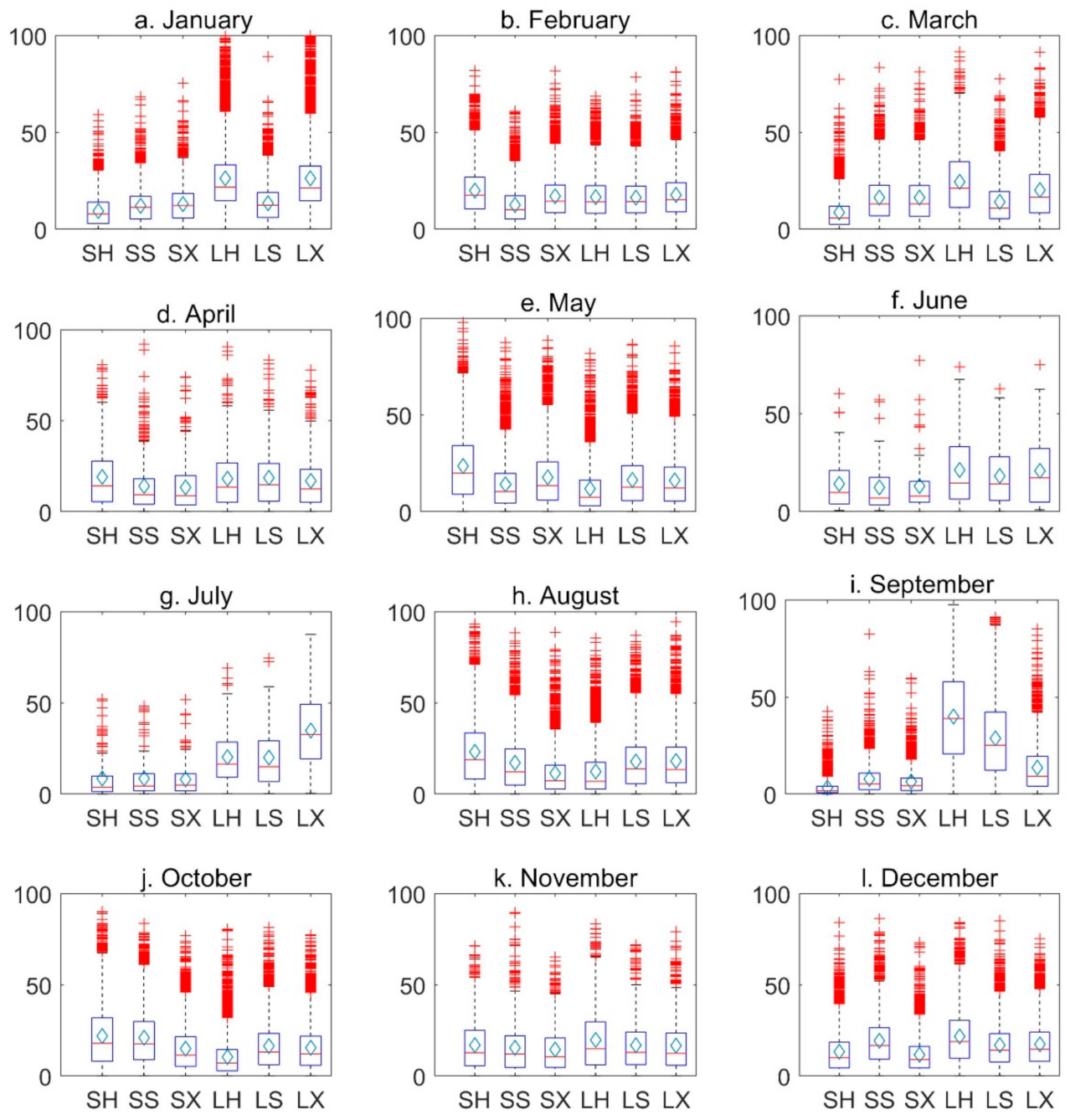
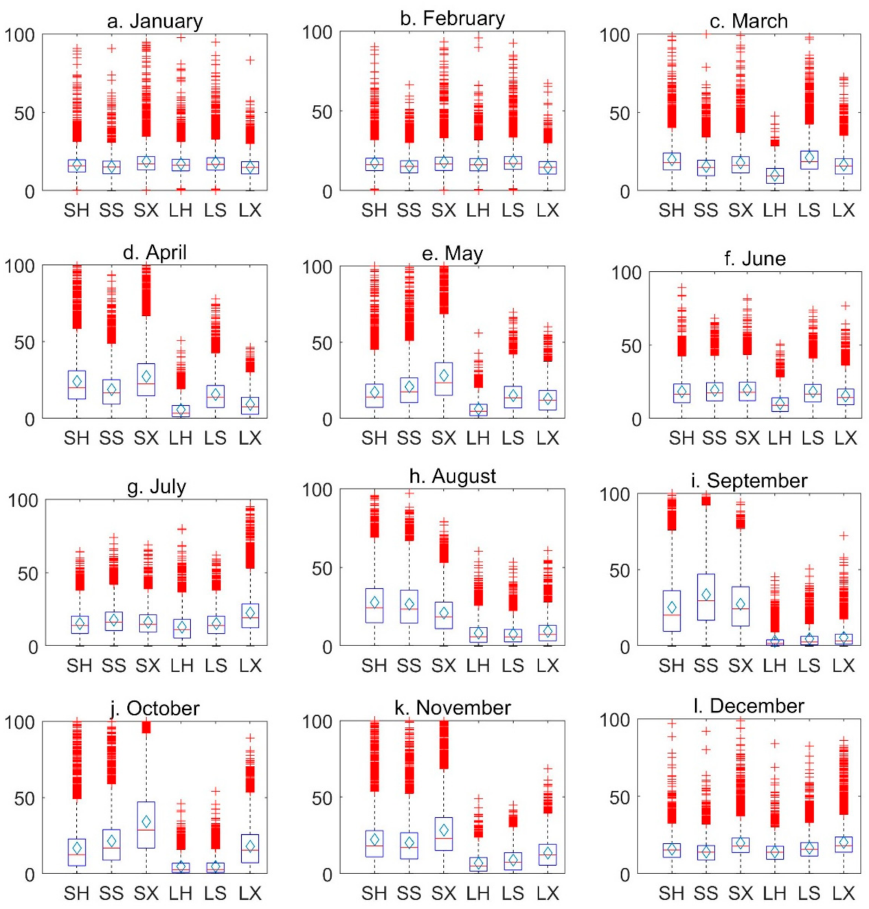
3.1.1. Individual Downscaling Models and Hydrological Models
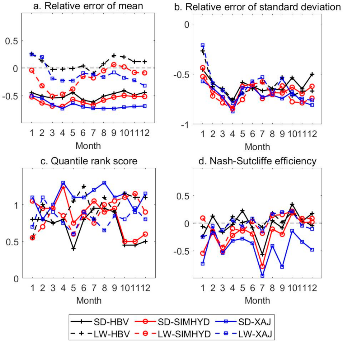
3.1.2. Combinations of Downscaling and Hydrological Models
3.2. Projected Runoff Changes in the Future
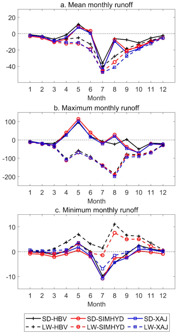
3.2.1. Projected Changes by Individual Models
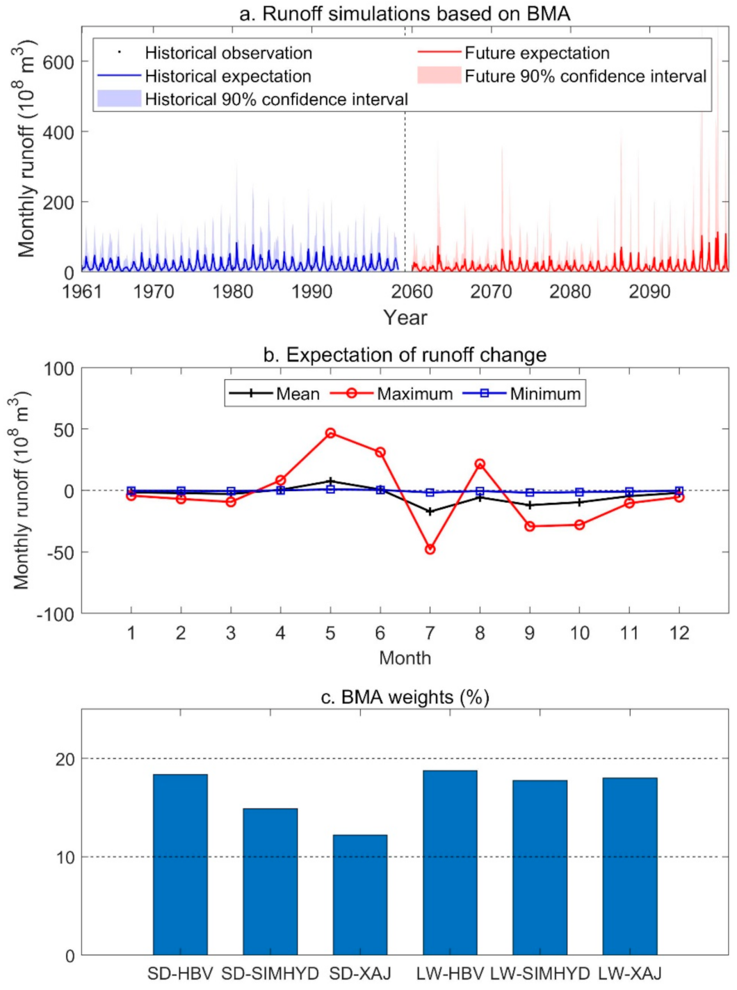
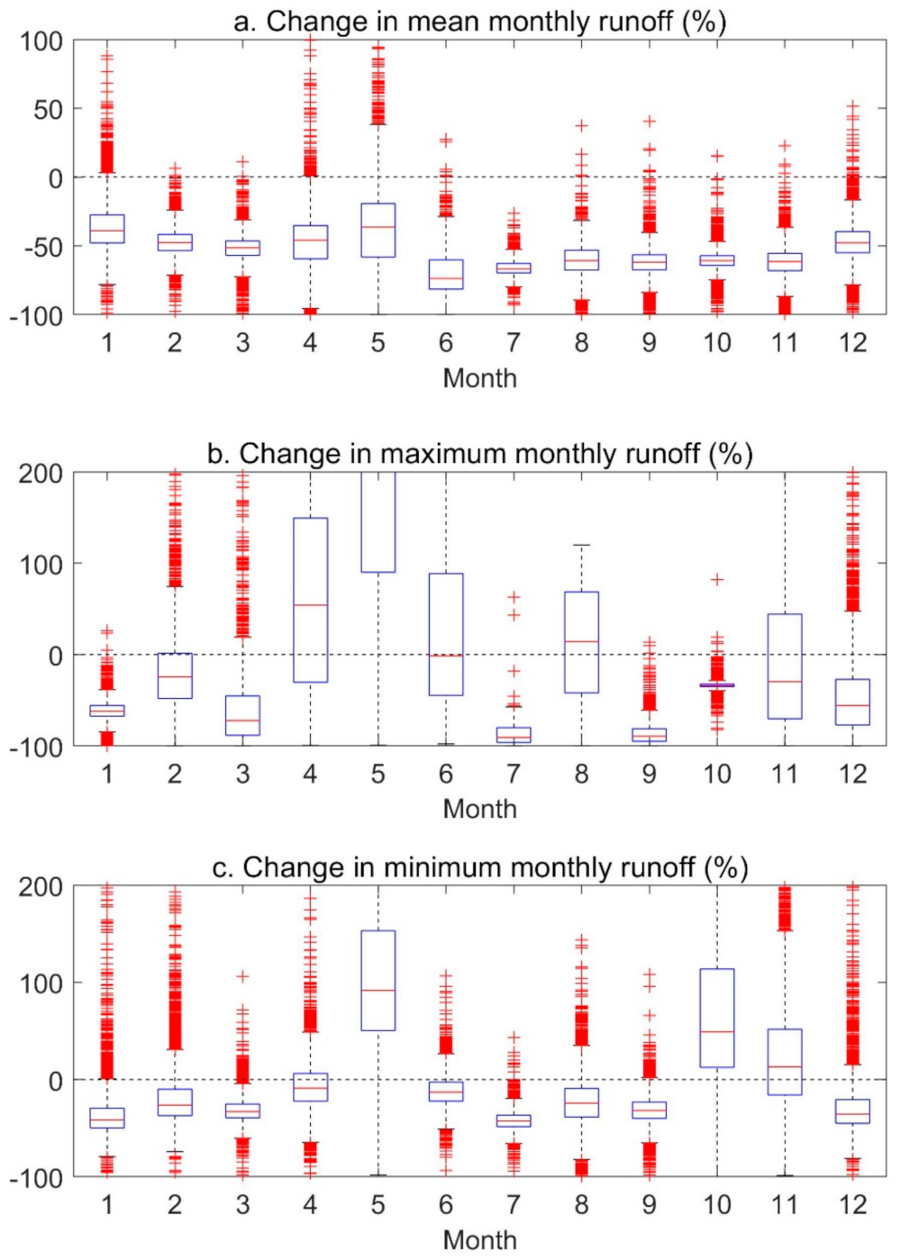
3.2.2. Posterior Distributions of Runoff Change
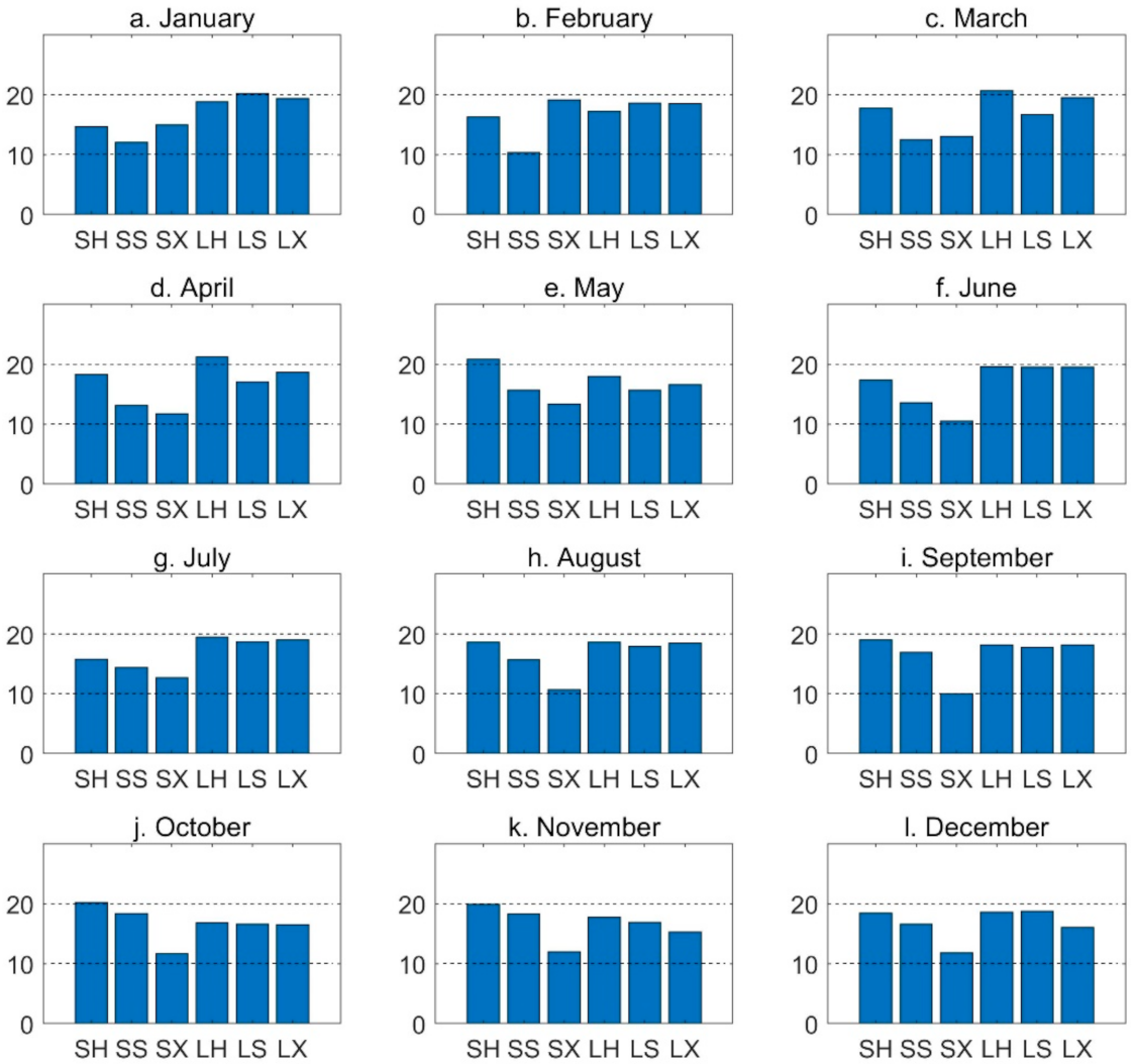
3.3. Uncertainties in Model Weighting
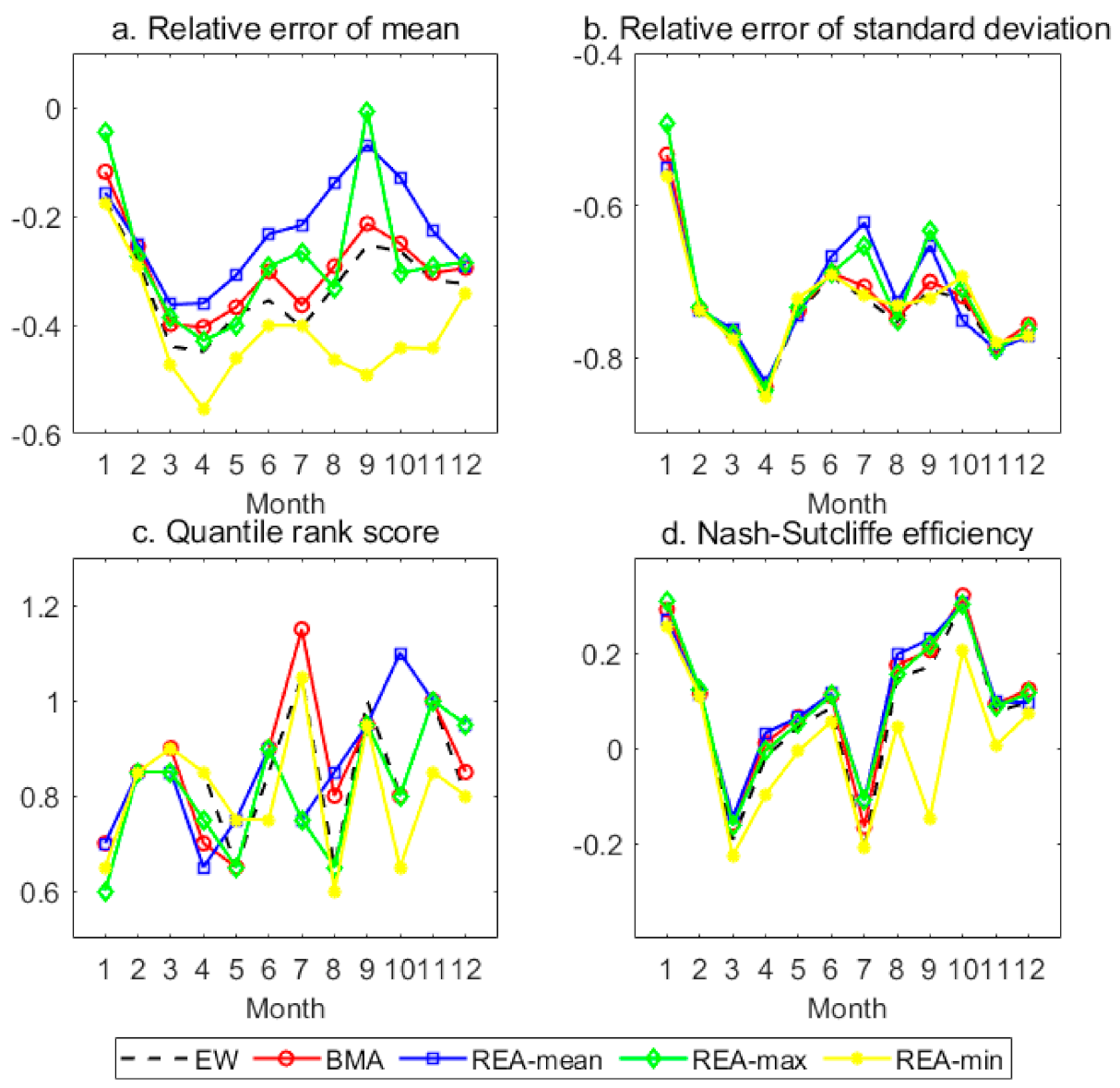
3.4. Performance of Probabilistic Multi-Model Ensembles
4. Summary and Conclusions
Author Contributions
Funding
Data Availability Statement
Conflicts of Interest
References
- Xu, C.Y. From gcms to river flow: A review of downscaling methods and hydrologic modelling approaches. Prog. Phys. Geogr. 1999, 23, 229–249. [Google Scholar] [CrossRef]
- Milly, P.C.; Dunne, K.A.; Vecchia, A.V. Global pattern of trends in streamflow and water availability in a changing climate. Nature 2005, 438, 347–350. [Google Scholar] [CrossRef] [PubMed]
- Arnell, N.W.; Gosling, S.N. The impacts of climate change on river flow regimes at the global scale. J. Hydrol. 2013, 486, 351–364. [Google Scholar] [CrossRef]
- Duan, K.; Sun, G.; McNulty, S.G.; Caldwell, P.V.; Cohen, E.C.; Sun, S.; Aldridge, H.D.; Zhou, D.; Zhang, L.; Zhang, Y. Future shift of the relative roles of precipitation and temperature in controlling annual runoff in the conterminous united states. Hydrol. Earth Syst. Sci. 2017, 21, 5517–5529. [Google Scholar] [CrossRef] [Green Version]
- Duan, K.; Caldwell, P.V.; Sun, G.; McNulty, S.G.; Zhang, Y.; Shuster, E.; Liu, B.; Bolstad, P.V. Understanding the role of regional water connectivity in mitigating climate change impacts on surface water supply stress in the united states. J. Hydrol. 2019, 570, 80–95. [Google Scholar] [CrossRef]
- Fowler, H.J.; Blenkinsop, S.; Tebaldi, C. Linking climate change modelling to impacts studies: Recent advances in downscaling techniques for hydrological modelling. Int. J. Climatol. A. J. R. Meteorol. Soc. 2007, 27, 1547–1578. [Google Scholar] [CrossRef]
- Wilby, R.L.; Charles, S.; Zorita, E.; Timbal, B.; Whetton, P.; Mearns, L. Guidelines for Use of Climate Scenarios Developed from Statistical Downscaling Methods. Supporting Material of the Intergovernmental Panel on Climate Change, Available from the DDC of IPCC TGCIA 27. 2004. Available online: https://www.ipcc-data.org/guidelines/dgm_no2_v1_09_2004.pdf (accessed on 19 July 2021).
- Chen, J.; Brissette, F.P.; Leconte, R. Uncertainty of downscaling method in quantifying the impact of climate change on hydrology. J. Hydrol. 2011, 401, 190–202. [Google Scholar] [CrossRef]
- Chiew, F.; Kirono, D.; Kent, D.; Frost, A.; Charles, S.; Timbal, B.; Nguyen, K.; Fu, G. Comparison of runoff modelled using rainfall from different downscaling methods for historical and future climates. J. Hydrol. 2010, 387, 10–23. [Google Scholar] [CrossRef]
- Duan, K.; Sun, G.; Zhang, Y.; Yahya, K.; Wang, K.; Madden, J.M.; Caldwell, P.V.; Cohen, E.C.; McNulty, S.G. Impact of air pollution induced climate change on water availability and ecosystem productivity in the conterminous united states. Clim. Chang. 2017, 140, 259–272. [Google Scholar] [CrossRef]
- Zhang, L.; Potter, N.; Hickel, K.; Zhang, Y.; Shao, Q. Water balance modeling over variable time scales based on the budyko framework—model development and testing. J. Hydrol. 2008, 360, 117–131. [Google Scholar] [CrossRef]
- Crosbie, R.S.; Scanlon, B.R.; Mpelasoka, F.S.; Reedy, R.C.; Gates, J.B.; Zhang, L. Potential climate change effects on groundwater recharge in the high plains aquifer, USA. Water Resour. Res. 2013, 49, 3936–3951. [Google Scholar] [CrossRef] [Green Version]
- Driessen, T.; Hurkmans, R.; Terink, W.; Hazenberg, P.; Torfs, P.; Uijlenhoet, R. The hydrological response of the ourthe catchment to climate change as modelled by the HBV model. Hydrol. Earth Syst. Sci. 2010, 14, 651–665. [Google Scholar] [CrossRef] [Green Version]
- Christensen, N.S.; Lettenmaier, D.P. A multimodel ensemble approach to assessment of climate change impacts on the hydrology and water resources of the colorado river basin. Hydrol. Earth Syst. Sci. 2007, 11, 1417–1434. [Google Scholar] [CrossRef] [Green Version]
- Chen, H.; Xu, C.-Y.; Guo, S. Comparison and evaluation of multiple gcms, statistical downscaling and hydrological models in the study of climate change impacts on runoff. J. Hydrol. 2012, 434, 36–45. [Google Scholar] [CrossRef]
- Dibike, Y.B.; Coulibaly, P. Hydrologic impact of climate change in the saguenay watershed: Comparison of downscaling methods and hydrologic models. J. Hydrol. 2005, 307, 145–163. [Google Scholar] [CrossRef]
- Tian, Y.; Xu, Y.-P.; Zhang, X.-J. Assessment of climate change impacts on river high flows through comparative use of gr4j, HBV and xinanjiang models. Water Resour. Manag. 2013, 27, 2871–2888. [Google Scholar] [CrossRef]
- Diks, C.G.; Vrugt, J.A. Comparison of point forecast accuracy of model averaging methods in hydrologic applications. Stoch. Environ. Res. Risk Assess. 2010, 24, 809–820. [Google Scholar] [CrossRef] [Green Version]
- Duan, K.; Mei, Y. A comparison study of three statistical downscaling methods and their model-averaging ensemble for precipitation downscaling in china. Theor. Appl. Climatol. 2014, 116, 707–719. [Google Scholar] [CrossRef]
- Duan, Q.; Ajami, N.K.; Gao, X.; Sorooshian, S. Multi-model ensemble hydrologic prediction using bayesian model averaging. Adv. Water Resour. 2007, 30, 1371–1386. [Google Scholar] [CrossRef] [Green Version]
- Wöhling, T.; Vrugt, J.A. Combining multiobjective optimization and bayesian model averaging to calibrate forecast ensembles of soil hydraulic models. Water Resour. Res. 2008, 44, 12. [Google Scholar] [CrossRef] [Green Version]
- Khan, M.S.; Coulibaly, P. Assessing hydrologic impact of climate change with uncertainty estimates: Bayesian neural network approach. J. Hydrometeorol. 2010, 11, 482–495. [Google Scholar] [CrossRef]
- Yang, T.; Hao, X.; Shao, Q.; Xu, C.-Y.; Zhao, C.; Chen, X.; Wang, W. Multi-model ensemble projections in temperature and precipitation extremes of the tibetan plateau in the 21st century. Glob. Planet. Chang. 2012, 80, 1–13. [Google Scholar] [CrossRef]
- Demirel, M.C.; Moradkhani, H.J.C.C. Assessing the impact of cmip5 climate multi-modeling on estimating the precipitation seasonality and timing. Clim. Chang. 2016, 135, 357–372. [Google Scholar] [CrossRef]
- van Vliet, M.T.; Blenkinsop, S.; Burton, A.; Harpham, C.; Broers, H.P.; Fowler, H.J. A multi-model ensemble of downscaled spatial climate change scenarios for the dommel catchment, western europe. Clim. Chang. 2012, 111, 249–277. [Google Scholar] [CrossRef] [Green Version]
- Yang, H.; Wang, B. Reducing biases in regional climate downscaling by applying bayesian model averaging on large-scale forcing. Clim. Dyn. 2012, 39, 2523–2532. [Google Scholar] [CrossRef]
- Nury, A.H.; Sharma, A.; Marshall, L.; Mehrotra, R. Characterising uncertainty in precipitation downscaling using a bayesian approach. Adv. Water Resour. 2019, 129, 189–197. [Google Scholar] [CrossRef]
- Hashmi, M.; Shamseldin, A.; Melville, B. Statistical downscaling of precipitation: State-of-the-art and application of bayesian multi-model approach for uncertainty assessment. Hydrol. Earth Syst. Sci. Discuss. 2009, 6, 6535–6579. [Google Scholar]
- Maraun, D.; Wetterhall, F.; Ireson, A.; Chandler, R.; Kendon, E.; Widmann, M.; Brienen, S.; Rust, H.; Sauter, T.; Themeßl, M. Precipitation downscaling under climate change: Recent developments to bridge the gap between dynamical models and the end user. Rev. Geophys. 2010, 48, RG3003. [Google Scholar] [CrossRef]
- Raftery, A.E.; Gneiting, T.; Balabdaoui, F.; Polakowski, M. Using bayesian model averaging to calibrate forecast ensembles. Mon. Weather Rev. 2005, 133, 1155–1174. [Google Scholar] [CrossRef] [Green Version]
- Liu, Z.; Merwade, V. Accounting for model structure, parameter and input forcing uncertainty in flood inundation modeling using bayesian model averaging. J. Hydrol. 2018, 565, 138–149. [Google Scholar] [CrossRef]
- Duan, K.; Mei, Y. Comparison of meteorological, hydrological and agricultural drought responses to climate change and uncertainty assessment. Water Resour. Manag. 2014, 28, 5039–5054. [Google Scholar] [CrossRef]
- Giorgi, F.; Mearns, L.O. Calculation of average, uncertainty range, and reliability of regional climate changes from aogcm simulations via the “reliability ensemble averaging”(rea) method. J. Clim. 2002, 15, 1141–1158. [Google Scholar] [CrossRef]
- Wilby, R.L.; Hay, L.E.; Leavesley, G.H. A comparison of downscaled and raw gcm output: Implications for climate change scenarios in the san juan river basin, colorado. J. Hydrol. 1999, 225, 67–91. [Google Scholar] [CrossRef]
- Semenov, M.A.; Stratonovitch, P. Use of multi-model ensembles from global climate models for assessment of climate change impacts. Clim. Res. 2010, 41, 1–14. [Google Scholar] [CrossRef] [Green Version]
- Seibert, J. Estimation of parameter uncertainty in the HBV model: Paper presented at the nordic hydrological conference (akureyri, iceland-august 1996). Hydrol. Res. 1997, 28, 247–262. [Google Scholar] [CrossRef]
- Seibert, J. HBV-Light, Users Manual Version 2; Department of Physical Geography, Stockholm University: Stockholm, Sweden, 2005. [Google Scholar]
- Tan, K.; Chiew, F.; Grayson, R.; Scanlon, P.; Siriwardena, L. Calibration of a Daily Rainfall-Runoff Model to Estimate High Daily Flows. In Proceedings of the MODSIM 2005 International Congress on Modelling and Simulation, Melbourne, Australia, 12–15 December 2005; pp. 2960–2966. Available online: https://citeseerx.ist.psu.edu/viewdoc/download?doi=10.1.1.375.5625&rep=rep1&type=pdf (accessed on 19 July 2021).
- Zhao, R.-J. The xinanjiang model applied in china. J. Hydrol. 1992, 135, 371–381. [Google Scholar]
- Duan, K.; Xiao, W.; Mei, Y.; Liu, D. Multi-scale analysis of meteorological drought risks based on a bayesian interpolation approach in huai river basin, china. Stoch. Environ. Res. Risk Assess. 2014, 28, 1985–1998. [Google Scholar] [CrossRef]
- Kalnay, E.; Kanamitsu, M.; Kistler, R.; Collins, W.; Deaven, D.; Gandin, L.; Iredell, M.; Saha, S.; White, G.; Woollen, J. The ncep/ncar 40-year reanalysis project. Bull. Am. Meteorol. Soc. 1996, 77, 437–472. [Google Scholar] [CrossRef] [Green Version]
- Duan, K.; Mei, Y. Uncertainty analysis of precipitation change based on tebaldi multimodel ensemble method. Eng. J. Wuhan Univ. 2015, 048, 433–440. [Google Scholar]
- Tebaldi, C.; Mearns, L.O.; Nychka, D.; Smith, R.L. Regional probabilities of precipitation change: A bayesian analysis of multimodel simulations. Geophys. Res. Lett. 2004, 31, L24213. [Google Scholar] [CrossRef] [Green Version]
- Tebaldi, C.; Smith, R.L.; Nychka, D.; Mearns, L.O. Quantifying uncertainty in projections of regional climate change: A bayesian approach to the analysis of multimodel ensembles. J. Clim. 2005, 18, 1524–1540. [Google Scholar] [CrossRef] [Green Version]
- Lopez, A.; Tebaldi, C.; New, M.; Stainforth, D.; Allen, M.; Kettleborough, J. Two approaches to quantifying uncertainty in global temperature changes. J. Clim. 2006, 19, 4785–4796. [Google Scholar] [CrossRef]
- Hashmi, M.Z.; Shamseldin, A.Y.; Melville, B.W. Statistically downscaled probabilistic multi-model ensemble projections of precipitation change in a watershed. Hydrol. Process. 2013, 27, 1021–1032. [Google Scholar] [CrossRef]
- Meehl, G.A.; Boer, G.J.; Covey, C.; Latif, M.; Stouffer, R.J. The coupled model intercomparison project (cmip). Bull. Am. Meteorol. Soc. 2000, 81, 313–318. [Google Scholar] [CrossRef] [Green Version]
- Georgakakos, K.P.; Seo, D.-J.; Gupta, H.; Schaake, J.; Butts, M.B. Towards the characterization of streamflow simulation uncertainty through multimodel ensembles. J. Hydrol. 2004, 298, 222–241. [Google Scholar] [CrossRef]
- Yu, G.; Fu, Y.; Sun, X.; Wen, X.; Zhang, L. Recent progress and future directions of chinaflux. Sci. China Ser. D Earth Sci. 2006, 49, 1–23. [Google Scholar] [CrossRef]
- Smith, R.L.; Tebaldi, C.; Nychka, D.; Mearns, L.O. Bayesian modeling of uncertainty in ensembles of climate models. J. Am. Stat. Assoc. 2009, 104, 97–116. [Google Scholar] [CrossRef]
- Pachauri, R.K.; Allen, M.R.; Barros, V.R.; Broome, J.; Cramer, W.; Christ, R.; Church, J.A.; Clarke, L.; Dahe, Q.; Dasgupta, P.; et al. Climate Change 2014: Synthesis Report. Contribution of Working Groups I, II and III to the Fifth Assessment Report of the Intergovernmental Panel on Climate Change; IPCC: Geneva, Switzerland, 2014; ISBN 9291691437. [Google Scholar]
- Giuntoli, I.; Vidal, J.-P.; Prudhomme, C.; Hannah, D.M. Future hydrological extremes: The uncertainty from multiple global climate and global hydrological models. Earth Syst. Dyn. 2015, 6, 267–285. [Google Scholar] [CrossRef] [Green Version]
- Knutti, R.; Sedláček, J. Robustness and uncertainties in the new cmip5 climate model projections. Nat. Clim. Chang. 2013, 3, 369–373. [Google Scholar] [CrossRef]


| Procedure | Model | Features |
|---|---|---|
| Climate downscaling | SDSM [34] | Data required—Historical precipitation, temperature, and large-scale predictors Model structure—Precipitation occurrence and magnitude fitted by multiple regressions |
| LARS-WG [35] | Data required—Historical precipitation and temperature Model structure—Precipitation occurrence and magnitude fitted by semi-empirical distributions; extreme events represented by specifying precipitation intervals | |
| Hydrological modeling | HBV [36] | Water storage components—Upper and lower groundwater storage Runoff generation regime—Saturation excess Runoff components—Peak, intermediate, and baseflow |
| SIMHYD [38] | Water storage components—Soil moisture storage and groundwater storage Runoff generation regime—Saturation excess and infiltration excess Runoff components—Infiltration excess runoff, interflow, and baseflow | |
| XAJ [39] | Water storage components—Upper, lower, and deep tension water storage, free water storage Runoff generation regime—Saturation excess Runoff components—surface runoff, interflow, groundwater flow | |
| Model ensemble | BMA [20,30] | Uncertainty interpretation—Bayesian probability Weighting criteria—Models’ relative contributions to predictive skill Parameter estimation—Expectation maximization algorithm |
| REA [33,43] | Uncertainty interpretation—Bayesian probability Weighting criteria—Model bias and model convergence Parameter estimation—Gibbs-Metropolis algorithm |
Publisher’s Note: MDPI stays neutral with regard to jurisdictional claims in published maps and institutional affiliations. |
© 2021 by the authors. Licensee MDPI, Basel, Switzerland. This article is an open access article distributed under the terms and conditions of the Creative Commons Attribution (CC BY) license (https://creativecommons.org/licenses/by/4.0/).
Share and Cite
Duan, K.; Wang, X.; Liu, B.; Zhao, T.; Chen, X. Comparing Bayesian Model Averaging and Reliability Ensemble Averaging in Post-Processing Runoff Projections under Climate Change. Water 2021, 13, 2124. https://doi.org/10.3390/w13152124
Duan K, Wang X, Liu B, Zhao T, Chen X. Comparing Bayesian Model Averaging and Reliability Ensemble Averaging in Post-Processing Runoff Projections under Climate Change. Water. 2021; 13(15):2124. https://doi.org/10.3390/w13152124
Chicago/Turabian StyleDuan, Kai, Xiaola Wang, Bingjun Liu, Tongtiegang Zhao, and Xiaohong Chen. 2021. "Comparing Bayesian Model Averaging and Reliability Ensemble Averaging in Post-Processing Runoff Projections under Climate Change" Water 13, no. 15: 2124. https://doi.org/10.3390/w13152124