Are Biocrusts and Xerophytic Vegetation a Viable Green Roof Typology in a Mediterranean Climate? A Comparison between Differently Vegetated Green Roofs in Water Runoff and Water Quality

 ,
,  ,
,  , ,
, ,  ,
,
Abstract
:1. Introduction
2. Materials and Methods
2.1. Study Area
2.2. Vegetation Composition, Functional Traits and Cover
2.3. Methodologies Used to Assess Ecosystem Services
2.3.1. Stormwater Management
2.3.2. Runoff Quality
2.4. Statistical Analysis
3. Results
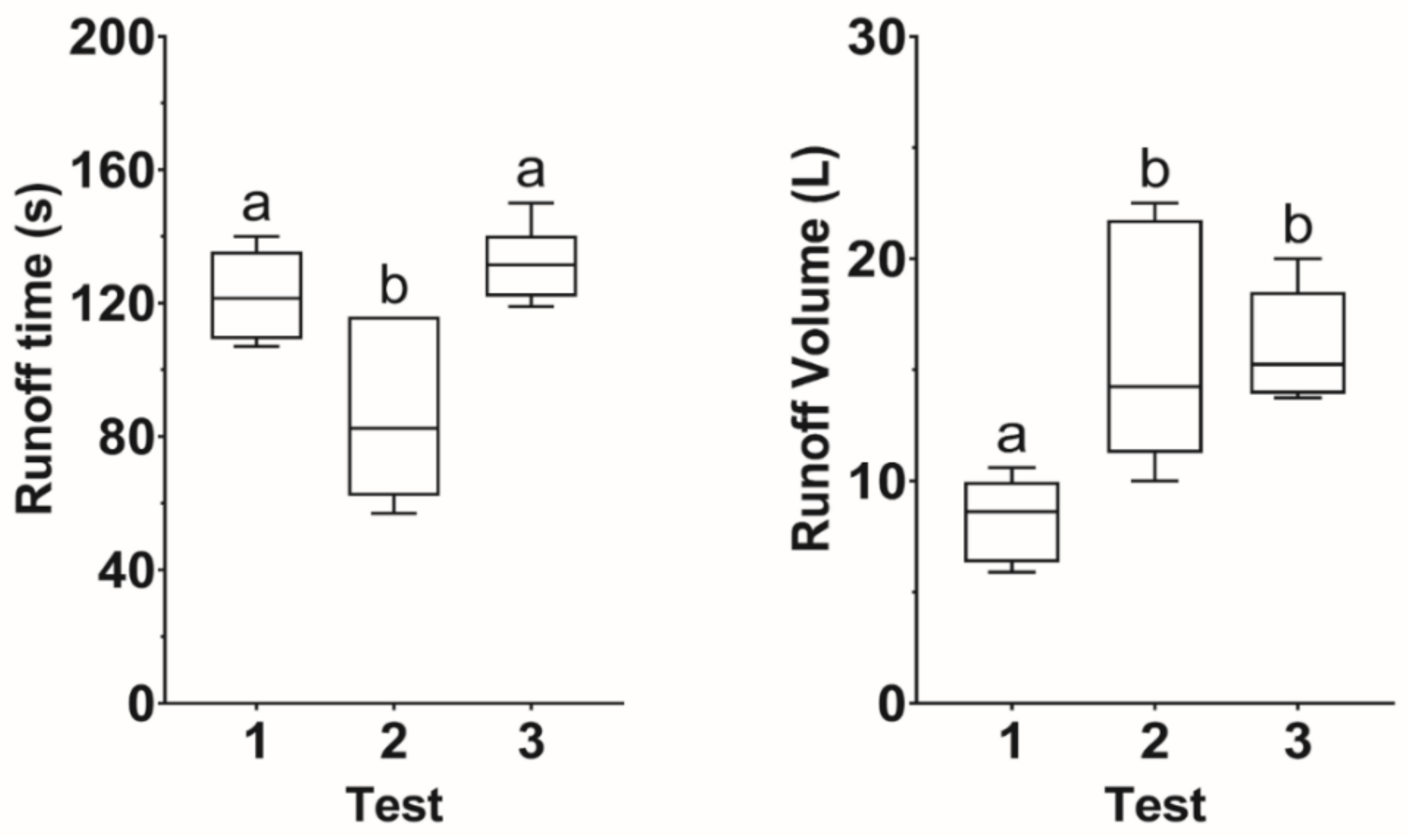
3.1. Stormwater Management
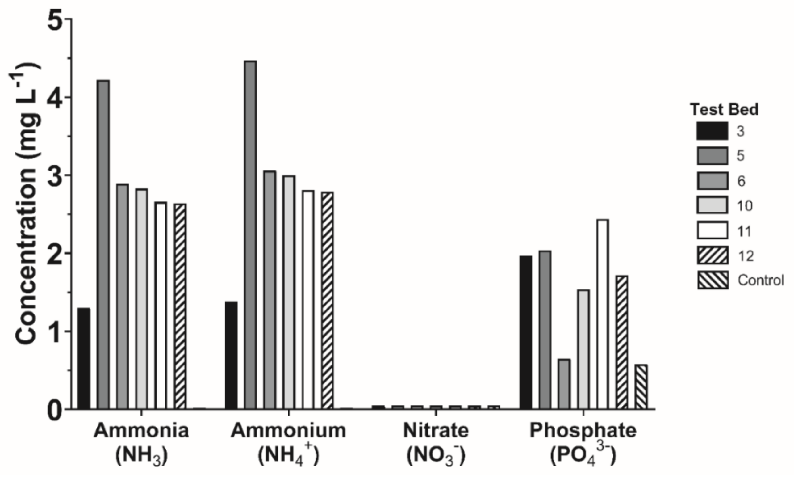
3.2. Runoff Quality
4. Discussion
5. Conclusions
Supplementary Materials
Author Contributions
Funding
Institutional Review Board Statement
Informed Consent Statement
Acknowledgments
Conflicts of Interest
References
- Boyd, B. Urbanization and the Mass Movement of People to Cities; Grayline Group: Austin, TA, USA, 2018; p. 14. [Google Scholar]
- Mohajerani, A.; Bakaric, J.; Jeffrey-Bailey, T. The urban heat island effect, its causes, and mitigation, with reference to the thermal properties of asphalt concrete. J. Environ. Manag. 2017, 197, 522–538. [Google Scholar] [CrossRef] [PubMed]
- Depietri, Y.; Renaud, F.G.; Kallis, G. Heat waves and floods in urban areas: A policy-oriented review of ecosystem services. Sustain. Sci. 2011, 7, 95–107. [Google Scholar] [CrossRef]
- Houston, D.; Werritty, A.; Bassett, D.; Geddes, A.; Hoolachan, A.; McMillan, M. Pluvial (Rain-Related) Flooding in Urban Areas: The Invisible Hazard; Joseph Rowntree Foundation: York, UK, 2011. [Google Scholar]
- Guzzetti, F.; Stark, C.P.; Salvati, P. Evaluation of flood and landslide risk to the population of Italy. Environ. Manag. 2005, 36, 15–36. [Google Scholar] [CrossRef]
- Llasat, M.C.; Llasat-Botija, M.; Prat, M.A.; Porcú, F.; Price, C.; Mugnai, A.; Lagouvardos, K.; Kotroni, V.; Katsanos, D.; Michaelides, S.; et al. High-impact floods and flash floods in Mediterranean countries: The FLASH preliminary database. Adv. Geosci. 2010, 23, 47–55. [Google Scholar] [CrossRef] [Green Version]
- Gaumé, E.; Bain, V.; Bernardara, P.; Newinger, O.; Barbuc, M.; Bateman, A.; Blbakovi ová, L.; Blöschl, G.; Borga, M.; Dumitrescu, A.; et al. A compilation of data on European flash floods. J. Hydrol. 2009, 367, 70–78. [Google Scholar] [CrossRef] [Green Version]
- Amponsah, W.; Ayral, P.-A.; Boudevillain, B.; Bouvier, C.; Braud, I.; Brunet, P.; Delrieu, G.; Didon-Lescot, J.-F.; Gaume, E.; Lebouc, L.; et al. Integrated high-resolution dataset of high-intensity European and Mediterranean flash floods. Earth Syst. Sci. Data 2018, 10, 1783–1794. [Google Scholar] [CrossRef] [Green Version]
- Llasat, M.C.; Marcos, R.; Llasat-Botija, M.; Gilabert, J.; Turco, M.; Quintana-Seguí, P. Flash flood evolution in North-Western Mediterranean. Atmos. Res. 2014, 149, 230–243. [Google Scholar] [CrossRef] [Green Version]
- Ferro, G. Assessment of major and minor events that occurred in Italy during the last century using a disaster severity scale score. Prehospital Disaster Med. 2005, 20, 316–323. [Google Scholar] [CrossRef]
- Lane, K.; Charles-Guzman, K.; Wheeler, K.; Abid, Z.; Graber, N.; Matte, T. Health effects of coastal storms and flooding in urban areas: A review and vulnerability assessment. J. Environ. Public Health 2013, 2013, 913064. [Google Scholar] [CrossRef]
- Lastoria, B.; Simonetti, M.R.; Casaioli, M.; Mariani, S.; Monacelli, G. Socio-economic impacts of major floods in Italy from 1951 to 2003. Adv. Geosci. 2006, 7, 223–229. [Google Scholar] [CrossRef] [Green Version]
- McGinnigle, J.B. The 1952 Lynmouth floods revisited. Weather 2002, 57, 235–242. [Google Scholar] [CrossRef]
- Gaume, E.; Livet, M.; Desbordes, M.; Villeneuve, J.-P. Hydrological analysis of the river Aude, France, flash flood on 12 and 13 November 1999. J. Hydrol. 2004, 286, 135–154. [Google Scholar] [CrossRef]
- Fahrig, L. Effects of habitat fragmentation on biodiversity. Annu. Rev. Ecol. Evol. Syst. 2003, 34, 487–515. [Google Scholar] [CrossRef] [Green Version]
- Collingham, Y.C.; Huntley, B. Impacts of habitat fragmentation and patch size upon migration rates. Ecol. Appl. 2000, 10, 131–144. [Google Scholar] [CrossRef]
- Haddad, N.M.; Brudvig, L.A.; Clobert, J.; Davies, K.F.; Gonzalez, A.; Holt, R.D.; Lovejoy, T.E.; Sexton, J.O.; Austin, M.P.; Collins, C.D.; et al. Habitat fragmentation and its lasting impact on Earth’s ecosystems. Sci. Adv. 2015, 1, e1500052. [Google Scholar] [CrossRef] [Green Version]
- Krauss, J.; Bommarco, R.; Guardiola, M.; Heikkinen, R.K.; Helm, A.; Kuussaari, M.; Lindborg, R.; Öckinger, E.; Pärtel, M.; Pino, J.; et al. Habitat fragmentation causes immediate and time-delayed biodiversity loss at different trophic levels. Ecol. Lett. 2010, 13, 597–605. [Google Scholar] [CrossRef] [Green Version]
- Hao, J.; He, D.; Wu, Y.; Fu, L.; He, K. A study of the emission and concentration distribution of vehicular pollutants in the urban area of Beijing. Atmos. Environ. 2000, 34, 453–465. [Google Scholar] [CrossRef]
- Romero, H.; Ihl, M.; Rivera, A.; Zalazar, P.; Azocar, P. Rapid urban growth, land-use changes and air pollution in Santiago, Chile. Atmos. Environ. 1999, 33, 4039–4047. [Google Scholar] [CrossRef]
- Grosjean, D.; Miguel, A.H.; Tavares, T.M. Urban air pollution in Brazil: Acetaldehyde and other carbonyls. Atmos. Environ. Part B Urban Atmos. 1990, 24, 101–106. [Google Scholar] [CrossRef]
- Gkatsopoulos, P. A Methodology for calculating cooling from vegetation evapotranspiration for use in urban space microclimate simulations. Procedia Environ. Sci. 2017, 38, 477–484. [Google Scholar] [CrossRef]
- Oliveira, S.; Andrade, H.; Vaz, T. The cooling effect of green spaces as a contribution to the mitigation of urban heat: A case study in Lisbon. Build. Environ. 2011, 46, 2186–2194. [Google Scholar] [CrossRef]
- Ng, E.; Chen, L.; Wang, Y.; Yuan, C. A study on the cooling effects of greening in a high-density city: An experience from Hong Kong. Build. Environ. 2012, 47, 256–271. [Google Scholar] [CrossRef]
- Milliken, S. Ecosystem services in urban environments. Nat. Based Strateg. Urban Build. Sustain. 2018, 17–27. [Google Scholar] [CrossRef]
- Fioretti, R.; Palla, A.; Lanza, L.; Principi, P. Green roof energy and water related performance in the Mediterranean climate. Build. Environ. 2010, 45, 1890–1904. [Google Scholar] [CrossRef]
- Cook-Patton, S.C.; Bauerle, T.L. Potential benefits of plant diversity on vegetated roofs: A literature review. J. Environ. Manag. 2012, 106, 85–92. [Google Scholar] [CrossRef]
- Saadatian, O.; Sopian, K.; Salleh, E.; Lim, C.; Riffat, S.; Saadatian, E.; Toudeshki, A.; Sulaiman, M. A review of energy aspects of green roofs. Renew. Sustain. Energy Rev. 2013, 23, 155–168. [Google Scholar] [CrossRef]
- VanWoert, N.D.; Rowe, D.B.; Andresen, J.A.; Rugh, C.L.; Fernandez, R.T.; Xiao, L. Green roof stormwater retention. J. Environ. Qual. 2005, 34, 1036–1044. [Google Scholar] [CrossRef]
- Sultana, N.; Akib, S.; Ashraf, M.A.; Abidin, M.R.Z. Quality assessment of harvested rainwater from green roofs under tropical climate. Desalination Water Treat. 2015, 57, 1–8. [Google Scholar] [CrossRef]
- Castleton, H.; Stovin, V.; Beck, S.B.; Davison, J. Green roofs; building energy savings and the potential for retrofit. Energy Build. 2010, 42, 1582–1591. [Google Scholar] [CrossRef]
- Razzaghmanesh, M.; Beecham, S.; Salemi, T. The role of green roofs in mitigating Urban Heat Island effects in the metropolitan area of Adelaide, South Australia. Urban For. Urban Green. 2016, 15, 89–102. [Google Scholar] [CrossRef]
- Santamouris, M. Cooling the cities-A review of reflective and green roof mitigation technologies to fight heat island and improve comfort in urban environments. Sol. Energy 2014, 103, 682–703. [Google Scholar] [CrossRef]
- Yang, J.; Yu, Q.; Gong, P. Quantifying air pollution removal by green roofs in Chicago. Atmos. Environ. 2008, 42, 7266–7273. [Google Scholar] [CrossRef]
- MacIvor, J.S.; Lundholm, J. Insect species composition and diversity on intensive green roofs and adjacent level-ground habitats. Urban Ecosyst. 2010, 14, 225–241. [Google Scholar] [CrossRef]
- Williams, N.S.G.; Lundholm, J.T.; MacIvor, J.S. FORUM: Do green roofs help urban biodiversity conservation? J. Appl. Ecol. 2014, 51, 1643–1649. [Google Scholar] [CrossRef] [Green Version]
- Fernandez, R.; Gonzalez, R.P. Green roofs as a habitat for birds: A review. J. Anim. Veter. Adv. 2010, 9, 2041–2052. [Google Scholar] [CrossRef] [Green Version]
- Dunnett, N.; Nagase, A.; Booth, R.; Grime, P. Influence of vegetation composition on runoff in two simulated green roof experiments. Urban Ecosyst. 2008, 11, 385–398. [Google Scholar] [CrossRef]
- MacIvor, J.S.; Lundholm, J. Performance evaluation of native plants suited to extensive green roof conditions in a maritime climate. Ecol. Eng. 2011, 37, 407–417. [Google Scholar] [CrossRef]
- Lundholm, J. Green roof plant species diversity improves ecosystem multifunctionality. J. Appl. Ecol. 2015, 52, 726–734. [Google Scholar] [CrossRef]
- Metselaar, K. Water retention and evapotranspiration of green roofs and possible natural vegetation types. Resour. Conserv. Recycl. 2012, 64, 49–55. [Google Scholar] [CrossRef]
- Nagase, A.; Dunnett, N. Amount of water runoff from different vegetation types on extensive green roofs: Effects of plant species, diversity and plant structure. Landsc. Urban Plan. 2012, 104, 356–363. [Google Scholar] [CrossRef]
- Villarreal-Gonzalez, E.; Bengtsson, L. Response of a Sedum green-roof to individual rain events. Ecol. Eng. 2005, 25, 1–7. [Google Scholar] [CrossRef]
- Paço, T.; Cameira, M.d.R.; Branquinho, C.; de Carvalho, R.C.; Luís, L.; Espírito-Santo, M.; Valente, F.; Brandão, C.; Soares, A.; Anico, A.; et al. Innovative Green Roofs for Southern Europe: Biocrusts and Native Species with Low Water Use. In Proceedings of the 40th IAHS World Congress on Housing—Sustainable Housing Construction, Funchal, Portugal, 16–19 December 2014. [Google Scholar]
- Paço, T.; Anico, A.; Soares, A.; Cameira, M.D.R.; de Carvalho, R.C.; Abreu, F.; Espírito-Santo, M. Green Roofing with Native Species: Alternative urban Landscape Areas to Enhance Water Use and Sustainability in Mediterranean Conditions. 2018. Available online: https://www.researchgate.net/publication/322357415_Green_roofing_with_native_species_alternative_urban_landscape_areas_to_enhance_water_use_and_sustainability_in_Mediterranean_conditions (accessed on 13 November 2020).
- Paço, T.A.D.; de Carvalho, R.C.; Arsénio, P.; Martins, D. Green roof design techniques to improve water use under Mediterranean conditions. Urban Sci. 2019, 3, 14. [Google Scholar] [CrossRef] [Green Version]
- Microsoft Corporation. Microsoft Excel. 2010. Available online: https://office.microsoft.com/excel,2018 (accessed on 13 November 2020).
- Software, G. GraphPad Prism, 6.03 for Windows; GraphPad Software: San Diego, CA, USA, 2013. [Google Scholar]
- Berghage, R.; Beattie, D.; Jarrett, A.; Thuring, C.; Razaei, F. Green Roofs for Stormwater Runoff Control; U.S. Environmental Protection Agency: Washington, DC, USA, 2009.
- Hilten, R.N.; Lawrence, T.M.; Tollner, E.W. Modeling stormwater runoff from green roofs with HYDRUS-1D. J. Hydrol. 2008, 358, 288–293. [Google Scholar] [CrossRef]
- Carter, T.; Jackson, C.R. Vegetated roofs for stormwater management at multiple spatial scales. Landsc. Urban Plan. 2007, 80, 84–94. [Google Scholar] [CrossRef]
- Lee, J.Y.; Moon, H.; Kim, T.; Kim, H.; Han, M. Quantitative analysis on the urban flood mitigation effect by the extensive green roof system. Environ. Pollut. 2013, 181, 257–261. [Google Scholar] [CrossRef] [PubMed]
- Mentens, J.; Raes, D.; Hermy, M. Green roofs as a tool for solving the rainwater runoff problem in the urbanized 21st century? Landsc. Urban Plan. 2006, 77, 217–226. [Google Scholar] [CrossRef]
- Rawls, W.J.; Gish, T.J.; Brakensiek, D.L. Estimating soil water retention from soil physical properties and characteristics. In Advances in Soil Science; Springer Science and Business Media LLC: Berlin/Heidelberg, Germany, 1991; Volume 16, pp. 213–234. [Google Scholar]
- Cassel, D.K.; Nielsen, D.R. Field capacity and available water capacity. In Methods in Biogeochemistry of Wetlands; Wiley: Hoboken, NJ, USA, 2018; Volume 5, pp. 901–926. [Google Scholar]
- Lal, R. Physical properties and moisture retention characteristics of some nigerian soils. Geoderma 1978, 21, 209–223. [Google Scholar] [CrossRef]
- Neris, J.; Jiménez, C.C.; Fuentes, J.P.; Morillas, G.; Tejedor, M. Vegetation and land-use effects on soil properties and water infiltration of Andisols in Tenerife (Canary Islands, Spain). Catena 2012, 98, 55–62. [Google Scholar] [CrossRef]
- Li, Y.; Shao, M. Change of soil physical properties under long-term natural vegetation restoration in the Loess Plateau of China. J. Arid. Environ. 2006, 64, 77–96. [Google Scholar] [CrossRef]
- Silva, G.; Lima, H.; Campanha, M.M.; Gilkes, R.; de Oliveira, T.S. Soil physical quality of Luvisols under agroforestry, natural vegetation and conventional crop management systems in the Brazilian semi-arid region. Geoderma 2011, 167–168, 61–70. [Google Scholar] [CrossRef]
- Zelong, M.; Yuanbo, G.; Tingxing, H. Characteristic of soil hydro-physical properties and water dynamics under different vegetation restoration types. Wuhan Univ. J. Nat. Sci. 2006, 11, 1009–1014. [Google Scholar] [CrossRef]
- Gu, C.; Mu, X.-M.; Gao, P.; Zhao, G.; Sun, W.; Tatarko, J.; Tan, X. Influence of vegetation restoration on soil physical properties in the Loess Plateau, China. J. Soils Sediments 2018, 19, 716–728. [Google Scholar] [CrossRef]
- Berndtsson, J.C. Green roof performance towards management of runoff water quantity and quality: A review. Ecol. Eng. 2010, 36, 351–360. [Google Scholar] [CrossRef]
- Instituto Português do Mar e da Atmosfera. Lista de Estações Meteorológicas Automáticas. Available online: https://www.ipma.pt/pt/enciclopedia/redes.observacao/meteo/index.jsp (accessed on 22 October 2020).
- Doerr, S.H.; Thomas, A. The role of soil moisture in controlling water repellency: New evidence from forest soils in Portugal. J. Hydrol. 2000, 231–232, 134–147. [Google Scholar] [CrossRef]
- Burch, G.J.; Moore, I.D.; Burns, J. Soil hydrophobic effects on infiltration and catchment runoff. Hydrol. Process. 1989, 3, 211–222. [Google Scholar] [CrossRef]
- Instituto Português do Mar e da Atmosfera; Faculdade de Ciências da Universidade de Lisboa. Portal do Clima, Alterações Climáticas em Portugal. Available online: http://portaldoclima.pt/pt/ (accessed on 13 November 2020).
- Thorsen, S. Past Weather in Lisbon, Portugal-Outubro. 2019. Available online: https://www.timeanddate.com/information/copyright.html (accessed on 20 October 2020).
- Maestre, F.T.; Bowker, M.A.; Cantón, Y.; Castillo-Monroy, A.P.; Cortina, J.; Escolar, C.; Escudero, A.; Lázaro, R.; Martínez, I. Ecology and functional roles of biological soil crusts in semi-arid ecosystems of Spain. J. Arid. Environ. 2011, 75, 1282–1291. [Google Scholar] [CrossRef] [Green Version]
- Deltoro, V.I.; Calatayud, A.; Gimeno, C.; Barreno, E. Water relations, chlorophyll fluorescence, and membrane permeability during desiccation in bryophytes from xeric, mesic, and hydric environments. Can. J. Bot. 1998, 76, 1923–1929. [Google Scholar] [CrossRef]
- Proctor, M.C.F. Experiments on the effect of different intensities of desiccation on bryophyte survival, using chlorophyll fluorescence as an index of recovery. J. Bryol. 2003, 25, 201–210. [Google Scholar] [CrossRef]
- Teemusk, A.; Mander, Ü. Rainwater runoff quantity and quality performance from a greenroof: The effects of short-term events. Ecol. Eng. 2007, 30, 271–277. [Google Scholar] [CrossRef]
- Clark, O.R. Interception of rainfall by prairie grasses, weeds, and certain crop plants. Ecol. Monogr. 1940, 10, 243–277. [Google Scholar] [CrossRef]
- Clark, O.R. Interception of rainfall by herbaceous vegetation. Science 2006, 86, 591–592. [Google Scholar] [CrossRef] [PubMed]
- Lundholm, J.; MacIvor, J.S.; MacDougall, Z.; Ranalli, M. Plant species and functional group combinations affect green roof ecosystem functions. PLoS ONE 2010, 5, e9677. [Google Scholar] [CrossRef] [PubMed] [Green Version]
- Team, C.W. The Clean Water Team Guidance Compendium for Watershed Monitoring and Assessment, Version 2.0; Division of Water Quality, California State Water Resources Control Board: Sacramento, CA, USA, 2004. [Google Scholar]
- Mendez, C.B.; Klenzendorf, B.; Afshar, B.R.; Simmons, M.T.; Barrett, M.; Kinney, K.A.; Kirisits, M.J. The effect of roofing material on the quality of harvested rainwater. Water Res. 2011, 45, 2049–2059. [Google Scholar] [CrossRef] [PubMed]
- Stark, J.M.; Firestone, M.K. Mechanisms for soil moisture effects on activity of nitrifying bacteria. Appl. Environ. Microbiol. 1995, 61, 218–221. [Google Scholar] [CrossRef] [Green Version]
- White, E.; Payne, G.W. Chlorophyll production, in response to nutrient additions, by the algae in Lake Rotorua water. N. Z. J. Mar. Freshw. Res. 1978, 12, 131–138. [Google Scholar] [CrossRef]
- Tam, R.K.; Magistad, O.C. Relationship between nitrogen fertilization and chlorophyll content in pineapple plants. Plant. Physiol. 1935, 10, 159–168. [Google Scholar] [CrossRef] [Green Version]
- Novoa, R.; Loomis, R.S. Nitrogen and plant production. Plant. Soil 1981, 58, 177–204. [Google Scholar] [CrossRef]
- Heckathorn, S.A.; Poeller, G.J.; Coleman, J.S.; Hallberg, R.L. Nitrogen availability alters patterns of accumulation of heat stress-induced proteins in plants. Oecologia 1996, 105, 413–418. [Google Scholar] [CrossRef]
- Nohrstedt, H.-Ö.; Arnebrant, K.; Bååth, E.; Söderström, B. Changes in carbon content, respiration rate, ATP content, and microbial biomass in nitrogen-fertilized pine forest soils in Sweden. Can. J. For. Res. 1989, 19, 323–328. [Google Scholar] [CrossRef]
- Werner, D.; Newton, W.E. Nitrogen Fixation in Agriculture, Forestry, Ecology, and the Environment; Springer Science & Business Media: Berlin/Heidelberg, Germany, 2005; Volume 4. [Google Scholar]
- Flesch, T.K.; Wilson, J.; Harper, L.A.; Todd, R.; Cole, N. Determining ammonia emissions from a cattle feedlot with an inverse dispersion technique. Agric. For. Meteorol. 2007, 144, 139–155. [Google Scholar] [CrossRef]
- Ågren, G.I.; Wetterstedt, J.Å.M.; Billberger, M.F.K. Nutrient limitation on terrestrial plant growth-modeling the interaction between nitrogen and phosphorus. New Phytol. 2012, 194, 953–960. [Google Scholar] [CrossRef] [PubMed]
- Niklas, K.J.; Owens, T.; Reich, P.B.; Cobb, E.D. Nitrogen/phosphorus leaf stoichiometry and the scaling of plant growth. Ecol. Lett. 2005, 8, 636–642. [Google Scholar] [CrossRef]
- World Health Organization. WHO’s Guidelines for Drinking-Water Quality. Available online: https://www.lenntech.com/applications/drinking/standards/who-s-drinking-water-standards.htm (accessed on 22 October 2020).
- European Union. Drinking Water Directive-Council Directive 98/83/EC on the Quality of Water Intented for Human Consumption. Available online: https://www.lenntech.com/applications/drinking/standards/eu-s-drinking-water-standards.htm (accessed on 22 October 2020).


| Species | Test Bed #3 | Test Bed #5 | Test Bed #6 | Test Bed #10 | Test Bed #11 | Test Bed #12 |
|---|---|---|---|---|---|---|
| Briza maxima | • | • | ||||
| Conyza sp. | • | • | • | |||
| Digitaria sanguinalis | • | |||||
| Dittrichia viscosa | • | • | ||||
| Filago pyramidata | • | • | • | • | ||
| Gomphocarpus fruticosus | • | |||||
| Illecebrum verticillatum | • | |||||
| Lavandula stoechas subsp. luisieri | • | |||||
| Pleurochaete squarrosa | • | • | • | |||
| Sedum sediforme | • | • | • | • | ||
| Teucrium scorodonia | • | • | ||||
| Trifolium angustifolium | • | • | ||||
| Vulpia geniculata | • | • | • | |||
| Total number of species | 8 | 7 | 6 | 4 | 3 | 1 |
| Functional diversity | 19 | 18 | 17 | 16 | 10 | 4 |
| Life form diversity | 5 | 3 | 3 | 4 | 2 | 1 |
| Species | Average Stem Height | Canopy Density | Life Form | N Fixation | Hydric Regulation | Life Cycle | Root Type | Photosynthetic Pathway | Exotic/Native |
|---|---|---|---|---|---|---|---|---|---|
| Briza maxima | Medium (80 cm) | Low | Grass | No | Homoiohydric | Annual | Fibrous root | C3 | Native |
| Conyza sp. | Tall (120 cm) | Medium | Forb | No | Homoiohydric | Annual | Taproot | C3 | Exotic |
| Digitaria sanguinalis | Medium (60 cm) | Low | Grass | No | Homoiohydric | Annual | Fibrous root | C4 | Exotic |
| Ditrichia viscosa | Tall (130 cm) | Medium | Shrub | No | Homoiohydric | Perennial | Taproot | C3 | Native |
| Filago pyramidata | Medium (35 cm) | Low | Forb | No | Homoiohydric | Annual | Taproot | C3 | Native |
| Gomphocarpus fruticosus | Tall (200 cm) | High | Tall shrub | No | Homoiohydric | Perennial | Taproot | C3 | Exotic |
| Illecebrum verticillatum | Small (2 cm) | Mat-forming | Forb | No | Homoiohydric | Annual | Taproot | C3 | Native |
| Lavandula stoechas var. luisieri | Medium (60 cm) | Medium | Shrub | No | Homoiohydric | Perennial | Fibrous root | C3 | Native |
| Pleurochaete squarrosa | Small (2 cm) | Mat-forming | Moss | No | Poikilohydric | - | - | C3 | Native |
| Sedum sediforme | Medium (60 cm) | Mat-forming | Succulent | No | Homoiohydric | Perennial | Taproot | CAM | Native |
| Teucrium scorodonia | Medium (50 cm) | Medium | Forb | No | Homoiohydric | Annual | Fibrous root | C3 | Native |
| Trifolium angustifolium | Medium (50 cm) | Low | Forb | Yes | Homoiohydric | Annual | Taproot | C3 | Native |
| Vulpia geniculata | Medium (60 cm) | low | Grass | No | Homoiohydric | Annual | Fibrous root | C3 | Native |
| Runoff Time (s) | Test nr. 1 (21 May) | Test nr. 2 (4 October) | Test nr. 3 (24 October) | Test Bed Average |
|---|---|---|---|---|
| Test bed #3 | 110 | 64 | 136 | 103 |
| Test bed #5 | 118 | 101 | 137 | 119 |
| Test bed #6 | 125 | 116 | 119 | 120 |
| Test bed #10 | 134 | 116 | 150 | 134 |
| Test bed #11 | 140 | 64 | 123 | 109 |
| Test bed #12 | 107 | 57 | 127 | 97 |
| Test Average | 122.3 | 86.3 | 132.0 |
| Runoff Volume (L) | Test nr. 1 (21 May) | Test nr. 2 (4 October) | Test nr. 3 (24 October) | Test Bed Average | Runoff Coefficient |
|---|---|---|---|---|---|
| Test bed #3 | 9.65 | 15 | 13.75 | 12.80 | 0.32 |
| Test bed #5 | 9.75 | 11.7 | 14 | 11.82 | 0.30 |
| Test bed #6 | 6.5 | 13.5 | 15.5 | 11.83 | 0.30 |
| Test bed #10 | 5.9 | 10 | 15 | 10.3 | 0.26 |
| Test bed #11 | 7.6 | 21.5 | 20 | 16.37 | 0.41 |
| Test bed #12 | 10.6 | 22.5 | 18 | 17.03 | 0.43 |
| Test Average | 8.3 | 15.7 | 16.0 |
| Concentrations Measurements | Test Bed #3 | Test Bed #5 | Test Bed #6 | Test Bed #10 | Test Bed #11 | Test Bed #12 | Control |
|---|---|---|---|---|---|---|---|
| Ammonia (NH3) | 1.30 | 4.22 | 2.89 | 2.83 | 2.66 | 2.64 | 0.02 |
| Ammonium (NH4+) | 1.38 | 4.47 | 3.06 | 3.00 | 2.81 | 2.79 | 0.02 |
| Nitrate (NO3−) | <0.05 | <0.05 | <0.05 | <0.05 | <0.05 | <0.05 | <0.05 |
| Phosphate (PO43−) | 1.97 | 2.04 | 0.65 | 1.54 | 2.44 | 1.72 | 0.58 |
Publisher’s Note: MDPI stays neutral with regard to jurisdictional claims in published maps and institutional affiliations. |
© 2021 by the authors. Licensee MDPI, Basel, Switzerland. This article is an open access article distributed under the terms and conditions of the Creative Commons Attribution (CC BY) license (http://creativecommons.org/licenses/by/4.0/).
Share and Cite
Rocha, B.; Paço, T.A.; Luz, A.C.; Palha, P.; Milliken, S.; Kotzen, B.; Branquinho, C.; Pinho, P.; de Carvalho, R.C. Are Biocrusts and Xerophytic Vegetation a Viable Green Roof Typology in a Mediterranean Climate? A Comparison between Differently Vegetated Green Roofs in Water Runoff and Water Quality. Water 2021, 13, 94. https://doi.org/10.3390/w13010094
Rocha B, Paço TA, Luz AC, Palha P, Milliken S, Kotzen B, Branquinho C, Pinho P, de Carvalho RC. Are Biocrusts and Xerophytic Vegetation a Viable Green Roof Typology in a Mediterranean Climate? A Comparison between Differently Vegetated Green Roofs in Water Runoff and Water Quality. Water. 2021; 13(1):94. https://doi.org/10.3390/w13010094
Chicago/Turabian StyleRocha, Bernardo, Teresa A. Paço, Ana Catarina Luz, Paulo Palha, Sarah Milliken, Benzion Kotzen, Cristina Branquinho, Pedro Pinho, and Ricardo Cruz de Carvalho. 2021. "Are Biocrusts and Xerophytic Vegetation a Viable Green Roof Typology in a Mediterranean Climate? A Comparison between Differently Vegetated Green Roofs in Water Runoff and Water Quality" Water 13, no. 1: 94. https://doi.org/10.3390/w13010094