Hydropower Potential of Run of River Schemes in the Himalayas under Climate Change: A Case Study in the Dudh Koshi Basin of Nepal


Abstract
:1. Introduction
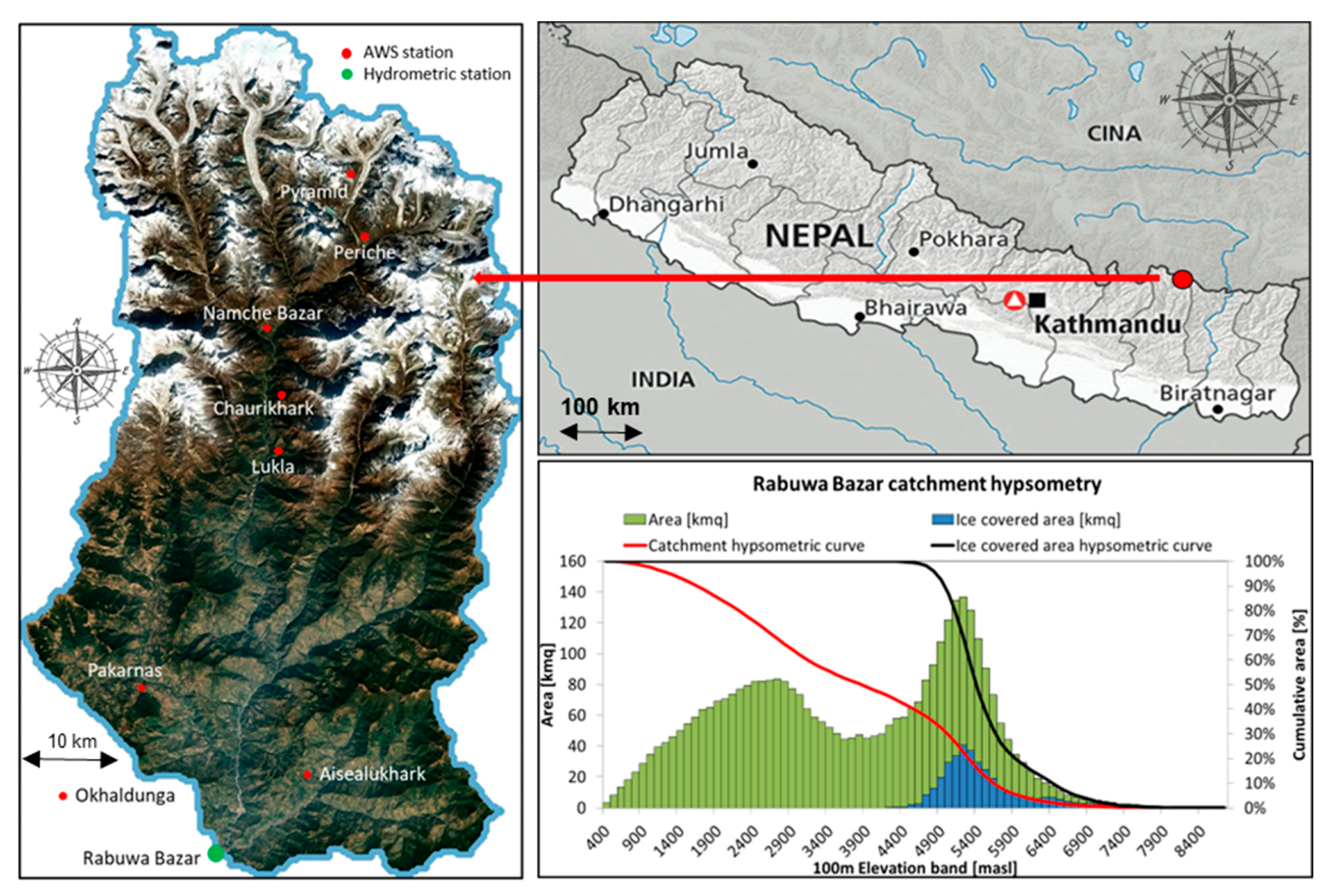
2. Case Study Area
3. Data Base
3.1. Topography, Land Use, and Hydrological Data
3.2. Demographic Data
4. Methods
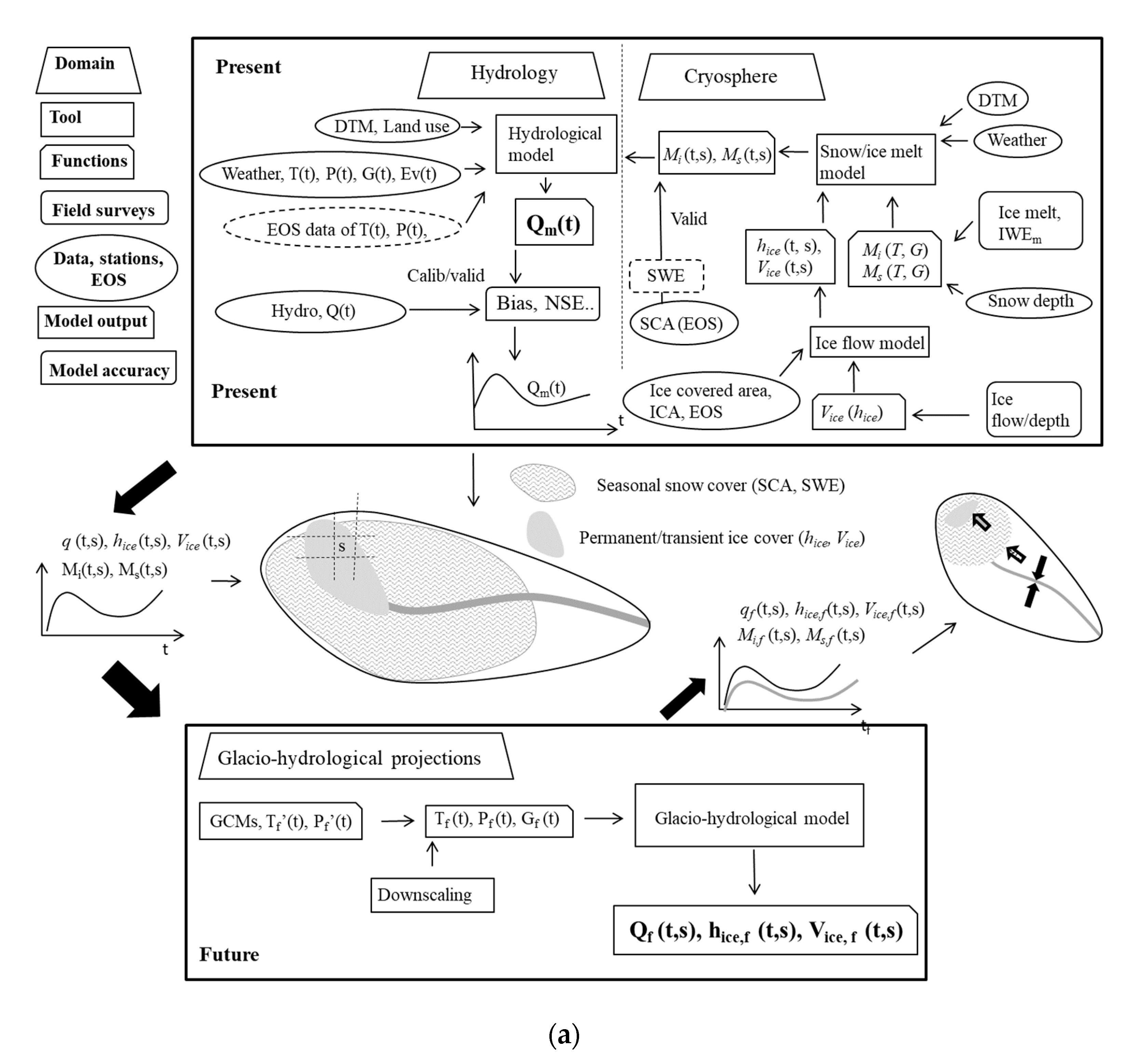
4.1. Hydrological Model
4.2. Energy Demand
4.3. Plants’ Design
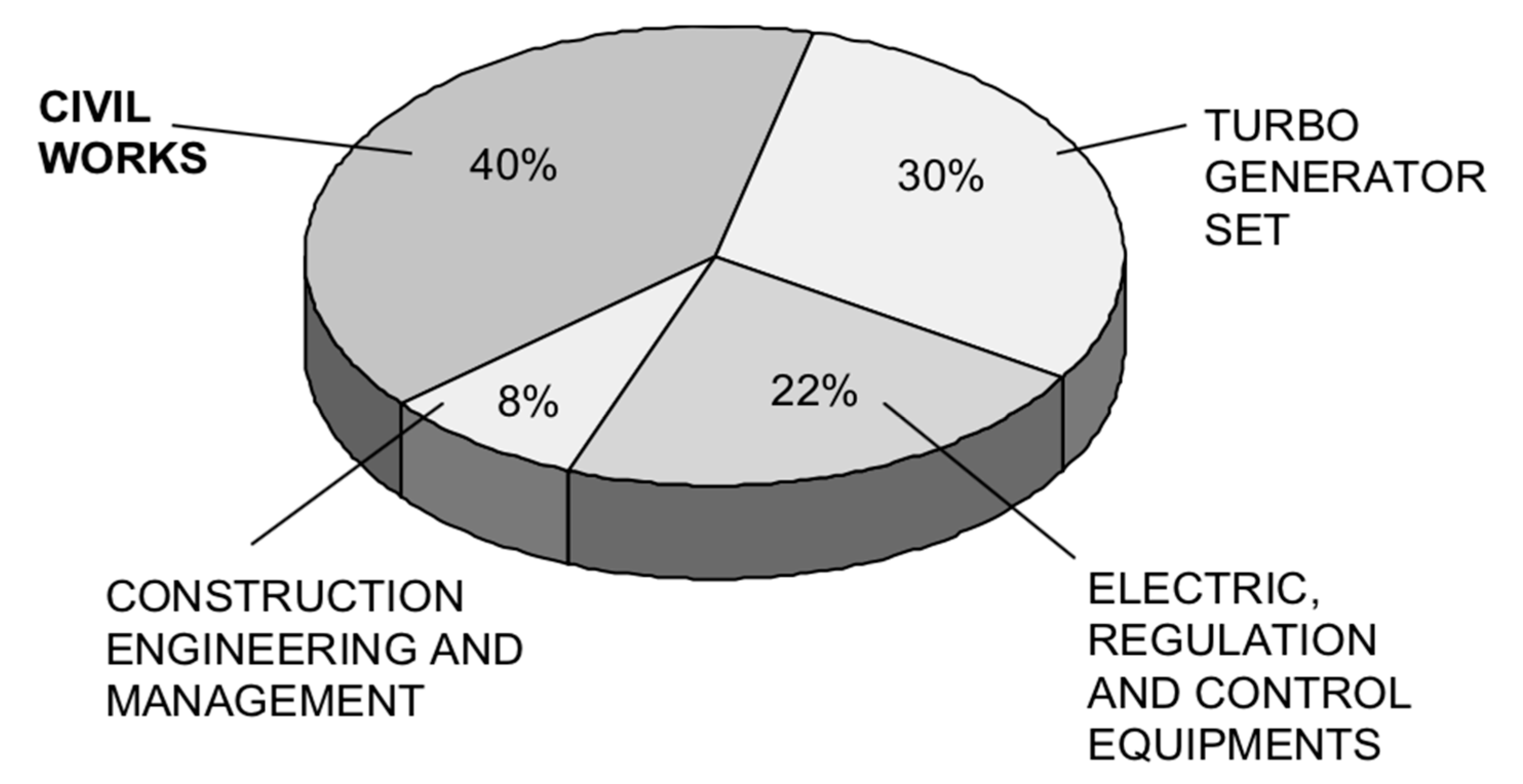
4.4. Cost Estimation
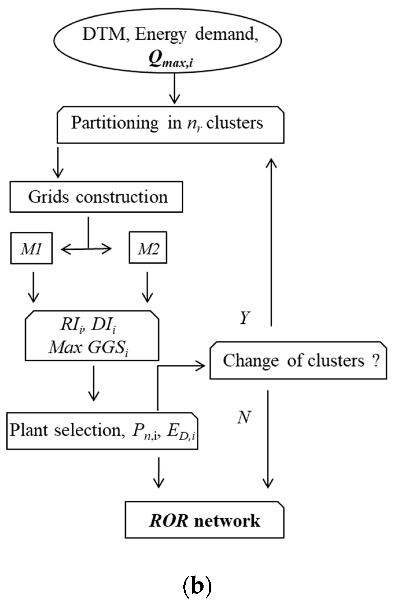
4.5. Heuristic Network Design Procedure, Poli-ROR
4.6. Future Scenarios
5. Results
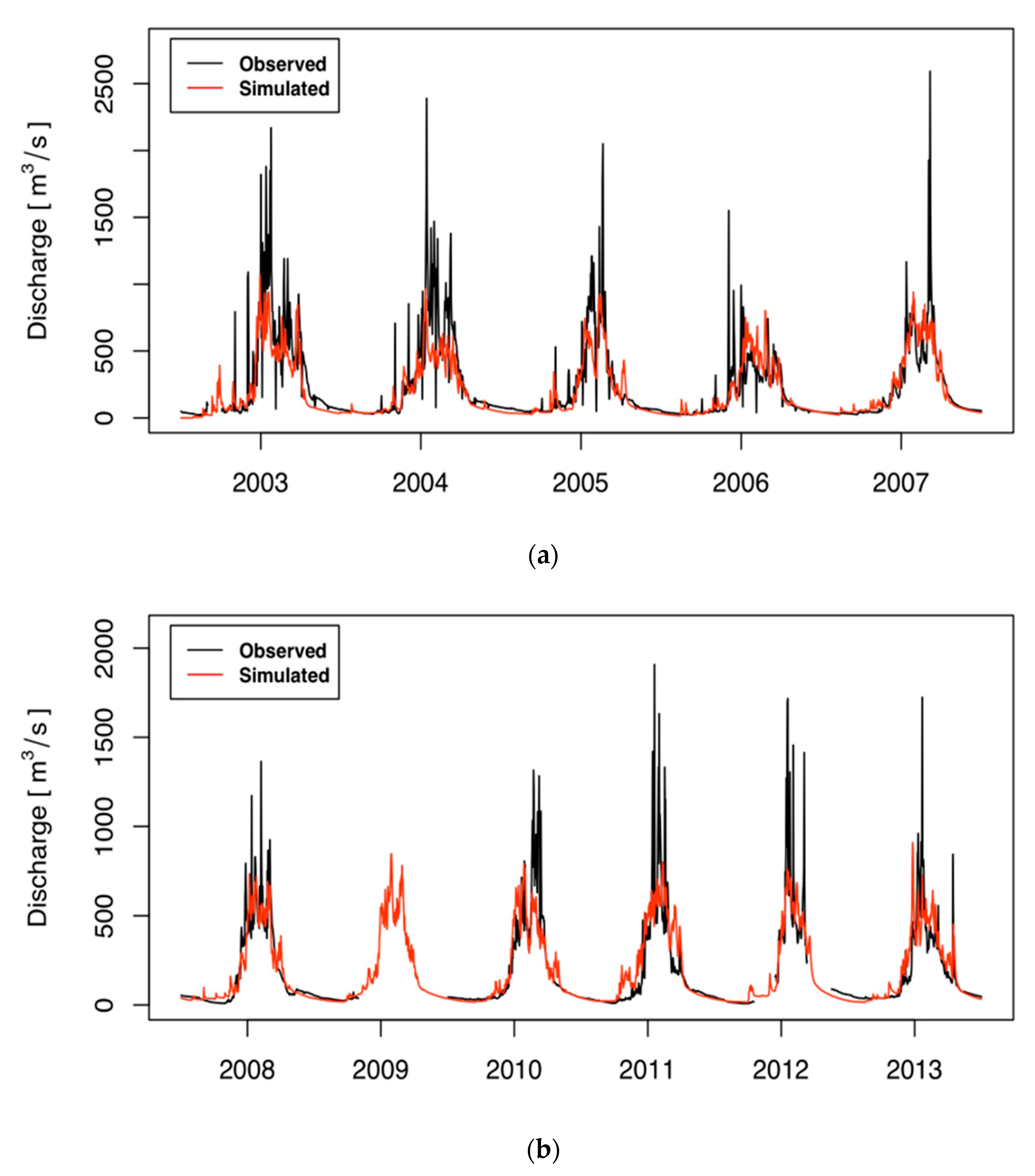
5.1. Poli-Hydro Model
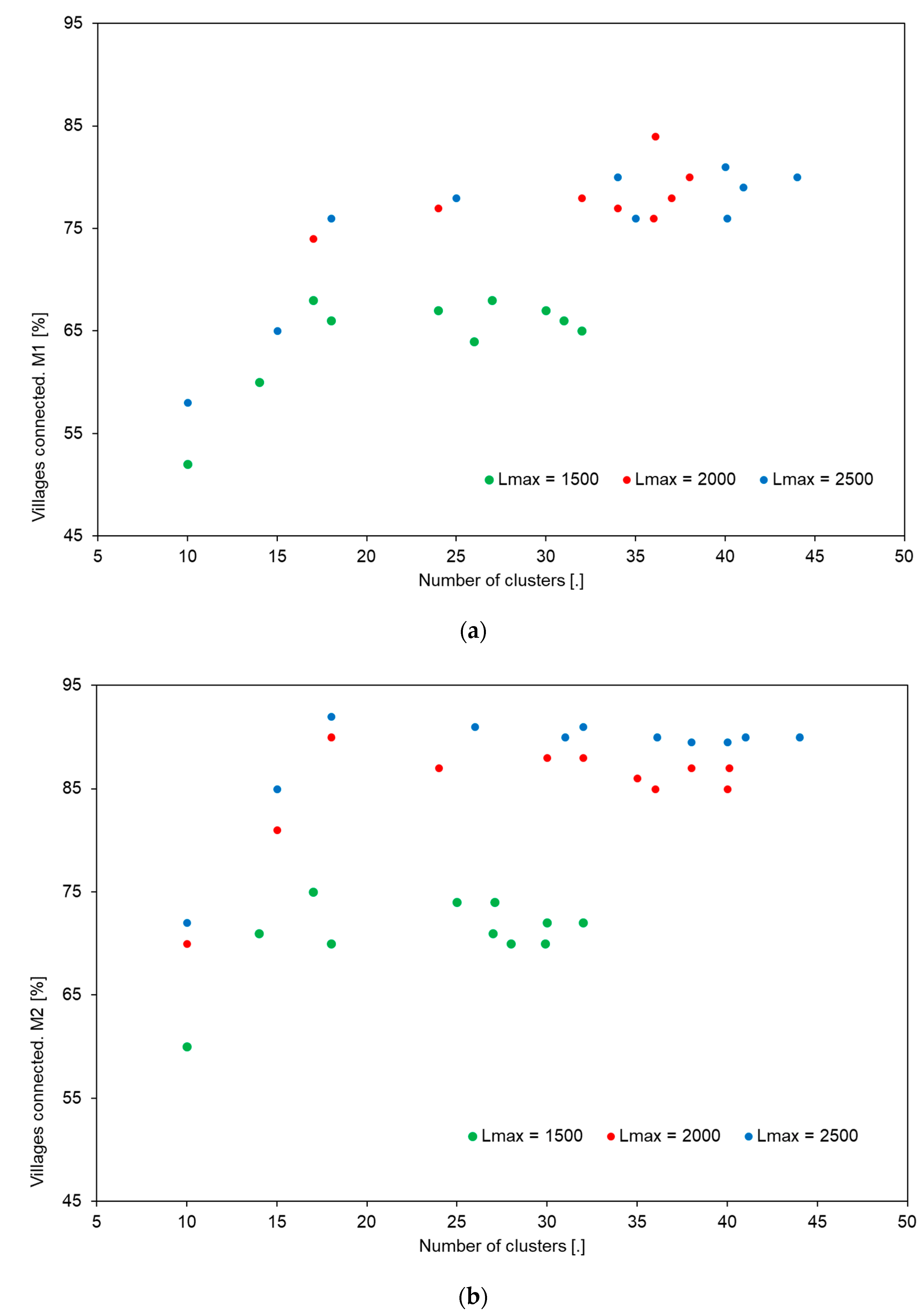
5.2. Poli-ROR
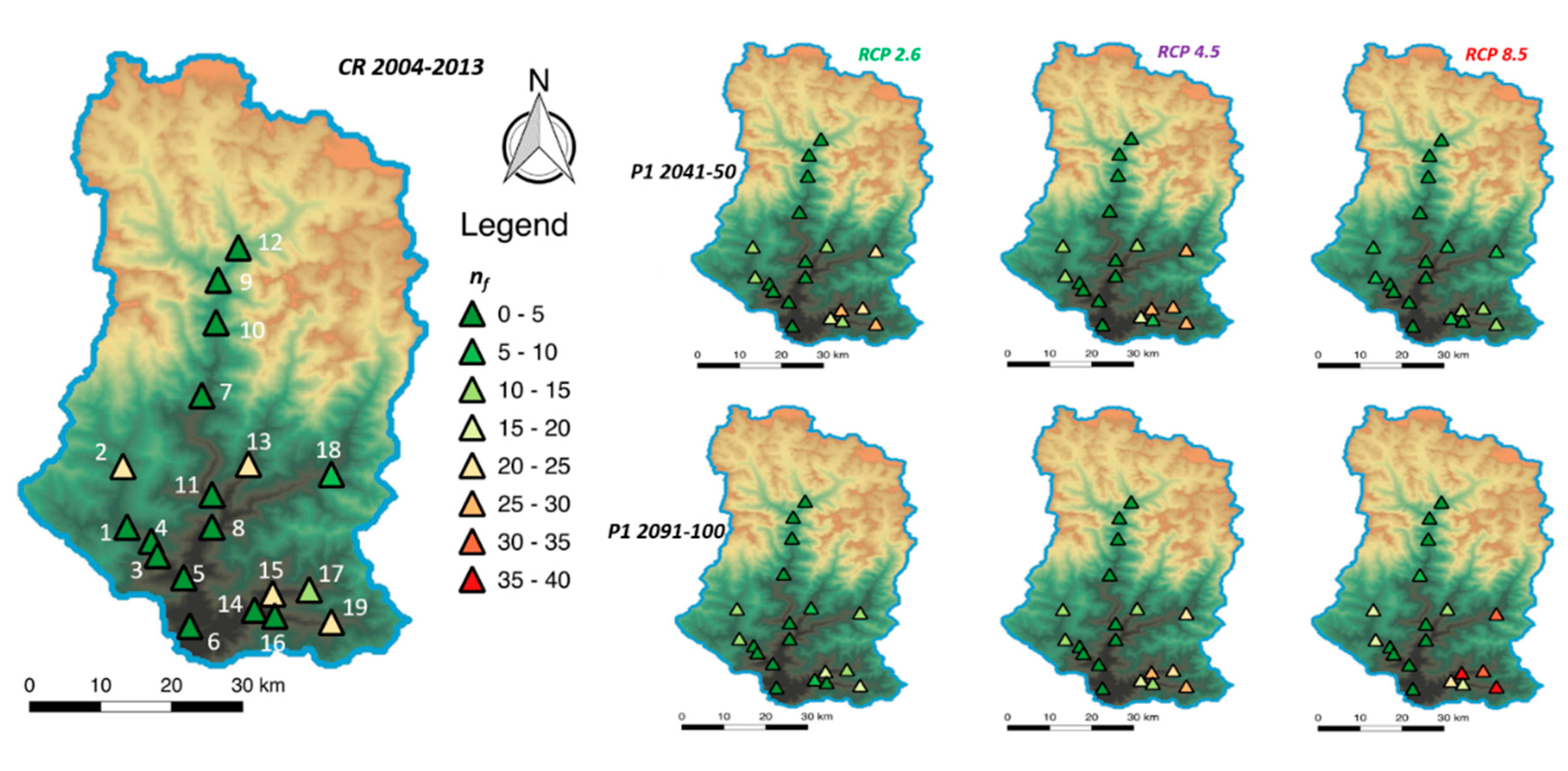
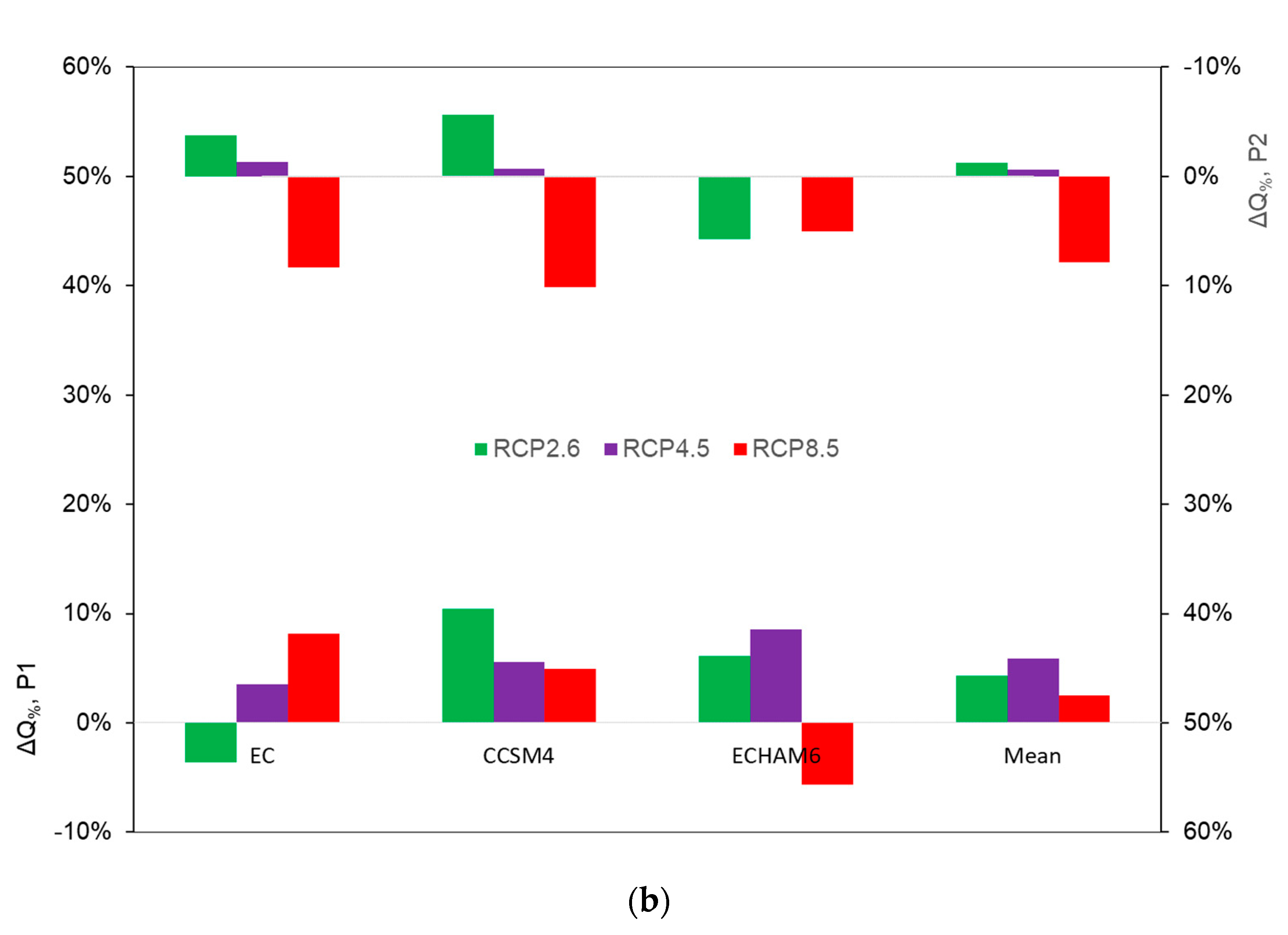
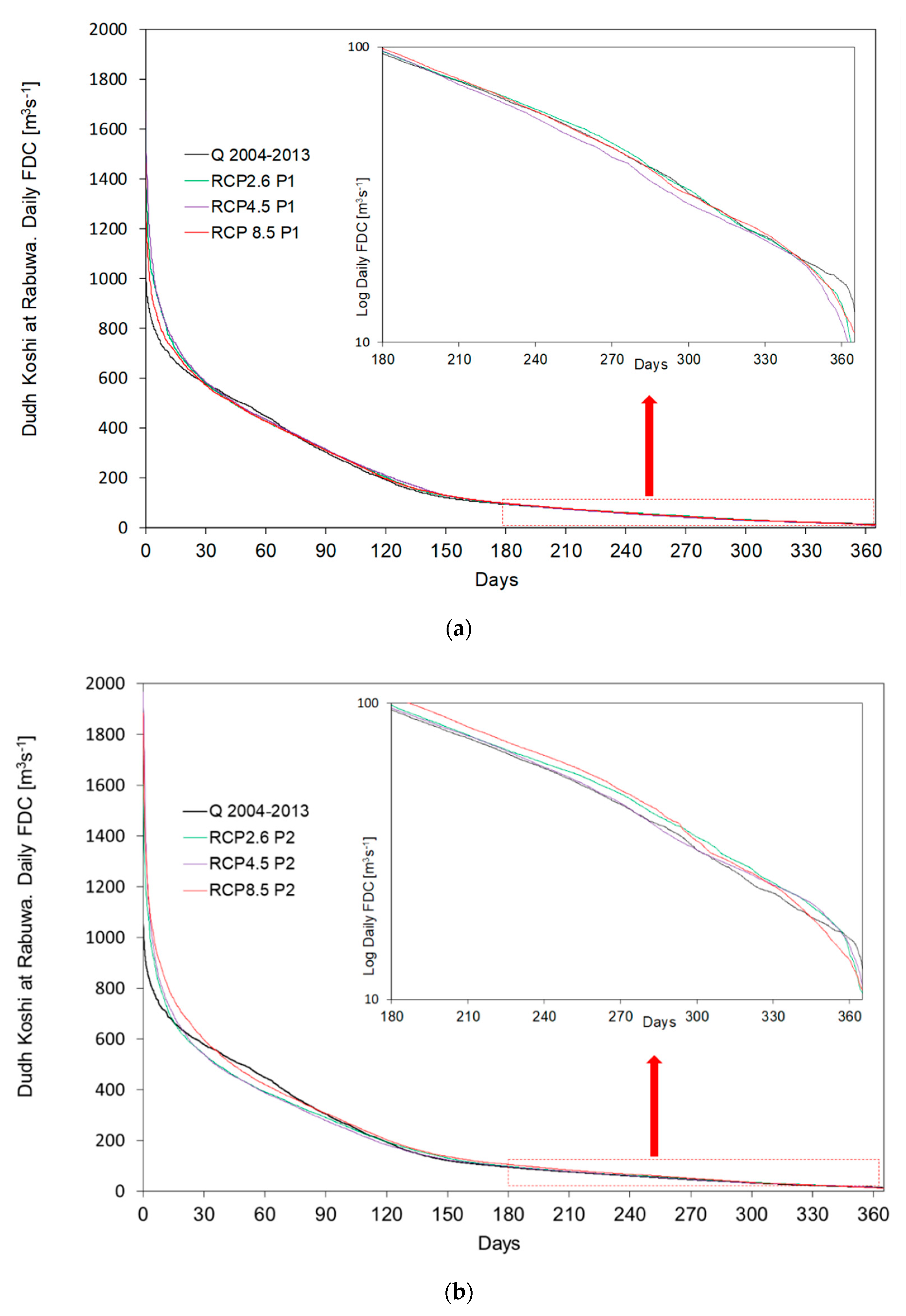
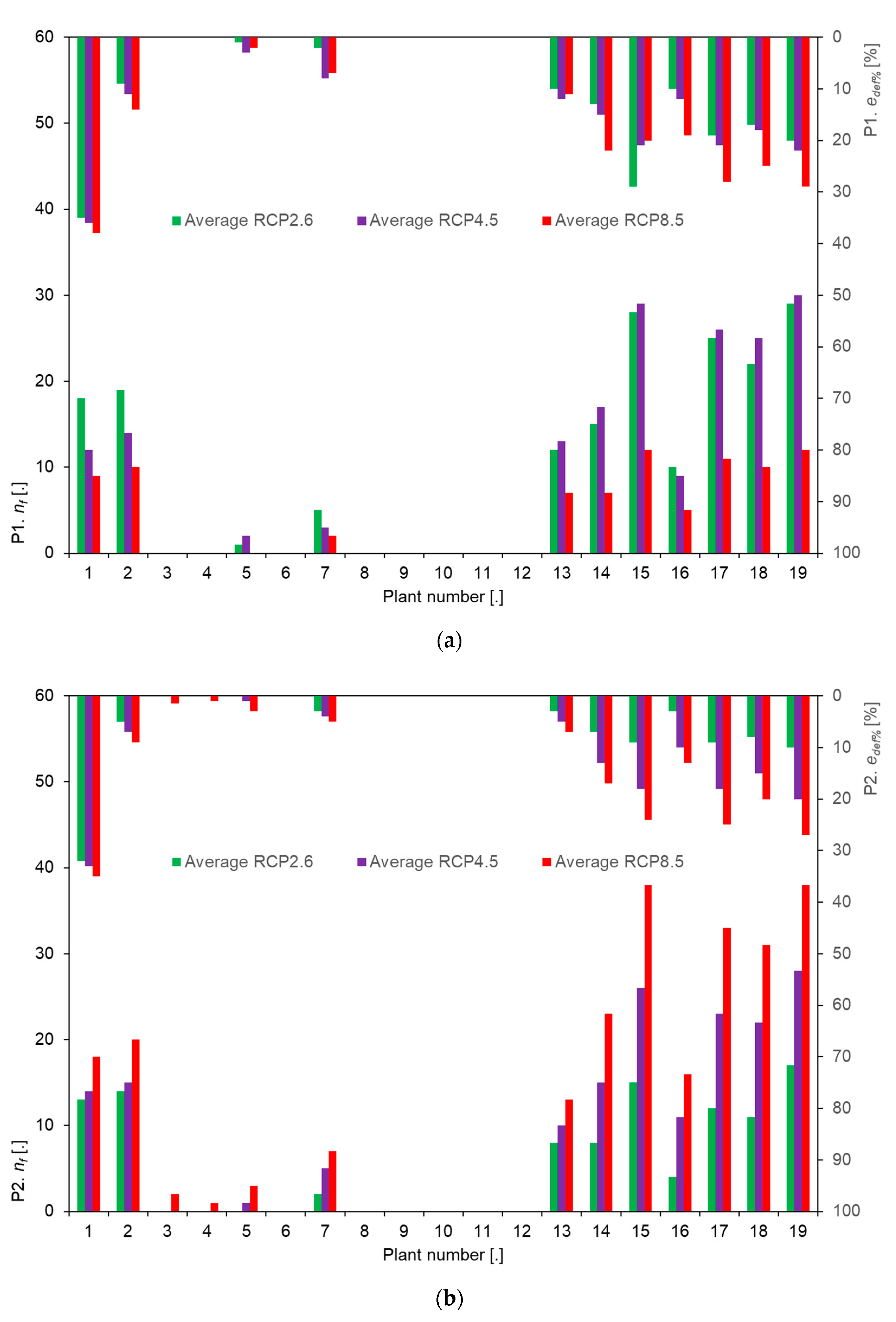
5.3. Future Flows, and Hydropower Potential
6. Discussion
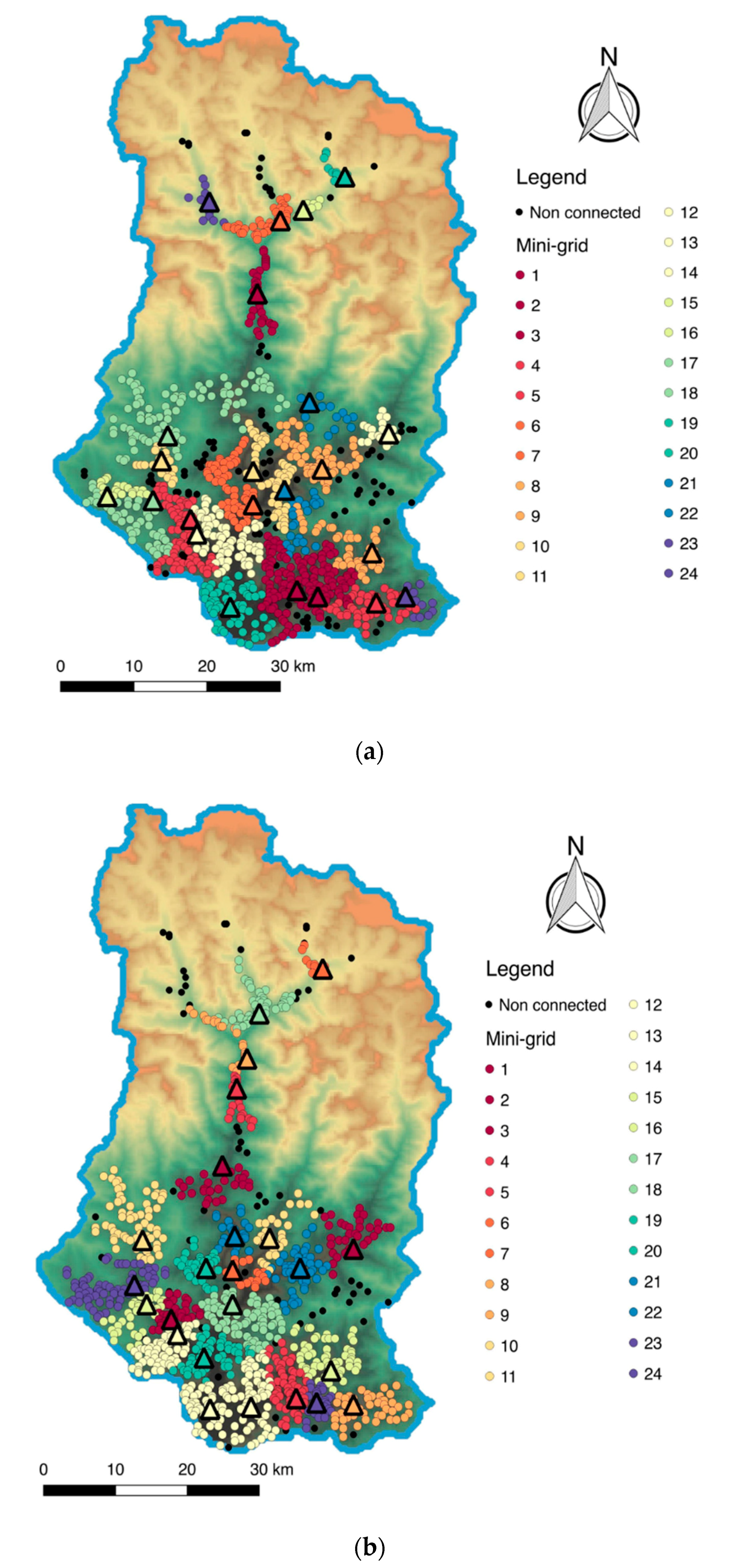
6.1. Improvement in Grid Design Using Poli-ROR
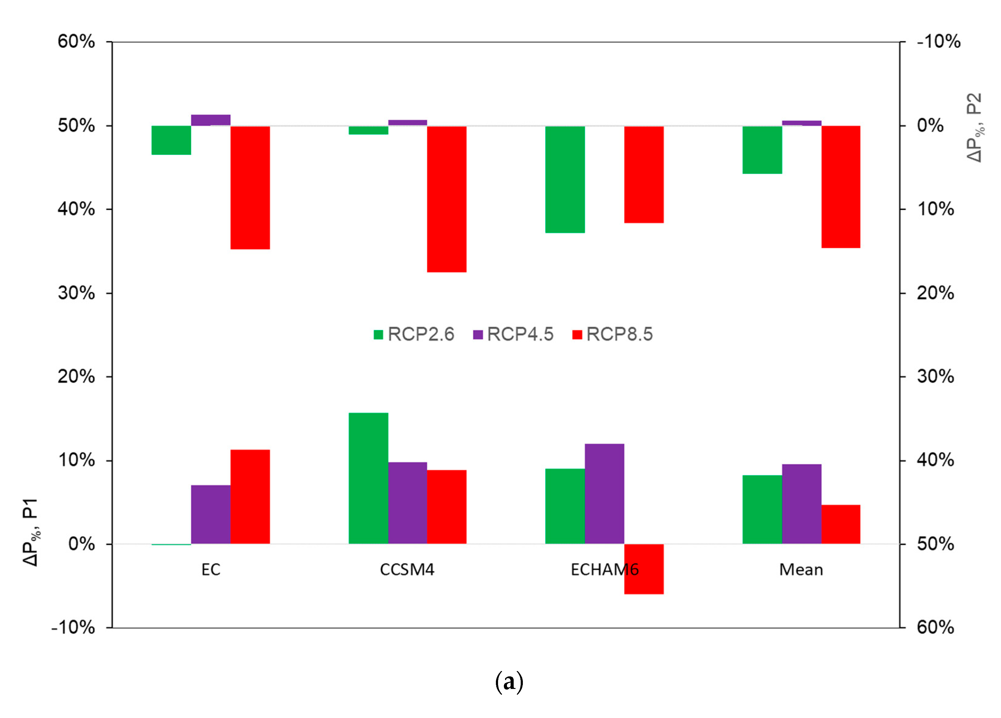
6.2. Potentially Modified Hydropower Potential under Climate Change
6.3. Limitations, and Outlooks
7. Conclusions
Author Contributions
Funding
Acknowledgments
Conflicts of Interest
References
- United Nations Organization. The 2030 Agenda for Sustainable Development. Available online: https://www.un.org/ga/search/view_doc.asp?symbol=A/RES/70/1&Lang=E (accessed on 18 September 2020).
- International Energy Agency IEA. Special Report: Energy Access Outlook; IEA: Paris, France, 2017. [Google Scholar]
- Nerini, F.F.; Broad, O.; Mentis, D.; Welsch, M.; Bazilian, M.; Howells, M. A cost comparison of technology approaches for improving access to electricity services. Energy 2016, 95, 255–265. [Google Scholar] [CrossRef]
- IRENA. Innovation Outlook Renewable Mini-grids. 2016. Available online: https://www.irena.org/publications/2016/Sep/Innovation-Outlook-Renewable-mini-grids (accessed on 18 September 2020).
- Karki, R.; Gurung, A. An Overview of Climate Change And Its Impact on Agriculture: A Review From Least Developing Country, Nepal. Int. J. Ecosyst. 2012, 2, 19–24. [Google Scholar] [CrossRef] [Green Version]
- OXFAM. Even the Himalayas Have Stopped Smiling: Climate Change, Poverty and Adaptation in Nepal; Oxfam International, Country Programme Office: Lalitpur, Nepal, 2009. [Google Scholar]
- Immerzeel, W.W.; van Beek, L.P.H.; Bierkens, M.F.P. Climate Change Will Affect the Asian Water Towers. Science 2010, 328, 1382–1385. [Google Scholar] [CrossRef] [PubMed]
- Immerzeel, W.; Petersen, L.; Ragettli, S.; Pellicciotti, F. The importance of observed gradients of air temperature and precipitation for modeling runoff from a glacierized watershed in the Nepalese Himalayas. Water Resour. Res. 2014, 50, 2212–2226. [Google Scholar] [CrossRef] [Green Version]
- Bocchiola, D. Agriculture and food security under climate change in Nepal. Adv. Plants Agric. Res. 2017, 6. [Google Scholar] [CrossRef] [Green Version]
- Konar, M.; Dalin, C.; Suweis, S.; Hanasaki, N.; Rinaldo, A.; Rodriguez-Iturbe, I. Water for food: The global virtual water trade network. Water Resour. Res. 2011, 47, W05520. [Google Scholar] [CrossRef] [Green Version]
- Palazzoli, I.; Maskey, S.; Uhlenbrook, S.; Nana, E.; Bocchiola, D. Impact of prospective climate change upon water resources and crop yield in the Indrawati basin, Nepal. Agric. Syst. 2015, 133C, 143–157. [Google Scholar] [CrossRef]
- Chalise, S.R.; Kansakar, S.R.; Rees, G.; Croker, K.; Zaidman, M. Management of water resources and low flow estimation for the Himalayan basins of Nepal. J. Hydrol. 2003, 282, 25–35. [Google Scholar] [CrossRef]
- Rees, H.G.; Holmes, M.G.R.; Fry, M.J.; Young, A.R.; Pitson, D.G.; Kansakar, S.R. An integrated water resource management tool for the Himalayan region. Environ. Modell. Softw. 2006, 21, 1001–1012. [Google Scholar] [CrossRef]
- Mainali, B.; Silveira, S. Financing off-grid rural electrification: Country case. Nepal Energy 2011, 36, 2194–2201. [Google Scholar] [CrossRef]
- Sangroula, D.P. Hydropower development and its sustainability with respect to sedimentation in Nepal. J. Inst. Eng. 2009, 7, 1–9. [Google Scholar] [CrossRef] [Green Version]
- Nepal, R. Roles and potentials of renewable energy in less-developed economies: The case of Nepal. Renew. Sustain. Energy Rev. 2012, 16, 2200–2206. [Google Scholar] [CrossRef]
- Sanchez, T.; Dennis, R.; Pullen, K.R. Cooking and lighting habits in rural Nepal and Uganda. J. Power Energy 2013, 227, 727–739. [Google Scholar] [CrossRef]
- Houghton, J.T.; Ding, Y.; Griggs, D.J.; Noguer, M.; van der Linden, P.J.; Dai, X.; Maskell, K.; Johnson, C.A. Contribution of working group I to the third assessment report of the intergovernmental panel on climate change. In Climate Change 2001: The Scientific Basis; Cambridge University Press: Cambridge, UK, 2001. [Google Scholar]
- Parajuli, I.; Lee, H.; Shrestha, K.R. Indoor air quality and ventilation assessment of rural mountainous households of Nepal. Int. J. Sustain. Built Environ. 2016, 5, 301–311. [Google Scholar] [CrossRef] [Green Version]
- Pokharel, S. Kyoto protocol and Nepal’s energy sector. Energy Policy 2007, 35, 2514–2525. [Google Scholar] [CrossRef]
- Sharma, C.K. Overview of Nepal’s energy sources and environment. Atmospheric Environ. 1996, 30, 2717–2720. [Google Scholar] [CrossRef]
- Soncini, A.; Bocchiola, D.; Confortola, G.; Minora, U.; Vuillermoz, E.; Salerno, F.; Viviano, G.; Shrestha, D.; Senese, A.; Smiraglia, C.; et al. Future hydrological regimes and glacier cover in the Everest region: The case study of the Dudh Koshi basin. Sci. Total Environ. 2016, 565, 1084–1095. [Google Scholar] [CrossRef] [Green Version]
- Thakuri, S.; Salerno, F.; Smiraglia, C.; Bolch, T.; D’Agata, C.; Viviano, G.; Tartari, G. Tracing glacier changes since the 1960s on the south slope of Mt. Everest (central Southern Himalaya) using optical satellite imagery. Cryosphere 2014, 8, 1297–1315. [Google Scholar] [CrossRef] [Green Version]
- Devkota, L.P.; Gyawali, D.R. Impacts of climate change on hydrological regime and water resources management of the Koshi River Basin. Nepal J. Hydrol. Reg. Stud. 2015, 4, 502–515. [Google Scholar] [CrossRef] [Green Version]
- Bocchiola, D.; Soncini, A. Water resources modeling and prospective evaluation in the Indus River under present and prospective climate change. In Indus River Basin: Water Security and Sustainability; Khan, S., Adams, T., Eds.; Elsevier: Amsterdam, The Netherlands, 2019; p. 500. ISBN 9780128127827. [Google Scholar]
- Gautam, B.R.; Li, F.; Ru, G. Climate Change Risk for Hydropower Schemes in Himalayan Region. Environ. Sci. Technol. 2014, 48, 7702–7703. [Google Scholar] [CrossRef]
- Hussain, A.; Sarangi, G.K.; Pandit, A.; Ishaq, S.; Mamnun, N.; Ahmad, B.; Jamil, M.K. Hydropower development in the Hindu Kush Himalayan region: Issues, policies and opportunities. Renew. Sustain. Energy Rev. 2019, 107, 446–461. [Google Scholar] [CrossRef]
- Mishra, S.K.; Hayse, J.; Veselka, T.; Yan, E.; Kayastha, R.B.; LaGory, K.; McDonald, K.; Steiner, N. An integrated assessment approach for estimating the economic impacts of climate change on River systems: An application to hydropower and fisheries in a Himalayan River, Trishuli. Environ. Sci. Policy 2018, 87, 102–111. [Google Scholar] [CrossRef]
- Agarwal, A.; Babel, M.S.; Maskey, S. Analysis of future precipitation in the Koshi River basin, Nepal. J. Hydrol. 2014. [Google Scholar] [CrossRef]
- Awasthi, K.D.; Sitaula, B.K.; Singh, B.R.; Bajacharaya, R.M. Land-use change in two Nepalese watersheds: GIS and geomorphometric analysis. Land Degrad. Dev. 2002, 13, 495–513. [Google Scholar] [CrossRef]
- Chhetri, N.; Chaudhary, P.; Tiwari, P.R.; Yadaw, R.B. Institutional and technological innovation: Understanding agricultural adaptation to climate change in Nepal. Appl. Geogr. 2012, 33, 142–150. [Google Scholar] [CrossRef]
- Eriksson, M.; Xu, J.C.; Shrestha, A.B.; Vaidya, R.A.; Santosh, N.; Sandström, K. The Changing Himalayas: Impact of Climate Change on Water Resources and Livelihoods in the Greater Himalayas; ICIMOD: Kathmandu, Nepal, 2009; p. 29. ISBN 978-92-9115-111-0. [Google Scholar]
- Gentle, P.; Maraseni, T.N. Climate change, poverty and livelihoods: Adaptation practices by rural mountain communities in Nepal. Environ. Sci. Pol. 2012, 21, 24–34. [Google Scholar] [CrossRef]
- Maskey, S.; Uhlenbrook, S.; Ojha, S. An analysis of snow cover changes in the Himalayan region using MODIS snow products and in-situ temperature data. Clim. Chang. 2011, 108, 391–400. [Google Scholar] [CrossRef]
- Nyaupanea, G.P.; Chhetri, N. Vulnerability to Climate Change of Nature-Based Tourism in the Nepalese Himalayas. Tour. Geogr. 2009, 11, 95–119. [Google Scholar] [CrossRef]
- Rai, M. Climate change and agriculture: A Nepalese case. J. Agric. Environ. 2007, 8, 92–95. [Google Scholar] [CrossRef]
- Shrestha, A.B.; Aryal, R. Climate change in Nepal and its impact on Himalayan glaciers. Reg. Environ. Chang. 2011, 11, 65–77. [Google Scholar] [CrossRef]
- Dulal, H.B.; Brodnig, G.; Thakur, H.K.; Green-Onoriose, C. Do the poor have what they need to adapt to climate change? A case study of Nepal. Local Environ. 2010, 15, 621–635. [Google Scholar] [CrossRef]
- USAID. Nepal Climate Vulnerability Profile; USAID: Washington, DC, USA, 2012.
- WECS. Energy Sector Synopsis Report; WECS: Kathmandu, Nepal, 2016. [Google Scholar]
- Jha, R. Total Run-of-River type Hydropower Potential of Nepal. Hydro-Nepal 2010, 7, 8–13. [Google Scholar] [CrossRef]
- Gianinetto, M.; Polinelli, F.N.; Frassy, F.; Aiello, M.; Rota Nodari, F.; Soncini, A.; Bocchiola, D. Analysis of changes in crop farming in the Dudh Koshi (Nepal) driven by climate changes. In Proceedings of the Earth Resources and Environmental Remote Sensing/GIS Applications, Warsaw, Poland, 5 October 2014. [Google Scholar] [CrossRef]
- Bocchiola, D.; Brunetti, L.; Soncini, A.; Polinelli, F.; Gianinetto, M. Impact of climate change on agricultural productivity and food security in the Himalayas: A case study in Nepal. Agric. Syst. 2019, 171, 113–125. [Google Scholar] [CrossRef]
- FAO. Food and Nutrition Security in Nepal: A Status Report—Ministry of Agricultural Development and Central Bureau of Statistics for the Nepal Component of the FSO Project; FAO: Rome, Italy, 2016; Available online: http://admin.indiaenvironmentportal.org.in/files/file/Food%20and%20Nutrition%20Security%20in%20Nepal.pdf (accessed on 18 September 2020).
- Vuillermoz, E.; Cristofanelli, P. Atmospheric Brown Clouds in the Himalayas: First two years of continuous observations at the Nepal Climate Observatory-Pyramid (5079 m). Atmos. Chem. Phys. 2010, 10, 7515–7531. [Google Scholar]
- Government of Nepal, National Planning Commission Secretariat, Central Bureau of Statistics National Population and Housing Census 2011 (National Report). 2012. Available online: https://unstats.un.org/unsd/demographic-social/census/documents/Nepal/Nepal-Census-2011-Vol1.pdf (accessed on 18 September 2020).
- Neupane, N.; Ramachandra Murthy, M.S.; Rasul, G.; Wahid, S.; Shrestha, A.B.; Uddin, K. Integrated Biophysical and Socioeconomic Model for Adaptation to Climate Change for Agriculture and Water in the Koshi Basin. In Handbook of Climate Change Adaptation; Springer: Berlin, Germany, 2013. [Google Scholar]
- Sahas Urja. Solu Khola (Dudhkoshi) Hydro-Electric Project—86MW. Salient Features. 2018. Available online: http://sahasurja.com/project/solu-khola-dudhkoshi-hydro-electric-project-86mw/ (accessed on 18 September 2020).
- Soncini, A.; Bocchiola, D.; Azzoni, R.S.; Diolaiuti, G. A methodology for monitoring and modeling of high altitude Alpine catchments. Prog. Phys. Geogr. 2017, 41, 393–420. [Google Scholar] [CrossRef]
- Shea, J.M.; Immerzeel, W.W.; Wagnon, P.; Vincent, C.; Bajracharya, S. Modelling glacier change in the Everest region, Nepal Himalaya. Cryosphere 2015, 9, 1105–1128. [Google Scholar] [CrossRef] [Green Version]
- Peel, M.C.; Finlayson, B.L.; McMahon, T.A. Updated world map of the Köppen-Geiger climate classification. Hydrol. Earth Syst. Sci. 2007, 11, 1633–1644. [Google Scholar] [CrossRef] [Green Version]
- WWF, World Wildlife Fund, Nepal. Water Poverty of Indrawati Basin, Analysis and Mapping, June 2012; WWF: Kathmandu, Nepal, 2012; Available online: http://awsassets.panda.org/downloads/water_poverty_book.pdf (accessed on 18 September 2020).
- Cook, S.; Rubiano, J.; Sullivan, C.; Andah, W.; Ashante, F.; Wallace, J.; Terrasson, I.; Nikiema, A.; Kemp-Benedict, E.; Tourino, I.; et al. Water poverty mapping in the Volta basin. In Proceedings of the CGIAR Challenge program on water and food, Workshop report, Accra, Ghana, 3–8 March 2007; Available online: http://cpwfbfp.pbworks.com/f/Water_poverty_mapping_Volta_Ghana_Workshop_Report.pdf (accessed on 18 September 2020).
- NAPA. National Adaptation Programme of Action (NAPA); Government of Nepal, Ministry of Environment: Kathmandu, Nepal, 2010.
- ICIMOD. Nepal’s Digital Agriculture Atlas; ICIMOD: Kathmandu, Nepal, 2015; Available online: http://geoportal.icimod.org/?q=21298 (accessed on 18 September 2020).
- FAO. The Soil and Terrain database (SOTER) for Nepal. 2004. Available online: http://www.fao.org/soils-portal/soil-survey/soil-maps-and-databases/regional-and-national-soil-maps-and-databases/en/ (accessed on 18 September 2020).
- Higuchi, K.; Ageta, Y.; Yasunari, T.; Inoue, J. Characteristics of precipitation during the monsoon season in high-mountain areas of the Nepal Himalaya. Hydrol. Asp. Alp. High-Mt. Areas 1982, 138, 21–30. [Google Scholar]
- Salerno, F.; Guyennon, N.; Thakuri, S.; Viviano, G.; Romano, E.; Vuillermoz, E.; Cristofanelli, P.; Stocchi, P.; Agrillo, G.; Ma, Y.; et al. Weak precipitation, warm winters and springs impact glaciers of south slopes of Mt. Everest (central Himalaya) in the last 2 decades (1994–2013). Cryosphere 2015, 9, 1229–1247. [Google Scholar] [CrossRef] [Green Version]
- Bocchiola, D. Use of Scale Recursive Estimation for multi-sensor rainfall assimilation: A case study using data from TRMM (PR and TMI) and NEXRAD. Adv. Water Resour. 2007, 30, 2354–2372. [Google Scholar] [CrossRef]
- Bookhagen, B. High resolution spatiotemporal distribution of rainfall seasonality and extreme events based on a 12-year TRMM time series. 2012. Available online: http://www.geog.ucsb.edu/~bodo/pdf/bookhagen_global_TRMM_extremeE_DR_final.pdf (accessed on 18 September 2020).
- Bocchiola, D.; Soncini, A.; Senese, A.; Diolaiuti, G. Modelling hydrological components of the Rio Maipo of Chile, and their prospective evolution under climate change. Climate 2018, 6, 57. [Google Scholar] [CrossRef] [Green Version]
- OCHA, Office for the Coordination of Humanitarian Affairs, Nepal. 2015. Available online: https://www.unocha.org/asia-and-pacific-roap/nepal (accessed on 18 September 2020).
- Worldpop. Open spatial demographic data. Available online: https://www.worldpop.org/.2015 (accessed on 18 September 2020).
- Stevens, F.R.; Gaughan, A.E.; Linard, C.; Tatem, A.J. Disaggregating Census Data for Population Mapping Using Random Forests with Remotely-Sensed and Ancillary Data. PLoS ONE 2015, 10, e0107042. [Google Scholar] [CrossRef] [PubMed] [Green Version]
- Siddaiah, R.; Saini, R.P. A review on planning, configurations, modeling and optimization techniques of hybrid renewable energy systems for off-grid applications. Renew. Sustain. Energy Rev. 2016, 58, 376–396. [Google Scholar] [CrossRef]
- Soncini, A.; Bocchiola, D.; Confortola, G.; Bianchi, A.; Rosso, R.; Mayer, C.; Lambrecht, A.; Palazzi, E.; Smiraglia, C.; Diolaiuti, G. Future hydrological regimes in the Upper Indus basin: A case study from a high-altitude glacierized catchment. J. Hydrometeorol. 2015, 16, 306–326. [Google Scholar] [CrossRef] [Green Version]
- Aili, T.; Soncini, A.; Bianchi, A.; Diolaiuti, G.; D’Agata, C.; Bocchiola, D. Assessing water resources under climate change in high-altitude catchments: A methodology and an application in the Italian Alps. Appl. Clim. 2018, 135, 1–22. [Google Scholar] [CrossRef]
- Oerlemans, J. Glaciers and Climate Change; A.A. Balkema Publishers: Brookfield, VT, USA, 2001; p. 148. [Google Scholar]
- Haeberli, W.; Hölzle, M. Application of inventory data for estimating characteristics of and regional climate-change effects on mountain glaciers: A pilot study with the European Alps. Ann. Glaciol. 1995, 21, 206–212. [Google Scholar] [CrossRef] [Green Version]
- Rosso, R. Nash model relation to Horton order ratios. Water Resour. Res. 1984, 20, 914–920. [Google Scholar] [CrossRef]
- Shrestha, S.; Khatiwada, M.; Babel, M.S.; Parajuli, K. Impact of Climate Change on River Flow and Hydropower Production in Kulekhani Hydropower Project of Nepal. Environ. Process. 2014, 1, 231–250. [Google Scholar] [CrossRef] [Green Version]
- International Energy Agency IEA. Nepal Energy Balance Flow; IEA: Paris, France, 2015. [Google Scholar]
- Proietti, S.; Sdringola, P.; Castellani, F.; Astolfi, D.; Vuillermoz, E. On the contribution of renewable energies for feeding a high altitude Smart Mini Grid. Appl. Energy 2017, 185, 15–20. [Google Scholar] [CrossRef]
- Salerno, F.; Viviano, G.; Mangredi, E.C.; Caroli, P.; Thakuri, S.; Tartari, G. Multiple Carrying Capacities from a management-oriented perspective to operationalize sustainable tourism in protected area. J. Environ. Manag. 2013, 128, 116–125. [Google Scholar] [CrossRef]
- ICIMOD. Regional Data Base Initiative; ICIMOD: Kathmandu, Nepal, 2017; Available online: http://www.icimod.org/?q=rdi (accessed on 18 September 2020).
- Ogayar, B.; Vidal, P.G. Cost determination of the electro-mechanical equipment of a small hydro-power plant. Renew. Energy 2009, 34, 6–13. [Google Scholar] [CrossRef]
- Silver, E. An overview of heuristic solution methods. J. Oper. Res. Soc. 2004, 55, 936–956. [Google Scholar] [CrossRef]
- Ranaboldo, M.; Ferrer Martì, L.; Garcia-Villoria, A.; Moreno, R.P. Heuristic indicators for the design of community off-grid electrification systems based on multiple renewable energies. Energy 2013, 50, 501–512. [Google Scholar] [CrossRef]
- Ranaboldo, M.; Garcia-Villoria, A.; Ferrer-Martì, L.; Moreno, R.P. A heuristic method to design autonomous village electrification projects with renewable energies. Energy 2014, 73, 96–109. [Google Scholar] [CrossRef]
- Ranaboldo, M.; Garcia-Villoria, A.; Ferrer-Martì, L.; Moreno, R.P. A meta-heuristic method to design off-grid community electrification projects with renewable energies. Energy 2015, 93, 2467–2482. [Google Scholar] [CrossRef] [Green Version]
- Groppelli, B.; Soncini, A.; Bocchiola, D.; Rosso, R. Evaluation of future hydrological cycle under climate change scenarios in a mesoscale Alpine watershed of Italy. Nat. Haz. Earth Sys. Sci. 2011, 11, 1769–1785. [Google Scholar] [CrossRef] [Green Version]
- Stevens, B.; Giorgetta, M.; Esch, M.; Mauritsen, T.; Crueger, T.; Rast, S.; Salzmann, M.; Schmidt, H.; Bader, J.; Block, K.; et al. Atmospheric component of the MPI-M Earth System Model: ECHAM6. J. Adv. Model. Earth Syst. 2013, 5, 1–27. [Google Scholar] [CrossRef]
- Gent, P.R.; Danabasoglu, G.; Donner, L.J.; Holland, M.M.; Hunke, E.C.; Jayne, S.R.; Lawrence, D.M.; Neale, R.B.; Rasch, P.J.; Vertenstein, M.; et al. The Community Climate System Model Version 4. J. Clim. 2011, 24, 4973–4991. [Google Scholar] [CrossRef]
- Hazeleger, W.; Wang, X.; Severijns, C.; Ştefănescu, S.; Bintanja, R.; Sterl, A.; Wyser, K.; Semmler, T.; Yang, S.; van den Hurk, B.; et al. EC-Earth V2.2: Description and validation of a new seamless earth system prediction model. Clim. Dyn. J. 2011, 39, 2611–2629. [Google Scholar] [CrossRef]
- Savéan, M.; Delclaux, F.; Chevallier, P.; Wagnon, P.; Gonga-Saholiariliva, N.; Sharma, R.; Neppel, L.; Arnaud, Y. Water budget on the Dudh Koshi River (Nepal): Uncertainties on precipitation. J. Hydrol. 2015, 531, 850–862. [Google Scholar] [CrossRef]
- Manara, M. Planning rural electrification with mini hydro-power systems in the Dudh Koshi basin (Nepal). Master’s Thesis, Politecnico di Milano, Milan, Italy, 2018. [Google Scholar]
- Bolch, T.; Shea, J.M.; Liu, S.; Azam, F.M.; Gao, Y.; Gruber, S.; Immerzeel, W.W.; Kulkarni, A.; Li, H.; Tahir, A.A.; et al. Status and change of the cryosphere. In The Hindu Kush Himalaya Assessment; Wester, P., Mishra, A., Mukherji, A., Shrestha, A.B., Eds.; Springer: Cham, Switzerland, 2019; pp. 209–255. [Google Scholar]
- Pathak, M. Climate Change: Uncertainty for Hydropower Development in Nepal. Hydro Nepal 2010, 6, 31–34. [Google Scholar] [CrossRef]
- Bombelli, G.M.; Soncini, A.; Bianchi, A.; Bocchiola, D. Potentially modified hydropower production under climate change in the Italian Alps. Hydrol. Process 2019. [Google Scholar] [CrossRef]
- Butler, C.; Rest, M. Calculating Risk, Denying Uncertainty: Seismicity and Hydropower Development in Nepal. Himalaya 2017, 37, 15–25. [Google Scholar]
- Huber, H. Hydropower in the Himalayan Hazardscape: Strategic Ignorance and the Production of Unequal Risk. Water 2019, 11, 414. [Google Scholar] [CrossRef]


| Station | Alt [m a.s.l.] | Variable | Period | Resolution | Data Source |
|---|---|---|---|---|---|
| Okhaldunga | 1720 | T | 1996–2013 | daily | DHM |
| Lukla | 2660 | T | 2003–2013 | hourly | EvK2-CNR |
| Namche | 3570 | T, P | 2003–2013 | hourly | EvK2-CNR |
| Periche | 4260 | T, P | 2003–2013 | hourly | EvK2-CNR |
| Pyramid | 5035 | T, P, HS | 2003–2013 | hourly | EvK2-CNR |
| Aisealukhark | 1924 | P | 1970–2013 | daily | DHM |
| Pakarnas | 2231 | P | 1970–2013 | daily | DHM |
| Chaurikhark | 2619 | P | 1970–2013 | daily | DHM |
| Rabuwa Bazar | 480 | Q | 2003–2013 | daily | DHM |
| Parameter | Description | Value | Method |
|---|---|---|---|
| Ts (°C) | rainfall/snowfall threshold | 0 | literature |
| DDFs (mm day−1 °C−1) | degree day factor snow | 3.5 | snow depth data |
| DDFi (mm day−1 °C−1) | degree day factor ice | 2.5 | snow depth data |
| SRFs (mm day−1 W−1 vm2) | radiation factor snow | 6.5 × 10⁻³ | snow depth data |
| SRFi (mm day−1 W−1 vm2) | radiation factor ice | 3.5 × 10⁻³ | snow depth data |
| αs | albedo snow | 0.7 | radiation data |
| αi | albedo ice | 0.4 | radiation data |
| K [mm day−1] | soil transmissivity as saturation | 1 | monthly flows volumes |
| kg | soil transmissivity exponent | 2 | monthly flows volumes |
| θw | water content wilting | 0.15 | literature |
| θl | water content field capacity | 0.35 | literature |
| θs | water content saturation | 0.45 | literature |
| tl,s (h) | lag time, surface | 240 | stream flows, timing |
| tl,g (h) | lag time, subsurface | 1200 | stream flows, timing |
| Household Type | Energy Demand (kWh day−1 HH−1) | Lighting (%) | Cooking (%) | Other (%) |
|---|---|---|---|---|
| Residential | 5.6 | 9 | 89 | 2 |
| Lodge (trekking season) | 11 | 9 | 89 | 2 |
| Lodge (rest of year) | 3.3 | 8 | 90 | 2 |
| Parameter | Description | Value |
|---|---|---|
| Lpenstock,max (m) | maximum penstock length | 1000 |
| Athreshold (km2) | minimum catchment area | 20 |
| Pnom,max (kW) | max maximum nominal power | 1500 |
| EDagr (kWh ab−1 day−1) | agricultural energy demand | 0.11 |
| EDres (kWh HH−1 day−1) | residential energy demand | 8.25 |
| EDlodge,trek (kWh HH−1 day−1) | trek lodges energy demand (trekking season) | 16.2 |
| EDlodge,winter (kWh HH−1 day−1) | winter lodges energy demand (winter season) | 9.36 |
| e% (%) | maximum head loss (%) 5 | 5 |
| ctrans (€ m−1) | transmission line cost | 9 |
| cdistr (€ m−1) | distribution line cost | 5 |
| cconn,HH (€ HH−1) | cost for connecting a household | 100 |
| ctransf (€ kV A−1) | transformers’ cost | 100 |
| cbatt battery cost (€ unit−1) | battery cost | 500 |
| Capacitybatt (Ah unit−1) | battery capacity | 225 |
| Vbatt (V) | battery voltage | 12 |
| eleloss (%) | transmission and distribution losses | 5 |
| r (%) | discount rate (%) | 5 |
| Lmax (m) | maximum transmission length | SA |
| nclusters | number of clusters | SA |
| α | weighting factors, RI, DI | SA |
| Indicator Period | Bias Monthly (%) | Bias Year (%) | NSE Daily | LnNSE Daily |
|---|---|---|---|---|
| CAL | +7 | +16 | 0.71 | 0.68 |
| VAL | −12 | 0 | 0.66 | 0.86 |
| Overall | −3 | +7 | 0.68 | 0.78 |
| ID | ∆Hgross (m) | Qmax (m3 s−1) | Pnom (kW) | Esupplied (MWh day−1) | Sd (km2) | Villages | LCOE (€ kWh−1) | nf (day) | edef% (%) |
|---|---|---|---|---|---|---|---|---|---|
| 1 | 69 | 1.79 | 1211 | 25.3 | 480 | 88 | 0.06 | 0 | 0 |
| 2 | 83 | 1.12 | 911 | 17.6 | 350 | 65 | 0.07 | 24 | 13 |
| 3 | 114 | 0.46 | 514 | 10.7 | 520 | 34 | 0.06 | 0 | 0 |
| 4 | 244 | 0.31 | 750 | 15.6 | 500 | 53 | 0.05 | 0 | 0 |
| 5 | 93 | 0.94 | 858 | 17.9 | 610 | 51 | 0.06 | 0 | 0 |
| 6 | 45 | 2.39 | 1054 | 19.0 | 3580 | 59 | 0.07 | 0 | 0 |
| 7 | 354 | 0.16 | 544 | 11.3 | 1700 | 32 | 0.05 | 0 | 0 |
| 8 | 117 | 0.72 | 823 | 17.2 | 1100 | 58 | 0.06 | 0 | 0 |
| 9 | 80 | 0.18 | 140 | 2.9 | 1200 | 30 | 0.11 | 0 | 0 |
| 10 | 70 | 0.55 | 380 | 7.9 | 1250 | 33 | 0.07 | 0 | 0 |
| 11 | 120 | 0.95 | 1118 | 23.3 | 2100 | 74 | 0.05 | 0 | 0 |
| 12 | 180 | 0.07 | 125 | 2.6 | 750 | 45 | 0.14 | 0 | 0 |
| 13 | 169 | 0.77 | 1271 | 25.0 | 350 | 75 | 0.06 | 21 | 11 |
| 14 | 89 | 1.00 | 870 | 18.1 | 320 | 61 | 0.06 | 0 | 0 |
| 15 | 70 | 0.98 | 671 | 13.1 | 210 | 41 | 0.08 | 21 | 12 |
| 16 | 92 | 0.73 | 656 | 13.7 | 230 | 38 | 0.07 | 0 | 0 |
| 17 | 106 | 0.57 | 594 | 12.2 | 110 | 52 | 0.07 | 11 | 6 |
| 18 | 281 | 0.33 | 896 | 18.5 | 720 | 49 | 0.05 | 8 | 4 |
| 19 | 145 | 0.57 | 810 | 15.9 | 140 | 38 | 0.05 | 21 | 10 |
© 2020 by the authors. Licensee MDPI, Basel, Switzerland. This article is an open access article distributed under the terms and conditions of the Creative Commons Attribution (CC BY) license (http://creativecommons.org/licenses/by/4.0/).
Share and Cite
Bocchiola, D.; Manara, M.; Mereu, R. Hydropower Potential of Run of River Schemes in the Himalayas under Climate Change: A Case Study in the Dudh Koshi Basin of Nepal. Water 2020, 12, 2625. https://doi.org/10.3390/w12092625
Bocchiola D, Manara M, Mereu R. Hydropower Potential of Run of River Schemes in the Himalayas under Climate Change: A Case Study in the Dudh Koshi Basin of Nepal. Water. 2020; 12(9):2625. https://doi.org/10.3390/w12092625
Chicago/Turabian StyleBocchiola, Daniele, Mattia Manara, and Riccardo Mereu. 2020. "Hydropower Potential of Run of River Schemes in the Himalayas under Climate Change: A Case Study in the Dudh Koshi Basin of Nepal" Water 12, no. 9: 2625. https://doi.org/10.3390/w12092625