Sensitivity Analyses of the Seepage and Stability of Layered Rock Slope Based on the Anisotropy of Hydraulic Conductivity: A Case Study in the Pulang Region of Southwestern China

Abstract

In the study of the seepage characteristics of layered rock slope under rainfall conditions, the majority of previous research has considered the hydraulic conduction to be isotropic, or only considered the anisotropy ratio of the hydraulic conductivity, ignoring the anisotropy angle. In the current study, a layered rock slope in the Pulang region was selected as an example. Then, based on the fitting parameters of the Van Genuchten model, pore water pressure sensitivity analyses of the layered rock slope were carried out. The anisotropy ratio and anisotropy angle were used to analyze the sensitivity of the seepage and stability of the layered rock slopes. The results show that as the anisotropy angle of hydraulic conductivity of layered rock slope decreased, the maximum volume water content of surface (MWCS) of layered rock slope gradually increased. Additionally, as the anisotropy ratio decreased and the anisotropy angle increased, the rising heights of the groundwater (RHG) of layered rock slope gradually increased. When the hydraulic conduction of layered rock slope was considered isotropic, the factor of safety (FS) tended to be overestimated. As the anisotropy ratio decreased and the anisotropy angle increased, the factor of safety (FS) of layered rock slope decreased. Prevention should be the objective for rock slopes with larger dip angles in the bedding plane in the Pulang region. This study provides feasible schemes for the evaluation of the seepage and stability of layered rock slopes in Pulang region of southwestern China.

1. Introduction

According to available statistical data, more than 90% of rock slope failures are related to fluid hydraulic conduction [1]. Collins and Znidarcic [2] pointed out that the depths of slope failures are not only controlled by strength characteristics, but also by hydraulic characteristics, and both should be used to assess the stability of slopes. Dong et al. [3] found out that the anisotropic hydraulic conduction of geotechnical material affects slope pore water pressure distributions and factors of safety. Dong et al. [3] also concluded that the use of isotropic and hydrostatic assumptions to estimate pore water pressure levels will produce erroneous results.

The majority of previous anisotropy studies of layered rock slopes have focused on the anisotropy of rock strength. For example, Zbek et al. [4] conducted anisotropy ratio and anisotropy angle studies on the strength of four types of metamorphic rock. In a study by Lee et al. [5], the anisotropy ratio and anisotropy angle of slate strength were taken into consideration, and excavation deformations of slate tunnels were successfully simulated. Current anisotropy studies regarding the hydraulic conduction of rock masses are generally focused on rock masses with joint fissures [6,7,8]. The results have shown that the deformations and hydraulic conduction of layered rock masses display anisotropic characteristics [9]. Yeh et al. [10] found that layered rock masses exhibit heterogeneity in hydraulic conduction and strength. It was considered that the effects of anisotropy of hydraulic conductivity and strength on groundwater flow and slope stability were mainly reflected in the direction of the bedding plane. Dong et al. [11] also investigated the anisotropy ratio of hydraulic conductivity and strength; the authors studied the stability of layered and weakly cemented sandstone slopes, applying two-dimensional seepage models and steady-state seepage analysis methods to determine that the anisotropy ratio of the bedding plane had significant effects on the pore pressure distributions and slope stability. The ratio of the parallel to the vertical hydraulic conductivity of the bedding plane in the western foothills of Taiwan was 10 to 100 [10]. However, the aforementioned studies did not examine the anisotropy angles of the hydraulic conductivity. The anisotropy angles of the rock layers are known to be closely related to the dip angles of the bedding plane. Yu et al. [12] pointed out that the horizontal hydraulic conductivity and the vertical conductivity only coincide with the natural coordinate axis in some special cases. It has been observed that in nature, there are many examples where the anisotropic angle does not coincide with the coordinate axis. Therefore, research on the seepage characteristics of layered rock slope needs to consider the dip angles of the rock layers.

The hydraulic conductivity in rock masses is not a constant value and can be affected by saturation degree [13]. In particular, for highly weathered rock masses, due to the loose porous media, saturated–unsaturated states will significantly affect the hydraulic conductivity. The unsaturated seepage of the rock masses has been reflected in many previous studies. However, the majority of those studies have focused on the unsaturated flow of rock fractures [6,14,15], and the unsaturated flow of the rock layers was rarely involved. Since the unsaturated parameters of rock layers are difficult to measure under laboratory conditions, classic unsaturated porous media water retention curves are generally substituted [16,17,18], along with relative hydraulic conduction models [19]. Additionally, determinations of the water retention curves of unsaturated rock and porous media tend to be divided into parameter sensitivity analysis and inversion analysis processes. Yu et al. [20] studied the effects of different unsaturated porous media parameters on the seepage characteristics and stability levels of slopes under different types of rain events using the Fredlund and Xing models. Chen et al. [6] utilized orthogonal designs, finite element forward analysis, artificial neural networks, and genetic algorithms to perform inverse analyses on unsaturated rock masses; it was found that the unsaturated parameters of the Van Genuchten model, with the calculated flow and water levels, were in good agreement with the field observations.

Because of the shortcomings of previous studies, firstly, a sensitivity analysis of pore water pressure based on the parameters of the Van Genuchten model, was performed. Compared with the field monitoring data, a reasonable water retention curve of the layered rock mass was produced. Secondly, a reasonable initial matric suction was determined, taking a strong weathered layered rock slope in the Pulang region, China as an example. Finally, this study analyzed the sensitivity of the seepage and stability of the layered rock slope under different anisotropy ratios and anisotropy angles of hydraulic conductivity. This was specifically ascertained from the analysis results of the maximum volume water content of surface (MWCS), rising heights of the groundwater (RHG) and the factors of safety (FS). Field investigations verified the feasibility of numerical simulation. The research results provide some references for the understanding of the seepage anisotropy law and the prevention of rock landslides.

2. Materials and Methods

2.1. Control Differential Equation

To simulate the seepage processes of rock slopes, rainfall infiltration was regarded as the variable flow boundary of the unsaturated zone, and a saturated-unsaturated seepage theory was applied to perform the simulations. Under the principle of mass conservation, the saturated-unsaturated seepage control differential equation was as follows [21]:

$$\frac{\partial }{\partial x_{}}(k_x\frac{\partial H}{\partial x_{}})+\frac{\partial }{\partial y_{}}(k_y\frac{\partial H}{\partial y_{}})+Q=m_w{\gamma }_w\frac{\partial H}{\partial t}$$

(1)

where H is the total head, the unit is m; x and y are the coordinates in the direction of x and y; k_x is the hydraulic conductivity in the x-direction, the unit is m/s; k_y is the hydraulic conductivity in the y-direction, the unit is m/s; Q is the applied boundary flux, m_w is the slope of the storage curve, t is the time, the unit is s; γ_w is the unit weight of water, the unit is N/m³.

2.2. Factors of Safety for Unsaturated Layered Rock Slope

This study adopted a Morgenstern-Price Method based on a limit equilibrium theory to calculate the factors of safety. Since Morgenstern and Price [22] developed a method for the analysis of rock slope stability which offered various user-specified inter-slice force functions and also considered both shear and normal inter-slice forces, these properties make it possible to use for the rock slope stability problem with the actual situation of complex engineering characteristics. Therefore, Morgenstern-Price method is considered, for many rock slope stability analyses, a more reasonable and comprehensive analysis method [13,23,24]. It was found that the modified method strictly satisfied the force balance and torque balance, and the calculation accuracy was found to be high. The expressions were as follows [22,25]:

$$F_s=\frac{{\displaystyle \sum _{i=1}^{n_s}\frac{{c^{\prime }}_i{b}_i+(W_i+P_i\cos {\beta }_i-u_a{b}_i)\tan {{\phi }^{\prime }}_i+(u_a-u_w)b_i\tan {\phi }_b}{\left[1+\left(\tan {{\phi }^{\prime }}_i\tan {\alpha }_i\right)/F_s\right]\cos {\alpha }_i}}}{{\displaystyle \sum _{i=1}^{n_s}{W}_i\sin {\alpha }_i-r_i{P}_i}}$$

(2)

where u_a is the pore-air pressure and the unit is kPa; u_w is the pore-water pressure and the unit is kPa; c_i′ is the effective cohesion for every rock slice and the unit is kPa; i indicates the rock slice number; W_i represents the weight of every rock slice; the unit is N/m³; P_i indicates the water pressure and the unit is kPa; φ_b is an angle defining the increase in shear strength for an increase in suction, β_i is the angle of the bottom of the rock slice; b_i denotes the length of every rock slice and the unit is m; φ_i′ represents the shear strength angle for every rock slice; r_i is the radius of the sliding arc; F_s denotes the factors of safety.

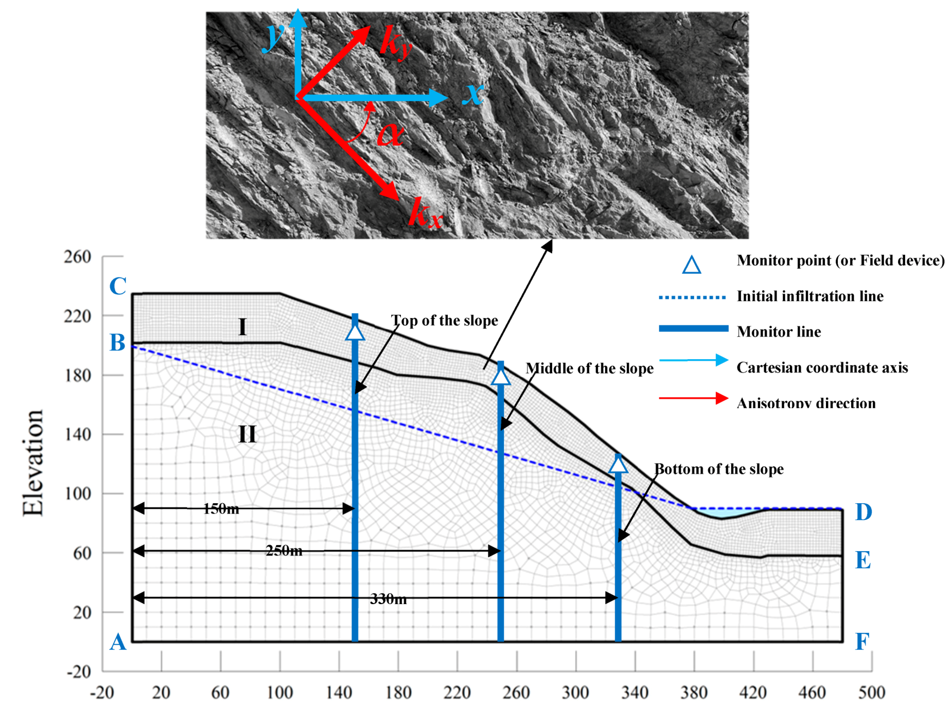
2.3. Finite Element Model and Boundary Conditions

The case study is a layered rock slope in the Pulang Region of Southwestern China, which is shown in Figure 1. In Figure 2, I and II represent strongly weathered carbonaceous slate and moderately weathered carbonaceous slate, respectively, which were characterized by bedding structures. This study’s finite element model of the slope body was 240 m high and 280 m long. The left and right borders extended horizontally for 50 m, and the lower border extended downward for 50 m, to eliminate any border effects. To investigate the strongly weathered layered slate, the grid size of the strongly weathered area was established as 2 m, and the grid size of the moderately weathered area was set as 10 m. The grid model was divided into 6333 nodes and 6208 elements, as shown in Figure 2. To study the characteristics of the seepage at different positions, three monitoring lines and three monitoring points were set at x = 150 m (top of the slope), x = 250 m (middle of the slope), and x = 330 m (bottom of the slope), and the monitoring points were located 10 m below the slope. In Figure 2, the boundary conditions are as follows: AB and FD are the fixed water level boundaries of 200 m and 90 m, respectively; CD indicates the boundary of the rainfall infiltration; BC and DE are the boundaries of small liquidity; AF is an impervious boundary. To restore the rainfall boundary, the average daily rainfall from 1 July to 1 August 2019 in the Pulang Region was adopted as the rainfall conditions, as detailed in Figure 3.

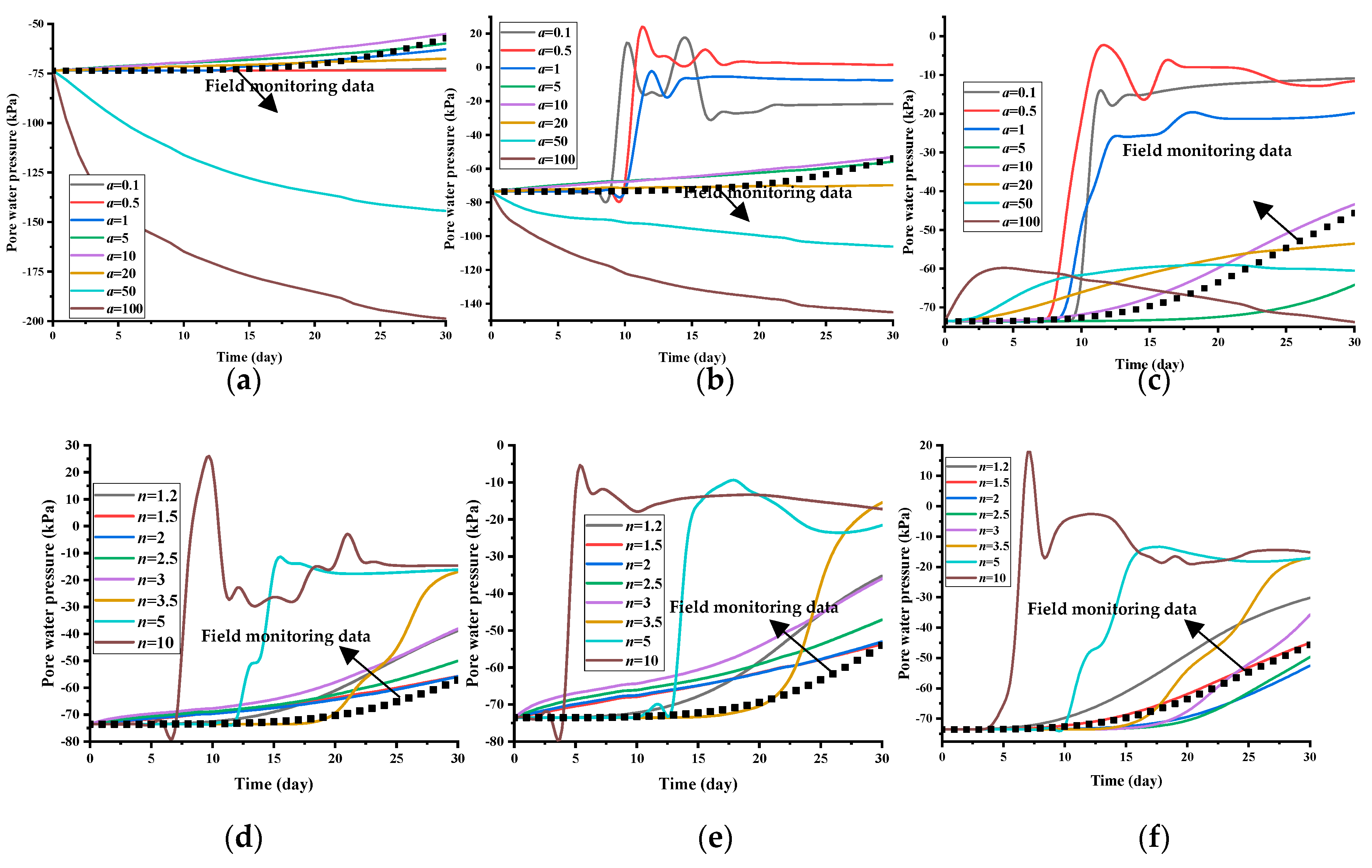
2.4. Determination of the Maximum Initial Matric Suction

Since the studied rock slope has a strong degree of weathering and the rock layers are so intensely fractured that the properties of soil or a porous medium can be assumed, it has a certain degree of matric suction. The extent of the initial maximum matric suction may vary, and the seepage states and stability levels of slopes may also be quite different. Therefore, to make the initial matric suction more in line with the actual situation (refer to previous studies [25,26]), this study set different maximum initial matric suctions as −50 kPa, −75 kPa, and −100 kPa, respectively, and the annual average rainfall of the Pulang area as 0.06 mm/h in the steady-state comparative analysis process. As detailed in Figure 4, the changes in the matric suction of the average annual rainfall were similar to the setting of the maximum initial matric suction of −75 kPa. Therefore, the initial maximum matric suction of all this study’s simulation experiments was set as −75 kPa, which was determined to be in line with the real situation in the study area.

2.5. Van Genuchten Model Parameter Sensitivity Analysis

Due to the difficulties encountered when measuring the unsaturated characteristic curves in rock masses, the water retention curves of classic unsaturated porous media [16,17,18,27] and relative hydraulic conduction models [19] are often used to describe the unsaturated flow in fissures and weakly permeable rock masses. Therefore, this study adopted the Van Genuchten Model to describe unsaturated features. The Van Genuchten Model is as follows [18]:

$$\theta ={\theta }_r+\frac{{\theta }_s-{\theta }_r}{{[1+{(p/a)}^n]}^m}$$

(3)

$$k=k_w\frac{{[1-{\left|p/a\right|}^{n-1}{(1+{\left|p/a\right|}^n)}^{-m}]}^2}{{(1+{\left|p/a\right|}^n)}^{\frac{m}{2}}}$$

(4)

where p is the suction, unit is kPa; θ indicates the adjusted volumetric water content, unit is m⁻¹; θ_r is the residual volumetric water content, unit is m⁻¹; θ_s indicates the saturated volumetric water content, unit is m⁻¹; a is the fitting parameter closely related to the air-entry value of the unsaturated rock mass, and the unit is kPa; n and m (m = 1 − 1/n and n > 1)are fitting parameters that control the slope at the inflection point in the volumetric water content function [18]. k_w is the saturated hydraulic conductivity, unit is m/s; k is the adjusted hydraulic conductivity, unit is m/s.

Parameters such as a, n, m, and θ_r are known to have major influences on the unsaturated flow of rock slope. For example, based on the analysis results of the seepage and stability of different slopes under the Fredlund and Xing parameters, Yu et al. [20] determined that the fitting parameters a, n, and m have major influences on the seepage characteristics of the slope. Additionally, Chen et al. [6] found that the unsaturated fitting parameters of the VG model were in the range of a = 0.2 to 100, m = 0.31 to 0.69, and n = 1.45 to 3.23 for rock masses. In a study by Jiang et al. [28], for general soil, the fitting parameters a = 100 and n = 2 were adopted in the Geostudio software, and for rock mass, the fitting parameter a = 10.

Therefore, this study referred to the recommendations of previous, related studies [6,18,20,28] and divided the parameters into three groups, as detailed in

Table 1. Calculation conditions.

Conditions	Fitting Parameter a (kPa)	Fitting Parameter n (m = 1 − 1/n)	Residual Volumetric Water Content θr (m−1)
Condition 1	10	[1.2, 1.5, 2, 2.5, 3, 3.5, 5, 10]	0.001
Condition 2	[0.1, 0.5, 1, 5, 10, 20, 50, 100]	1.5	0.001
Condition 3	10	1.5	[0.001, 0.005, 0.01, 0.02, 0.05]

. Since m = (1 − 1/n), this study chose to omit discussion of m.

In Figure 5a, parameter a represents the quantity closely related to the air-entry value of the unsaturated rock mass; the smaller the value of a, the more easily the water in the pores of the rock mass will be discharged. At the same time, due to the entry of air into the pores of the rock body, the water in the rock body will have difficulty flowing. Therefore, with decreases in the fitting parameter a, the hydraulic conductivity will drop earlier, which is shown in Figure 5d. As detailed in Figure 5b, the fitting parameter n controls the slope at the inflection point in the volumetric water content function. Therefore, with increases in parameter n, the slope part of the hydraulic conductivity of the rock will also increase, as shown in Figure 5e. It can be seen in Figure 5f that the residual volume of the water content has only a small effect on the hydraulic conductivity of rock. Therefore, θ_r can take any value from 0.001 to 0.05, so θ_r is set as 0.001 in this study.

Field monitoring data of pore water pressure were measured by the vibrating string type pore water pressure gauge (BGK10-BGK-4500S). The time and positions of field monitoring measurement are consistent with time and position the numerical simulation. It can be seen from Figure 6a,c that during the period of rainfall, the closer the fitting parameter a is to 10, the closer to field monitoring data the pore water pressure from the numerical simulation is. From Figure 6d,f, it can be seen that the closer the fitting parameter n is to 1.5, the closer to field monitoring data the pore water pressure from the numerical simulation is. So the fitting parameters of the water retention curve of the rock masses were determined, as detailed in

Table 2. Parameters of the water retention curve.

Layer	Materials	Fitting Parameters					Hydraulic Conduction Coefficient
		A (kPa)	m	n	θs	θr	k (m/s)
I	Strongly weathered carbonaceous slate	10	0.33	1.5	0.242	0.001	8.08 × 10−5
II	Moderately weathered carbonaceous slate	10	0.33	1.5	0.021	0.001	2.47 × 10−6

. Accordingly, the water retention curve of the rock mass is shown in Figure 7.

2.6. Definition of Anisotropy and the Calculation Conditions

It was found that the previous related studies had generally ignored the anisotropy ratio and angle. However, anisotropy widely exists in rock masses. In this study, the hydraulic conductivity matrix [C] was expressed as follows:

$$\left[C\right]=\left[\begin{array}{cc}{C}_{11}& C_{12}\\ C_{21}& C_{22}\end{array}\right]$$

(5)

In Equation (5), C₁₁ = k_xcos²α + k_ysin²α, C₂₂ = k_xsin²α + k_ycos²α, and C₁₂ = C₂₁ = k_xsinαcosα + k_ysinαcosα. The k_x and k_y, as well as the anisotropy angle α, were defined according to Figure 2. In the present study, k_x represents the horizontal hydraulic conductivity; k_y is the vertical hydraulic conductivity; α is the direction between k_x and x-axis. Therefore, if α = 0°, then [C] will be reduced to:

$$\left[C\right]=\left[\begin{array}{cc}{k}_x& 0\\ 0& k_y\end{array}\right]$$

(6)

Equation (6) was adopted in this study [29] with only the anisotropy ratio k_r = k_y/k_x considered. However, for the layered rock masses, due to the dip angles of the bedding plane, the conditions under which the anisotropy angle α is not equal to 0 should also be considered. Therefore, in this study, to restore a reasonable rock formation state, a dip angle range of between 50° and 70° in the layered rock slope in the Pulang area was taken into consideration. As shown in Figure 2, the anisotropic angle of hydraulic conductivity is equivalent to the dip angle of the layered rock slope. Combining the recommendations of previous related research [6,12,18,30,31,32], it was determined that the anisotropy ratio k_r was 0.01, 0.02, 0.1, and 1, and the anisotropy angle α was 50°, 55°, 60°, 65°, and 70°, respectively, neglecting the anisotropy of the moderately weathered carbonaceous slate, as detailed in

Table 3. Calculation conditions.

Rock Types	Anisotropy Ratio kr = ky/kx	Anisotropic Angle α (°)
Strongly weathered carbonaceous slate	$\left[\begin{array}{cccc}0.01& 0.02& 0.1& 1\end{array}\right]$	$\left[\begin{array}{ccccc}50& 55& 60& 65& 70\end{array}\right]$

. The failure criterion of the rock layered slope simulation adopted the Mohr-Coulomb Criterion, and the rock mass strength parameters were obtained from the geotechnical test results, as shown in

Table 4. Rock mass strength parameters.

Rock Types	Elastic Modulus (MPa)	Poisson Ratio	Unit Weight (kN/m3)	Cohesion (kPa)	Friction Angle (°)
Strongly weathered carbonaceous slate	2644.9	0.38	22.4	93.6	33.3
Moderately weathered carbonaceous slate	5561	0.35	26.5	120	35

.

3. Results and Discussion

3.1. Effects of The Hydraulic Conductivity Anisotropy on The Seepage Characteristics

3.1.1. Analysis of the Volumetric Water Content

According to the calculation conditions in Table 3, we carried out a total number of 20 numerical simulations, and obtained, in all, 60 sections of volumetric water content variation. The variations of the volumetric water content of different α values with k_r = 0.01 and k_r = 0.1 are shown in Figure 8 to illustrate the influence of anisotropy direction α on seepage characteristics, and different k_r values with α = 50° and α = 70° are also displayed in Figure 9 to show the impacts of anisotropy ratio k_r.

In Figure 8, the initial state was the distribution of the volumetric water content of the rock slope before rainfall, and the remainder was the distribution of the volumetric water content after the rain had ceased. Rainfall increased the volumetric water content of the surface of the rock slope, and the volumetric water content of the surface of the rock slope was affected by the anisotropy angle. Regarding the rock slope body, as the anisotropy angle decreased, the volumetric water content of the surface of the slope gradually increased. This was because a smaller the inclination in the plane led to a smaller hydraulic conductivity in the vertical direction, and a larger hydraulic conductivity in the horizontal direction, which prevented the rainwater from infiltrating into the deep part of the slope body and increased the surface volumetric water content of the rock slope.

Figure 9 shows that rainfall increased the volumetric water content of the slope, and that the volumetric water content of the slope was affected by anisotropy ratio k_r. It is worth mentioning that k_r had a great influence on the variation of water content in the shallow part of the bottom of the slope, as shown in Figure 9c,f. It can be seen in Figure 8 and Figure 9 that the turning point of the volumetric water content appeared within the shallow part of the rock slope. The moisture condition of the region above this point began to change from unsaturated to saturated, which indicated that the moist front had reached that turning point after the rain had ceased. The turning point of volumetric water content also appeared within the deep part of the rock slope. The moisture condition of the region above this point began to change from saturated to unsaturated, indicating that the groundwater line rose to this turning point after the rain had ceased.

3.1.2. Analysis of the Changes in the Groundwater Levels

As detailed in Figure 10a,c, the longer the duration of the rainfall event, the higher the groundwater levels rose. The increases in the groundwater level near the free face of the rock slope were found to be greater than those far from the free face. It is worth noting that when the rock masses were isotropic, the groundwater at the bottom of the slope decreased, since the hydraulic conductivity of the horizontal direction reached the maximum, and the horizontal drainage capacity the bottom of the slope was stronger than the vertical infiltration capacity of the rainwater, and the groundwater levels decreased. It can be seen in Figure 10d,e that when k_r was constant, it was found that with the increases of α, the differences in the heights of the groundwater levels near the free face of the rock were smaller. Then, when α was constant, with the anisotropy being increased, the differences in the heights of groundwater levels near the free face of the rock slope were larger.

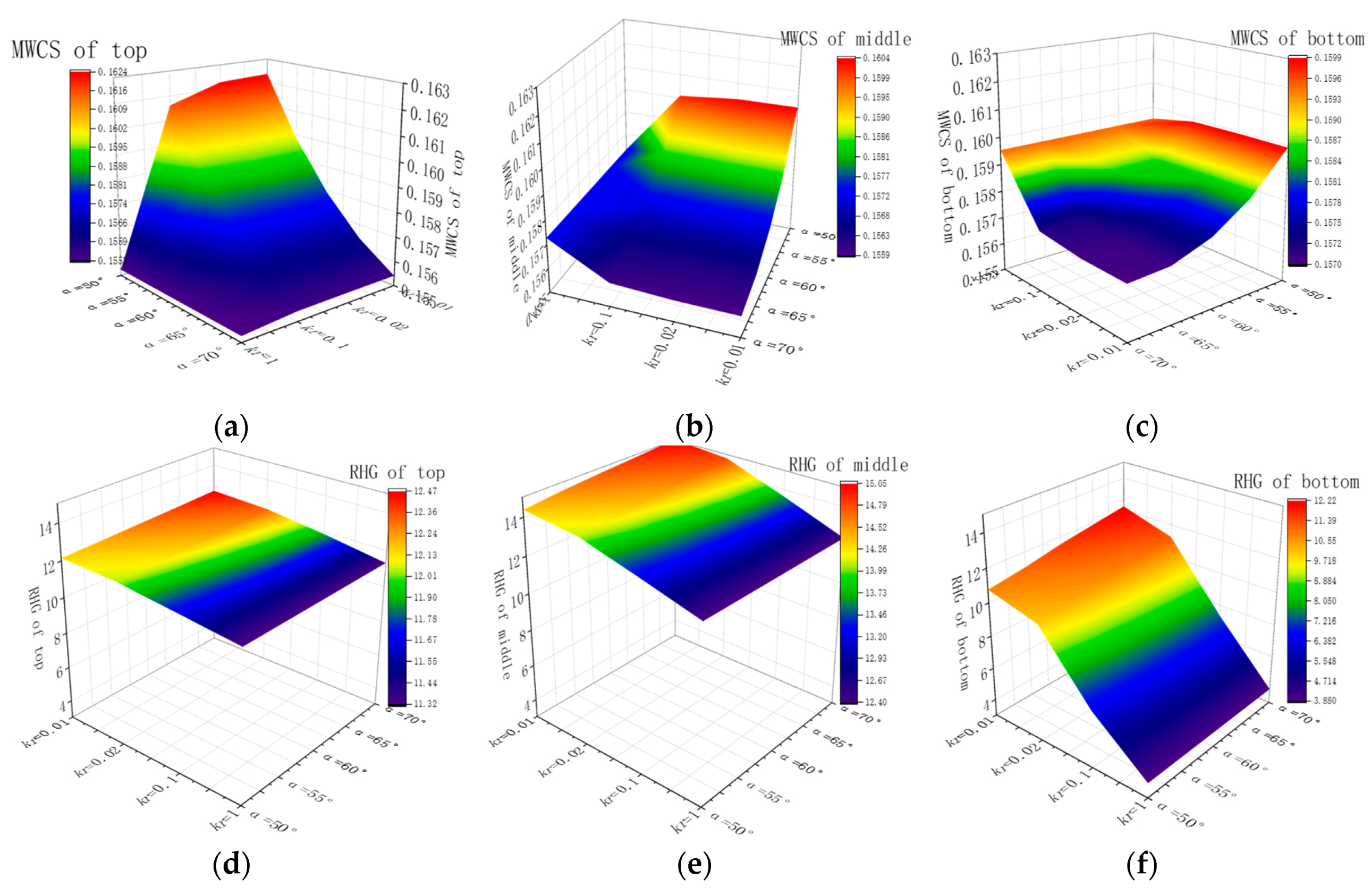
3.1.3. Analysis of the Maximum Water Content of the Surface and the Rising Height of the Groundwater

To more prominently examine the seepage characteristics of the rock slope under different k_r and α conditions, the maximum water content on the surface (MWCS) and the rising heights of the groundwater (RHG) were determined [25]. Figure 11 shows the variations of the volumetric water content on the slope over time. It can be seen in the figure that as the rainfall continued, the surface volumetric water content in the slope changed and gradually become saturated. Additionally, the maximum was reached at the end of the rainfall event. Therefore, the MWCS was used to describe the maximum water content on the slope surface during the rainfall event. As the rainfall infiltrated the slope, the groundwater level increased and the saturated areas expanded. Therefore, the RHG was used to describe the maximum height of the groundwater level increase when rainfall had subsided.

Figure 12 details the variations in the MWCS and RHG of the rock slope with different k_r and α. It can be seen in Figure 12a,c that MWCS increases gradually with the decrease of α. The reason for this is mentioned in Section 3.1.1. It is worth noting that with the change of k_r, MWCS has different change rules at different positions of slope body. At the top of the slope, MWCS gradually decreases with the increase of α. At the bottom of the slope, MWCS gradually increases with the increase of α. In the middle of the slope, the variations in α have little connection with MWCS under different k_r and α conditions. The variations of the MWCS at the top of the slope were found to range between 0.154 and 0.163 and the change rate was 5.8%. The variations of the MWCS at the middle of the slope ranged between 0.155 and 0.160, and the change rate was 3.2%. The variations of the MWCS at the middle of the slope ranged between 0.156–0.160, and the change rate was 2.6%, The maximum and minimum values of the MWCS both appeared at the top of the slope, and the change rate of the MWCS at the top of the slope was the largest, which indicated that the MWCS at the top was most greatly affected by the k_r and α. The change rate of the MWCS at the bottom of the slope was the smallest, indicating that the MWCS at the bottom was the least affected by the k_r and α.

It can be seen from Figure 12d,f that the RHG gradually increased with decreases in k_r and increases in α, since vertical penetration was enhanced and horizontal discharge was weakened, resulting in a large increase in the height of the water level. It was observed that under different k_r and α conditions, the variations of the RHG at the top of the slope ranged between 11.32 and 12.47 m and the change rate was 10.16%. The variations of the RHG in the middle of the slope ranged between 12.40 and 15.05 m and the change rate was 21.37%. Also, the variations of the RHG at the bottom of the slope ranged from 3.88 to 12.22 m and the change rate was 214.95%.

Therefore, it was found that the maximum value of the RHG appeared in the middle of the slope, and the minimum appeared at the bottom of the slope. The change rate of the RHG at the bottom of the slope was the largest, indicating that the RHG at the bottom was the most affected by the k_r and α. The RHG change rate at the top of the slope was observed to be the smallest, indicating that the RHG at the top was the least affected by the k_r and α.

3.2. Effects of the Hydraulic Conduction Anisotropy on the Stability of the Rock Slope

In the present study, the stability of rock slopes under different sliding surface conditions was comprehensively analyzed. Four arc sliding surfaces were assumed, referred to in this study as sliding surfaces 284, 293, 313, and 112, as shown in Figure 13. These types of sliding surfaces mainly penetrated through the strongly weathered layered slate. For the four types of surfaces, it was observed that as the rainfall continued, FS gradually decreased, as shown in Figure 14. It was found that under various anisotropy conditions, the differences in FS increased over time. When k_r = 1 (for example, when the rock layers were isotropic to seepage), the FS tended to be overestimated. When analyzing the stability of the layered rock slope, only the anisotropy of the shear strength was incomplete, and the anisotropy of seepage could not be ignored for the layered rock slope.

To complete a more in-depth examination of the stability of the different sliding surfaces of layered slopes under different k_r and α conditions, the FS after the rainfall had ceased were discussed. As detailed in Figure 15, it was observed that as the k_r decreased and the α increased, the FS of each sliding surface decreased. When k_r = 0.01 and α = 70°, the FS was found to be minimum. The FS of sliding surface No. 284 was determined to range between 1.41 and 1.47, and the rate of change was 4.26%. The FS of sliding surface No. 112 ranged between 1.49 and 1.60, and the rate of change was 7.38%. The FS of sliding surface No. 293 was observed to range from 1.57 to 1.67, and the rate of change was 6.37%. Additionally, the No. 293 sliding surface displayed a factor of safety of 1.66 to 1.70, with a rate of change of 2.41%. It was found that the smallest factor of safety occurred in the No. 284 sliding surface.

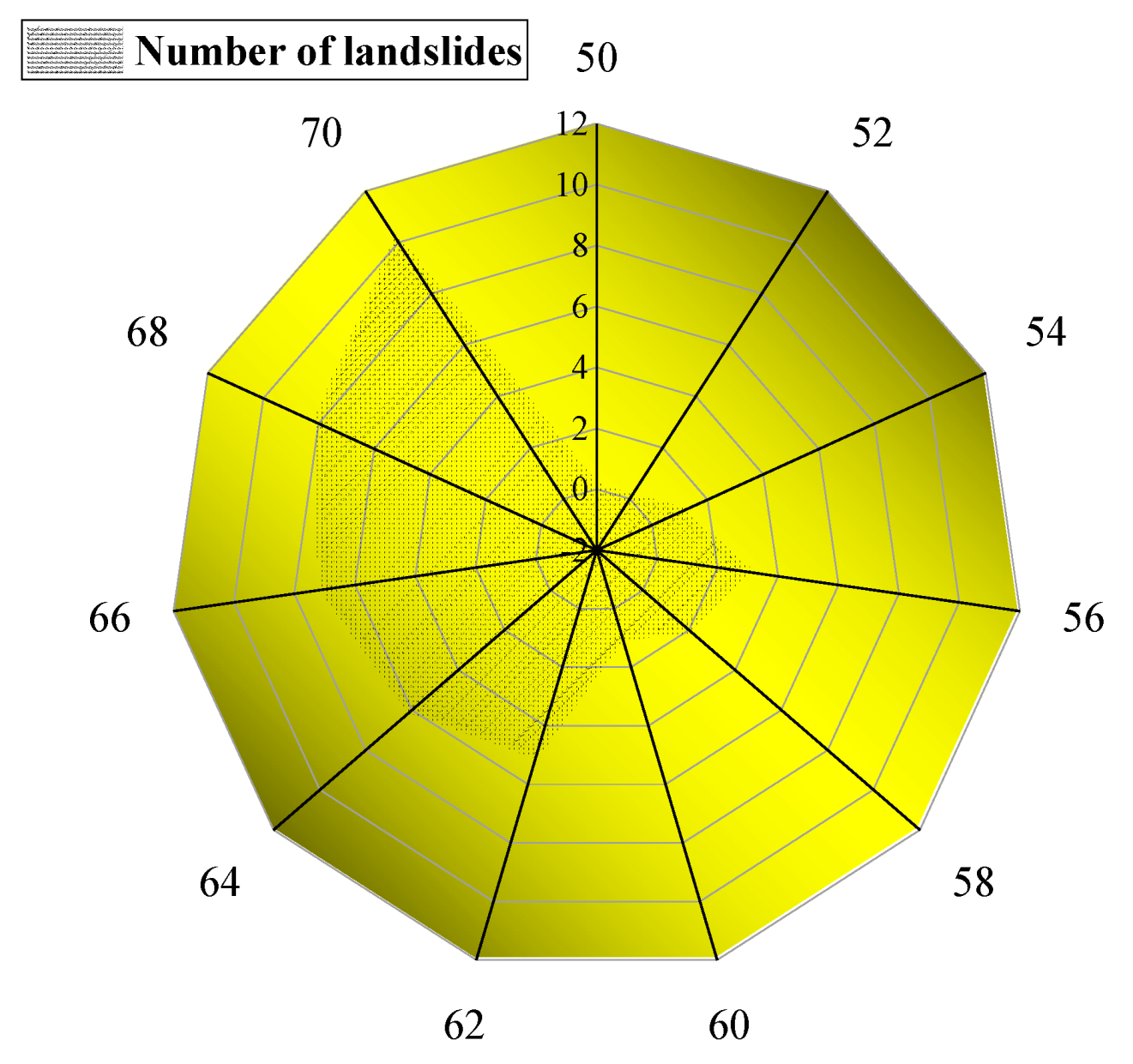
3.3. Field Investigation and Verification

Figure 16 shows some rock landslides in this area and their stereographic projections. It can be seen that most of the sliding surfaces of rock landslides are circular arcs in the strongly weathered layer, which verifies the assumptions regarding the arc sliding surface in Section 3.3. Although some stereographic projections show that the rocky slopes are stable, they still slip. It can be seen that they all present large dip angles. Figure 17 shows the results of the field survey of landslides in the Pulang region. The number of field landslides increases as the anisotropy angle increases, which verifies that as the dip angle of the bedding plane increases, the FS of rock slope decreases.

4. Conclusions

A layered rock slope in the Pulang Region, China was numerical simulated, considering different anisotropy ratios and anisotropy angles of hydraulic conductivity. Anisotropy ratios are the ratios of vertical hydraulic conductivity to horizontal hydraulic conductivity; anisotropy angles are the dip angles of the bedding plane. The research results were as follows:

(1)

The residual volumetric water content of the VG model had little effect on the hydraulic conductivity. The closer the fitting parameter a of the VG model was to 10, and the closer the fitting parameter n of the VG model was to 1.5, the closer the pore water pressure of the rock slope was to the field monitoring data.

(2)

The maximum initial matric suction was determined to be of major significance to the unsaturated seepage of the rock slope and the subsequent calculations. This study set the maximum initial matric suction to −75 kPa, which was determined to be consistent with the actual situation.

(3)

The different anisotropy ratios and dip angles of the bedding plane were found to have major impacts on the seepage in the layered rock slope.

(4)

The MWCS and RHG were determined to characterize the seepage characteristics of the rock slope. As the dip angles of the bedding plane decreased, the MWCS gradually increased. As the anisotropy ratios decreased and the dip angles increased, the RHG gradually increased.

(5)

When the seepage of layered rock slope was considered isotropic, the FS tended to be overestimated. As the anisotropy ratios decreased and the dip angles of the bedding plane increased, the FS of each sliding surface was reduced. When the dip angles of the bedding plane of the rock slope are larger, more essential protections are needed.

References

1. Zhang, Z.Y. Introduction to rock hydraulics. Geol. Hazards Environ. Prot. 1997, 6, 56. [Google Scholar]
2. Collins, B.D.; Znidarcic, D. Stability Analyses of Rainfall Induced Landslides. J. Geotech. Geoenviron. Eng. 2004, 130, 362–372. [Google Scholar] [CrossRef]
3. Dong, J.J.; Tzeng, J.H.; Wu, P.K.; Lin, M.L. Effects of anisotropic permeability on stabilization and pore water pressure distribution of poorly cemented stratified rock slopes. Int. J. Numer. Anal. Methods Geomech. 2006, 30, 1579–1600. [Google Scholar] [CrossRef]
4. Zbek, A.; Gül, M.; Karacan, E.; Alca, V. Anisotropy effect on strengths of metamorphic rocks. J. Rock Mech. Geotech. Eng. 2018, 10, 164–175. [Google Scholar]
5. Lee, C.L.; Shou, K.J.; Chen, S.S.; Zhou, W.C. Numerical analysis of tunneling in slates with anisotropic time-dependent behavior. Tunn. Undergr. Space Technol. 2019, 84, 281–294. [Google Scholar] [CrossRef]
6. Chen, Y.F.; Yu, H.; Ma, H.Z.; Li, X.; Hu, R.; Yang, Z. Inverse modeling of saturated-unsaturated flow in site-scale fractured rocks using the continuum approach: A case study at Baihetan dam site, Southwest China. J. Hydrol. 2020, 584, 124693. [Google Scholar] [CrossRef]
7. Yuan, J.P.; Lin, Y.L.; Peng, D.; Han, C.L. Influence of anisotropy induced by fissures on rainfall infiltration of slopes. Chin. J. Geotech. Eng. 2016, 38, 76–82. [Google Scholar]
8. Zhao, Y.L.; Wang, W.J.; Huang, Y.H.; Cao, P.; Wan, W. Coupling analysis of seepage-damage-fracture in fractured rock mass and engineering application. Chin. J. Geotech. Eng. 2010, 32, 24–32. [Google Scholar]
9. Gonzaga, G.G.; Leite, M.H.; Corthésy, R. Determination of anisotropic deformability parameters from a single standard rock specimen. Int. J. Rock Mech. Min. Sci. 2008, 45, 1420–1438. [Google Scholar] [CrossRef]
10. Yeh, P.T.; Lee, K.Z.Z.; Chang, K.T. 3D Effects of permeability and strength anisotropy on the stability of weakly cemented rock slopes subjected to rainfall infiltration. Eng. Geol. 2020, 266, 105459. [Google Scholar] [CrossRef]
11. Dong, J.J.; Tu, C.H.; Lee, W.R.; Jheng, Y.J. Effects of hydraulic conductivity/strength anisotropy on the stability of stratified, poorly cemented rock slopes. Comput. Geotech. 2012, 40, 147–159. [Google Scholar] [CrossRef]
12. Yu, S.; Ren, X.; Zhang, J.; Wang, H.; Wang, J.; Zhu, W. Seepage, Deformation, and Stability Analysis of Sandy and Clay Slopes with Different Permeability Anisotropy Characteristics Affected by Reservoir Water Level Fluctuations. Water 2020, 12, 201. [Google Scholar] [CrossRef] [Green Version]
13. Mandal, A.K.; Li, X.; Shrestha, R. Influence of Water Level Rise on the Bank of Reservoir on Slope Stability: A Case Study of Dagangshan Hydropower Project. Geotech. Geol. Eng. 2019, 37, 5187–5198. [Google Scholar] [CrossRef]
14. Illman, W.A.; Hughson, D.L. Stochastic simulations of steady-state unsaturated flow in a three-layer, heterogeneous, dual continuum model of fractured rock. J. Hydrol. 2005, 307, 37. [Google Scholar] [CrossRef]
15. Li, X.; Li, D. A numerical procedure for unsaturated seepage analysis in rock mass containing fracture networks and drainage holes. J. Hydrol. 2019, 574, 23–34. [Google Scholar] [CrossRef]
16. Brooks, R.H.; Corey, A.T. Hydraulic Properties of Porous Media; Colorado State University, Hydrology and Water Resources Program: Fort Collins, CO, USA, 1964; pp. 1–27. [Google Scholar]
17. Fredlund, D.G.; Xing, A. Equations for the soil-water characteristic curve. Can. Geotech. J. 1994, 31, 521–532. [Google Scholar] [CrossRef]
18. Genuchten, V.T.M. A Closed-form Equation for Predicting the Hydraulic Conductivity of Unsaturated Soils1. Soil Sci. Soc. Am. J. 1980, 44, 892–898. [Google Scholar] [CrossRef] [Green Version]
19. Mualem, Y. A new model for predicting the hydraulic conductivity of unsaturated porous media. Water Resour. Res. 1976, 12, 513–522. [Google Scholar] [CrossRef] [Green Version]
20. Yu, S.; Zhang, J.; Wang, J.; Wang, T.; Zhu, W.; Hu, N. Seepage and Slope Stability Analysis under Different Rainfall Patterns Based on Fredlund&Xing Parameters. J. China Three Gorges Univ. 2017, 39, 46–51. (In Chinese) [Google Scholar] [CrossRef]
21. GEO-SLOPE International Ltd. Seepage Modeling with SEEP/W 2007; Geo-Slope International Ltd.: Calgary, AB, Canada, 2010; pp. 1–207. [Google Scholar]
22. Morgenstern, N.R.; Price, V.E. The Analysis of the Stability of General Slip Surfaces. Géotechnique 1965, 15, 79–93. [Google Scholar] [CrossRef]
23. Johansson, J.M.A.; Edeskr, T. Effects of external water-level fluctuations on slope stability. Electron. J. Geotech. Eng. 2014, 19, 2437–2463. [Google Scholar]
24. Oo, H.Z.; Ai, L.; Qiu, Z. Numerical Analysis of River Bank Slope Stability During Rapid Drawdown of Water Level. Study Civ. Eng. Archit. 2013, 2, 98–103. [Google Scholar]
25. Yu, S.; Ren, X.; Zhang, J.; Wang, H.; Zhang, Z. Sensibility Analysis of the Hydraulic Conductivity Anisotropy on Seepage and Stability of Sandy and Clayey Slope. Water 2020, 12, 277. [Google Scholar] [CrossRef] [Green Version]
26. Tang, D.; Li, D.; Zhou, C. Slope stability analysis considering the antecedent rainfall process. Rock Soil Mech. 2013, 34, 3239–3248. [Google Scholar]
27. Fredlund, D.G.; Morgenstern, N.R.; Widger, R.A. The shear strength of unsaturated soils. Can. Geotech. J. 1978, 15, 313–321. [Google Scholar] [CrossRef]
28. Jiang, Z.; Xiong, X.; Zeng, L. Unsaturated seepage analysis of slope under rainfall condition based on FLAC3D. Geotech. Mech. 2014, 35, 855–861. (In Chinese) [Google Scholar] [CrossRef]
29. Yeh, H.F.; Tsai, Y.J. Analyzing the Effect of Soil Hydraulic Conductivity Anisotropy on Slope Stability Using a Coupled Hydromechanical Framework. Water 2018, 10, 905. [Google Scholar] [CrossRef] [Green Version]
30. Wang, Z.H.; Li, L.; Zhang, Y.X.; Zheng, S.S. Reinforcement model considering slip effect. Eng. Struc. 2019, 198, 109493. [Google Scholar] [CrossRef]
31. Zhang, Y.; Zhang, Z.; Xue, S.; Wang, R.; Xiao, M. Stability analysis of a typical landslide mass in the Three Gorges Reservoir under varying reservoir water levels. Environ. Earth Sci. 2020, 79, 42. [Google Scholar] [CrossRef]
32. Zhou, W.; Shi, X.; Lu, X.; Qi, C.; Luan, B.; Liu, F. The mechanical and microstructural properties of refuse mudstone-GGBS-red mud based geopolymer composites made with sand. Constr. Build. Mater. 2020, 253. [Google Scholar] [CrossRef]
Figure 1. Geographic location of the study area: (a) Study area location [6]; (b) Rock slope location.
Water 12 02314 g001
Figure 2. Grid model.
Water 12 02314 g002
Figure 3. Daily rainfall from 1 July to 1August 2019.
Water 12 02314 g003
Figure 4. Initial pore pressure distribution.
Water 12 02314 g004
Figure 5. Water retention curves and hydraulic conductivity curves: (a) Condition 1 of the water retention curve; (b) Condition 2 of the water retention curve; (c) Condition 3 of the water retention curve; (d) Condition 1 of the hydraulic conductivity curve; (e) Condition 2 of the hydraulic conductivity curve; (f) Condition 3 of the hydraulic conductivity curve.
Water 12 02314 g005
Figure 6. Variations in pore water pressure at the different positions under different a and n: (a) Top of the slope; (b) Middle of the slope; (c) Bottom of the slope; (d) Top of the slope; (e) Middle of the slope; (f) Bottom of the slope.
Water 12 02314 g006
Figure 7. (a) Water retention curve; (b) Hydraulic conductivity curve.
Water 12 02314 g007
Figure 8. Volumetric water content at different positions on the layered rock slope under different α values with kr = 0.01 and kr = 0.1: (a) Top of the slope with kr = 0.01; (b) Middle of the slope with kr = 0.01; (c) Bottom of the slope with kr = 0.01; (d) Top of the slope with kr = 0.1; (e) Middle of the slope with kr = 0.1; (f) Bottom of the slope with kr = 0.1.
Water 12 02314 g008
Figure 9. Volumetric water content levels at different positions on the layered rock slope under different kr values with α = 50° and α = 70°: (a) Top of the slope with α = 50°; (b) Middle of the slope with α = 50°; (c) Bottom of the slope with α = 50°(d) Top of the slope with α = 70°; (e) Middle of the slope with α = 70°; (f) Bottom of the slope with α = 70°.
Water 12 02314 g009
Figure 10. Variations in the groundwater levels: (a) kr = 0.01, α = 50° during rainfall; (b) kr = 0.01, α = 70° during rainfall; (c) kr = 1 during rainfall; (d) different α values with kr = 0.01 after rain had ceased; (e) different kr values with α = 70° after rain had ceased.
Water 12 02314 g010
Figure 11. Variations in the volumetric water content levels.
Water 12 02314 g011
Figure 12. Variations in the MWCS and RHG with different kr and α.: (a) MWCS of top of the slope; (b) MWCS of the middle of the slope; (c) MWCS of the bottom of the slope; (d) RHG of top of the slope; (e) RHG of middle of the slope; (f) RHG of the bottom of the slope.
Water 12 02314 g012
Figure 13. Locations of the sliding surfaces.
Water 12 02314 g013
Figure 14. Variations in the safety factors during rainfall: (a) 284 sliding surfaces; (b) 293 sliding surfaces; (c) 313 sliding surfaces; (d) 112 sliding surfaces.
Water 12 02314 g014
Figure 15. Variations in the safety factors of the different slip surfaces when rainfall ceased: (a) 284 slip surfaces; (b) 293 slip surfaces; (c) 313 slip surfaces; (d) 112 slip surfaces.
Water 12 02314 g015
Figure 16. Rock landslides and stereographic projections of rock slopes in the Pulang Region: (a) Landslide point No. 1; (b) Landslide point No. 2; (c) Landslide point No. 3; (d) Landslide point No. 4.
Water 12 02314 g016
Figure 17. Number of field landslides with different α (survey up to July 2019).
Water 12 02314 g017