1. Introduction
During the last few decades, infiltration basins and trenches have increasingly been used to spill water in the vadose zone with multiple purposes. First, they are a low-cost way to reclaim treated wastewater due to the natural filtering capacities of the unsaturated zone against organics, chemicals and contaminants. Moreover, in coastal areas affected by saltwater intrusion caused by overexploitation from pumping wells, this system may be a particularly efficient way to tackle contamination because the water infiltration acts as a barrier to saline encroachment and, at the same time, allows the recovery of salinized aquifers.
Described in the literature as groundwater replenishment, water-banking and artificial recharge, managed aquifer recharge (MAR) is the intentional recharge of water into aquifers for subsequent exploitation or environmental benefit. In the UNESCO Intergovernmental hydrological program (2014–2021), the specific role of MAR is to “improve security and quality of water supplies especially in water scarce areas under climate change and population growth”. The increasing number of study cases all over the world demonstrates that this approach represents a real opportunity for integrated water resources management in controlled conditions [
1].
In southeastern Iran, five floodwater-spreading systems for aquifer recharge, built between 1983 and 2001, decreased the water table drawdown and improved the groundwater quality [
2]. In Pakistan, leaky dams have been used to replenish depleting aquifers in the province of Balochistan [
3]. The leaky dam acts as a barrier, reducing the velocity of water runoff and retaining water, which increases rainwater movement into the aquifer. Borehole injections have been used in South Australia to store storm water runoff for peri-urban irrigation water supplies [
4]. In Spain, artificial recharge by irrigation channels is active in Southern Sierra Nevada [
5]; in Mexico this has been achieved through injection wells [
6] and in Hungary using bank filtration [
7]. In Portugal and Palestine, different strategies for MAR were applied with the support of a DSS in order to evaluate the robustness of identified MAR sites [
8].
These cases demonstrate that, under controlled conditions, this approach represents an effective solution for the integrated water resources management as part of wider water management strategies [
9].
Although the application of MAR, often associated with Soil Aquifer Treatment (SAT), is subjected to severe restrictions in terms of water quality, water percolation through infiltration basins has become a useful way to store or recover water in the subsurface [
10]. Regardless of the purpose of their use, an accurate knowledge of the geology and hydrogeology of the filtering medium is required, in both the planning and operational stages of the infiltration trenches, in order to better understand the hydrological response of the system and its efficiency over time. Particularly in the case of MAR or SAT plants involving surface spreading systems, it is crucial to accurately estimate how fast the infiltrated water moves in the subsoil so as to assess the filtering capability of the unsaturated medium in different saturation conditions and its maximum water storage capability.
Unfortunately, the infiltration capacity is not constant during the life cycle of a trench. Surface water or treated wastewater, generally used for artificial recharge, can contain significant quantities of sediments, suspended particles and microorganisms, which lead to clogging of micropores, fissures and fractures. This phenomenon has multiple effects, including the reduction of the infiltration rate, the necessity of regular maintenance (e.g., scraping of the basin floor or the replacement of the filter bed), and, in extreme cases, site abandonment [
11]. Clogging can be caused by different processes: physical (deposition of organic and inorganic solids carried in suspension), biologic (accumulation of microbial cells and their metabolic byproducts), chemical (precipitation of minerals from water) and gas bubble formation (entrapped air and biogenic gases) processes. Each of these processes can occur individually or together. The development and extent of clogging are influenced by different factors including the quality of the spread water, bedrock type, ponding depth, hydraulic loading rate and cycle and presence of vegetation. As all of these factors change over time, the clogging processes can be variable [
12,
13]. This makes the detailed understanding of clogging effects a great challenge.
This issue is even more critical in fractured and karstic systems, where the strong heterogeneity causes high variability in flow and transport processes in terms of both direction and rate. In fact, compact rocks with very low hydraulic conductivity are locally affected by fractures or karstic forms that represent significant preferential flow pathways. In these complex unsaturated systems, field hydraulic properties, typically water content and hydraulic conductivity, are very difficult to estimate with the standard measurement procedures suitable for unconsolidated material, and very few examples of measurements on rocks are documented to date. The main difficulty regards the insertion of the sensors, which need to be hammered or require drilling into the rock, often causing brittle fractures. Furthermore, it is very difficult to ensure good contact between the rock and the sensors, a necessary precondition to avoid significant errors in the investigated properties [
14,
15].
Numerous predictive numeric models have been developed to describe clogging in porous or fractured media in the laboratory or in field tests [
16,
17]. However, accurate and spatially distributed hydrological constraints based on a priori geological observations are needed to take into account the very small scale of the representative elementary volume (REV) needed [
18].
In light of these considerations, optimal management of the infiltration trenches requires a detailed and cost-effective monitoring of infiltration processes at increasing depths below the infiltration trenches. Classical hydrological observations such as water ponding heads at the trench bottom are conventionally measured to provide estimations of the infiltration rate and hydraulic conductivity. However, these are overall measurements and provide limited details on how water infiltrates in the saturated–unsaturated subsurface.
For this reason, such measurements are increasingly combined with noninvasive geophysical techniques, able to image subsurface structures and rock–water interaction with high spatial resolution through physical parameters strictly related to the hydrological ones. In the last few decades, the use of electrical techniques to monitor infiltration dynamics became widespread due to the high sensitivity of the electrical resistivity to the water movement [
19,
20,
21,
22,
23,
24,
25,
26]. Particularly in the context of SAT and MAR applications, several study cases concerned time-lapse ERT monitoring [
27,
28,
29,
30,
31,
32] to investigate the sensitivity of the methods to changes in subsurface properties, to highlight the spatiotemporal distribution of the infiltrated water and improve the design and operation of MAR systems.
In this study, we propose a combined hydrogeophysical approach based on water level observations and geophysical monitoring at the experimental site of Castellana Grotte (Bari, Italy), where, since 2016, around 2300 m3d−1 of tertiary wastewater treatment effluent has been alternatively poured in nine infiltration trenches by adopting an almost daily recharge cycling. The combined approach was applied to monitor wastewater infiltration dynamics in two different periods, corresponding to the maximum and minimum rainfall of the wet and dry season, respectively.
In particular, the monitoring of water levels was matched with time-lapse electrical resistivity tomography (ERT) to assess the impact of the wetting–drying cycles in the vadose zone. The aim was to visualize the infiltration pattern variations, over space and time, in the upper portion of the fractured vadose zone, which mainly influences the water infiltration and the life cycle of trenches. For this purpose, changes in saturation degree were estimated during the infiltration process, with this parameter being particularly suitable for capturing the hydrological response of fractured and karstified rock systems.
2. Site Description
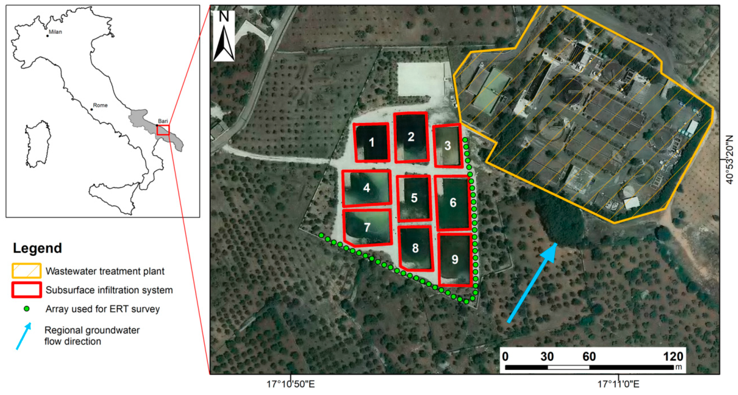
The experimental site is close to the urban wastewater treatment plant of the municipality of Castellana Grotte, 45 km SE of Bari (Southern Italy) (
Figure 1) and is adopted as final receptor of the treatment plant effluents. The system has been fully operational since 2016, with 2300 m
3d
−1 of treated water spread in the trenches on a rotating basis about every 2–3 days.
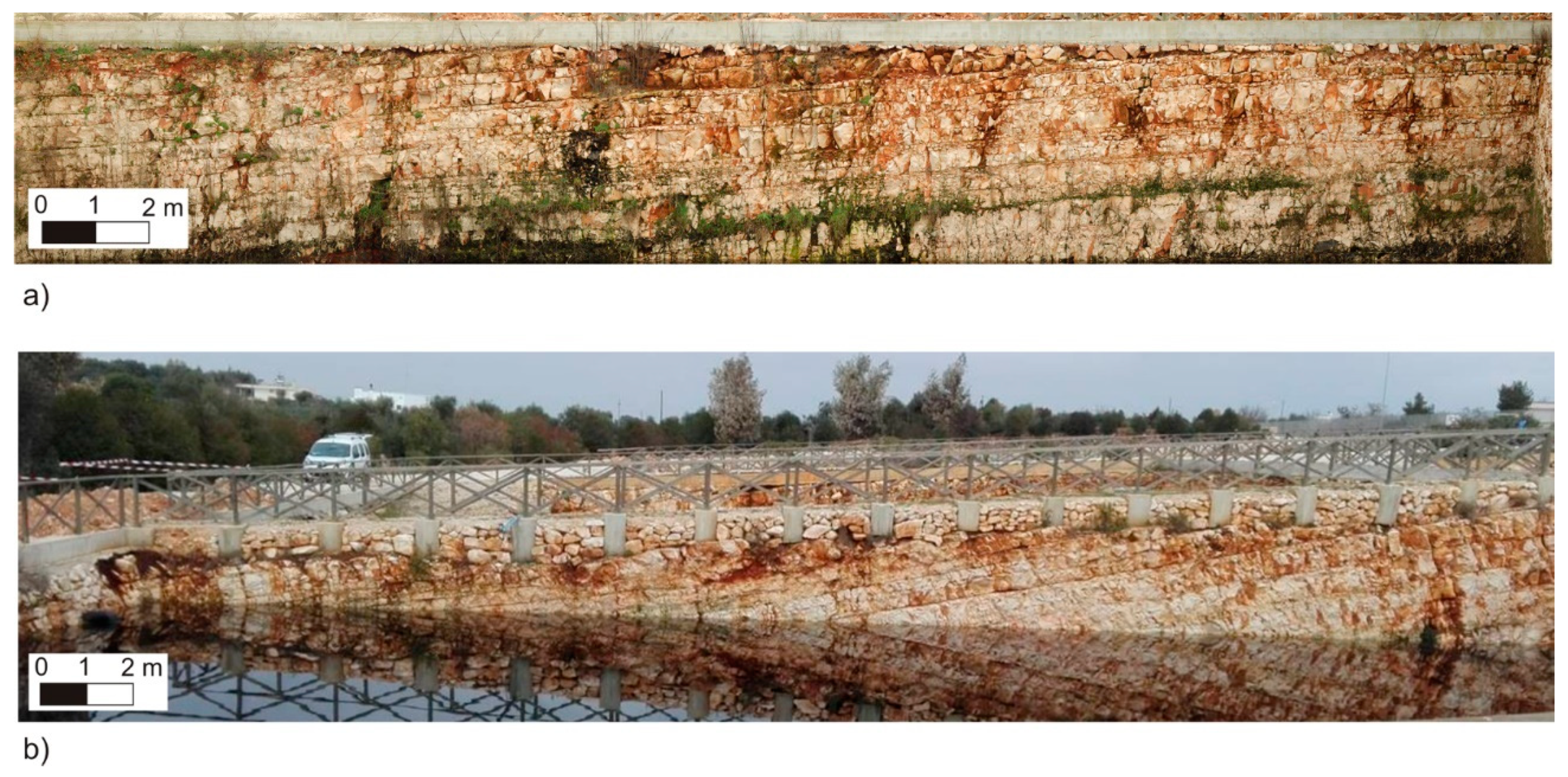
The nine trenches are arranged on slightly north-sloping ground and have a rectangular shape (average dimensions: 20 m × 30 m), with the major alignment oriented N–S and vertical walls with depths ranging from 3 to 5 m. A thin gravel layer overlays the bottom of each trench as a filtering media for the poured water. From a geological point of view, the unsaturated zone hosting the trenches is made up of stratified limestone, dolomitic limestone and dolomites belonging to the Calcare di Altamura Formation (Upper Cretaceous). The carbonate sequence is often faulted, intensively fractured and affected by karst dissolution phenomena. The huge complex of karst caves (known as the Castellana Caves), located 3 km SW of the plant, is evidence of the phenomenon.
A typical feature of this karstic environment is the epikarst, a zone located at the top of the vadose zone (with thickness between a few meters and a few tens of meters) with a marked anisotropy in the stratigraphic layout (
Figure 2). The infiltration water percolates downward, flowing from the epikarst through a vadose zone to reach the saturated zone. In the study area, a thick unsaturated transmission zone overlays the water table, located more than 240 m below the surface level. Adopting a Darcy model, with unit–gradient hypothesis for the infiltration through the lateral and bottom surfaces, the horizontal and vertical hydraulic conductivity were calibrated after some infiltration tests undertaken in March 2017, thus obtaining 1.66 × 10
−5 ms
−1 and 5.00 × 10
−6 ms
−1, respectively.
The horizontal-to-vertical hydraulic conductivity ratio value is consistent with other experimental values observed in fractured and karstified systems, widely reported in the scientific literature [
33,
34].
The treatment plant, managed by regional water utility Acquedotto Pugliese (AQP S.p.A.), collects wastewater coming from the main urban area and some small suburbs around the plant, accounting for 20,000 inhabitants in total. The wastewater is treated to a high standard of water quality, as confirmed by the gross parameters summarized in
Table 1.
Through a network of pipelines, the treated wastewater is spread into a subsurface infiltration system consisting of nine trenches with a total surface of 9000 m2. This study focuses on Trench 9, located upstream with respect to the other trenches, which is one of the best performing and therefore most used.
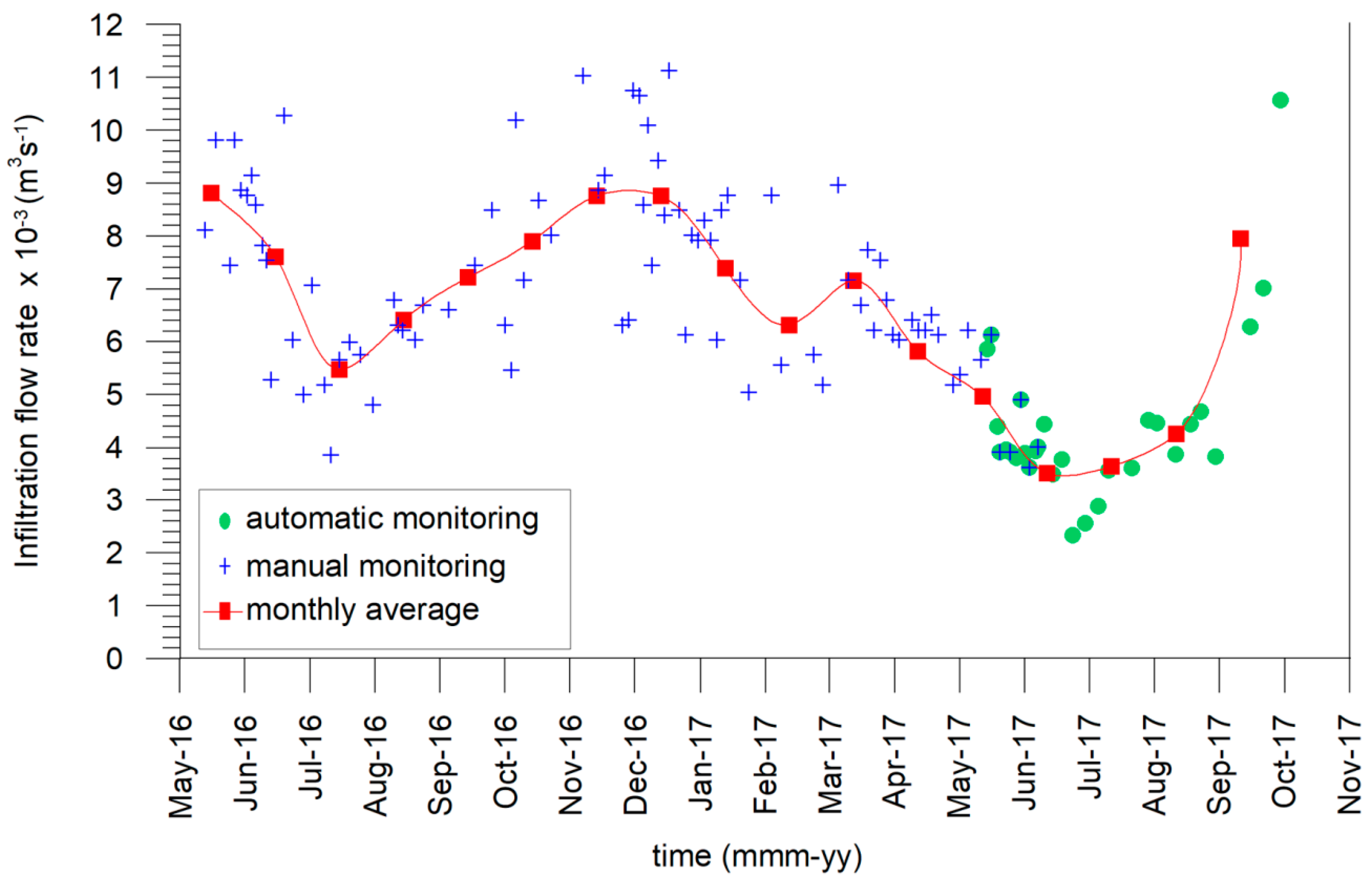
Seasonal changes in the infiltration flow rate were observed through water level data available since May 2016. By selecting the descending sections of the water level curve only, between 1.8 and 0.4 m, a trench-averaged infiltration flow rate was calculated for each descending section using the drawdown of water level in the trench per unit of time and its surface area.
Figure 3 shows the calculated infiltration flow rates and the monthly averages.
The seasonal variation in infiltration rate is highlighted in
Figure 3, with smaller values recorded in the summer period (June–September). Moreover, comparing the two summer periods (2016–2017), a decrease of the trench infiltration capacity is observed, although the short time series does not allow for extrapolating significant trends.
For this reason, the hydrogeophysical monitoring focused on a narrower temporal window in order to investigate the main features of the infiltration dynamics over the study period.
3. Materials and Methods
3.1. Field Experimental Setup: Water Level Monitoring
Since March 2017, the water level and temperature were continuously monitored in the infiltration trenches to estimate their drainage efficiency over time. For this experiment, infiltration Trench 9, located upstream of the others, was chosen in order to avoid overlapping effects due to the interference among the adjacent trenches. In fact, water flow can occur through the walls (septa) that separate the trenches from each other, due to the small thickness of the septa, ranging from 3 to 5 m and the presence of fractures and karstic forms in the hosting rocks. The infiltration trench—35 m long, 25 m wide, and 5 m deep—was equipped with a multiparametric probe (CTD-DIVER, Eijkelkamp, The Netherlands), installed close to the bottom, that records water level, temperature and electrical conductivity measurements every 10 min. The probe was installed at the north side of the trench, corresponding to the outlet of the treated wastewater into the trench.
In order to better evaluate the variations in the infiltration process within the epikarst under different wetting conditions of the rock profile, two monitoring periods were chosen: March 2017, roughly corresponding to the end of the maximum rainfall period (wet season); and July 2017, corresponding to the minimum rainfall period (dry season).
During these periods, two different spreading modes were adopted to pour water into the trenches. In March, the switch of the water spilling among the trenches was operated manually, while in July it was operated automatically upon reaching a threshold value of the water level in the trench. These modes led to a different trend in the wetting and drying cycles. In fact, in a week of observations three cycles were recorded in March, while a single cycle was recorded in July.
3.2. Basics of Electrical Resistivity Tomography
The electrical resistivity tomography (ERT) technique was used to image infiltration dynamics due to its high sensitivity to water content [
35].
The rock electrical resistivity or its inverse electrical conductivity, mainly depends on fluid flow into the medium through micropores and fractures. Among the several petrophysical models commonly used, Archie’s law [
36] defines an empirical correlation between the rock electrical resistivity to porosity and saturation degree or water content:
where
ρ is the rock resistivity, expressed in Ω m,
ρw is the resistivity of the fluid in the pore space, ϕ is the porosity, S
w is the saturation degree and m and n are Archie’s parameters that are calibrated in the laboratory. When rock resistivity increases, the saturation degree or water content decreases and vice versa. The use of Archie’s law expressed in Equation (1) is valid only for sedimentary rocks that are clay-free; otherwise, additional surface conductivity cannot be neglected [
37]. In fractured carbonate rocks, the contribution of the surface conductivity could be provided by the filling material, typically named “terra rossa”, i.e., a carbonate rock residue mainly made of oxides and hydroxides of iron and aluminum, illite and kaolinite, which occlude fissures and fractures in the rock matrix.
Furthermore, the term
ρw must be assumed to be constant over space and time in order to exactly correlate the variation in saturation degree to changes in bulk electrical resistivity [
38] and to avoid dual domain effects [
39].
On the other hand, in fractured and karstic systems, fracture density and length distributions impact the effective electrical properties of rocks.
Particularly in low-porosity fracture–matrix systems, simplified fracture network models, such as Archie’s law, are not representative of realistic field conditions and may not be adequate to model the electrical properties of the medium; on the contrary, high fracture densities lead to simplified behaviors that can be described with Archie’s law [
40].
However, in fractured rock systems, electrical techniques are a powerful tool to detect preferential pathways [
41,
42] and provide estimations of the main rock parameters, such as secondary porosity, dip and strike angle [
43].
An ERT survey was carried out by placing the electrodes on the ground surface around the trench, using an L-shaped geometric array due to the practical difficulties to install sensors at the bottom of the trench without affecting the geophysical data. This unconventional array is particularly useful when it is not possible to install the electrodes above the target to be detected. Therefore, 48 stainless-steel electrodes, with 5 m between each one, were permanently installed along two sides of the selected trench for the entire monitoring period (
Figure 1) in order to collect apparent resistivity data, which refer to a homogeneous subsurface resistivity model. From the apparent data, a resistivity model is achieved through an iterative inversion procedure
3.2.1. Sensitivity Analysis and Forward-Modeling
In the case study, two main critical points were faced during the planning of the ERT survey: (1) the sensitivity of the unconventional L-shaped electrodes’ configuration array to detect features below the bottom of the trench with high geophysical resolution and (2) the impact of the variable water head during the wetting–drying cycles on the flow current in the subsurface and hence on the resistivity modeling. In order to minimize these model uncertainties and simulate different saturation degree conditions in the subsurface, several forward simulation models were developed using different resistivity perturbations, and sensitivity maps were generated for each simulation setup.
Forward-modeling and sensitivity analysis play a critical role in predicting the geophysical response in complex areas in order to plan the optimal survey design in terms of geometry and data acquisition parameters.
The spatial sensitivity distribution is a property of the array that does not change with the perturbation properties [
44], allowing us to define the depth of investigation, while forward-modeling depends on ERT survey design and model parametrization [
45].
Several synthetic models were built to simulate the system response in order to address such critical issues. Particularly to assess the effect of the variable hydraulic head within the trench on the subsurface resistivity distribution, two synthetic models were generated with hydraulic heads equal to 0.60 m and 2.70 m, respectively, corresponding to about the minimum and the maximum hydraulic head recorded in the trench. The water resistivity was set to 10 Ω m, the above quasi-infinitive air resistivity to 100,000 Ω m and the subsurface resistivity to 1000 Ω m.
Other synthetic models were built to evaluate the ability of the ERT design to predict resistivity changes below the trench during the drying–wetting process.
A 10-m-thick layer between −5 m and −15 m below ground surface (bgs) was perturbed, with resistivity values ranging from 100 to 800 Ω m, in order to simulate the response of the system in terms of water content variations. The subsurface resistivity was set to 1000 Ω m and the mean hydraulic head recorded during the drying–wetting cycles was set to 1.20 m for both cases.
For each synthetic ERT dataset, a combination of 2212 Wenner–Schlumberger resistance measurements with skip 0 (minimal distance between potential electrodes equal to one electrode spacing) was generated using the same geometry as in the field experiment.
A grid size of a tetrahedral structured finite element mesh was set equal to 1.5 m in all directions with a total number of mesh nodes equal to 50,592 and 46,530 blocks. In order to match the field case, the synthetic inversion parametrization was the same as the field data inversion [
46].
ERTLAB forward solver tool was used to calculate the synthetic resistance data for each ERT-snapshot data.
The generated synthetic data were inverted to estimate the 3D electrical resistivity field using ERTLAB commercial software (MultiPhase Technologies, LLC, Sparks, NV, USA in collaboration with GeoStudi Astier SRL, Livorno [LI], Italy), based on a smoothness-constrained Occam’s inversion scheme.
In order to provide a realistic test of the inversion, 5% random noise was added to the data.
A robust inversion scheme, based on data variance iterative reweighting, was used to appropriately manage the effect of non-Gaussian noise [
45].
3.2.2. Time-Lapse ERT Monitoring
The time-lapse ERT surveys were carried out in March and July 2017, corresponding to the peak of the wet and dry season, respectively.
Syscal Switch Pro 48 (Iris Instruments, Orleans, France) was used to collect time-lapse resistivity measurements. In order to ensure good-quality data, the stacking (repetition of acquisitions within a cycle of measurement) was set from 3 to 6 and the maximum standard deviation was fixed to 5%. Moreover, the injection pulse length was set to 250 ms. Acquisition of each dataset took about 7 min.
The geophysical monitoring period covered about six days. More than 40 acquisition cycles were collected for each seasonal monitoring period. The resistivity data were recorded every 3 h and conveyed in remote mode using Comsys Pro code (Iris Instruments, Orleans, France).
Due to the potential noise, close attention was devoted to the data processing and inversion procedure.
In order to correctly invert the whole dataset, in the preprocessing step the bad raw data were normalized with respect to the temperature [
47] and filtered out by removing anomalous spikes of injected current, measured potential, and the data exceeding the threshold value of 5% in standard deviation.
After the filtering process, the resistivity data decreased from 2212 to 1643 data points for each dataset, and the total number of measurements considered for the inversion was about 60,000.
An approach based on the inversion of the resistance ratios measured at different time points with respect to the background was adopted to enhance time-lapse resistivity changes [
19]. This approach was widely used to track small variations in resistivity over time [
48,
49,
50,
51,
52]. It is particularly suited to electrically noisy sites because the modeling errors and data errors correlated over different time steps are minimized, and imaging artifacts that typically would occur in a standard inversion are avoided.
For each quadrupole, the resistance ratio R, expressed in Ohm, was recalculated using Equation (2):
where R
t is the resistance measured at time t; R
0 is the background resistance measured before starting the infiltration tests and R
ohm is the resistance for a homogeneous medium chosen to have a uniform resistivity equal to 100 Ω m, calculated by averaging the whole set of apparent resistivity ratios.
Moreover, this approach allowed for using a simplified Archie’s law that provides a hydrological meaning to the geophysical findings by directly converting the resistivity ratio into changes in saturation degree.
The simplified Archie’s law was written in the form:
where the resistivity ratio was provided by the inversion procedure and the term “n” was calibrated by laboratory measurements and set equal to 2.
In the specific study case, Archie’s model was suited to describe the electrical properties of the fractured rock for three main reasons: (1) the contribution of the surface conductivity was assumed to be negligible because of the cyclic drying–wetting phases, which have been occurring since the start of plant operation in 2016, and should have washed out the clayey filling in the fractures; (2) the fracture density estimated on the excavation walls of the trench is about 10, which is above the percolation threshold defined in [
40]; (3) the fluid electrical conductivity σ
w did not change over time because, during the monitoring, the water circulating in the rock formation is solely the treated wastewater that percolates through the trenches. In addition, in the two temporal windows considered for the ERT monitoring the electrical conductivity of infiltrated water was steady around 1.020 mS cm
−1, making dual domain effects negligible to the overall conductivity.
3.3. Infiltration Efficiency
The metric of infiltration efficiency was introduced in [
53] as an alternative to the infiltration rate for monitoring recharge. This was defined as the infiltration rate divided by the maximum possible infiltration rate. At a local scale, this parameter indicates the percent of the maximum infiltration rate achieved at a specific location and time, allowing for the identification of clogging effects.
Using well-known correlations that relate the hydrological, thermal and electrical properties of the filtering medium, the local infiltration efficiency can be estimated through different sensors located on the bottom of the trench, such as a distributed temperature sensor (DTS) or electrical conductivity sensors, as exhaustively discussed in [
53].
This metric was used to highlight how soil heterogeneity affects clogging processes, which, in turn, can significantly impact the performance of MAR operations [
54].
In this case study, the local infiltration efficiency was estimated in March through time-lapse geophysical data in order to enhance the different infiltration patterns due to rock heterogeneity.
It was derived in two specific points, the centroids of the south and north portions of the trench, at a depth of −5 m bgs using the following equation:
where q(
t) and σ(
t) are the infiltration rate and the electrical conductivity at time t, respectively; q
max and σ(
t0) are the maximum infiltration rate and the maximum electrical conductivity measured during the infiltration period at the same location, respectively; and β is the exponent of a power law relationship between hydraulic and electrical conductivity.
While the electrical conductivities are provided as the inverse of the electrical resistivity, it is very difficult to estimate the value of β in fractured and karstic rock, because an accurate value of this parameter would require a large number of core samples, given the high heterogeneity of the medium. For convenience, a value of 2 was set, but an overestimation or an underestimation cannot change the pattern of the local infiltration efficiency over time.
4. Results
4.1. Water Level Monitoring
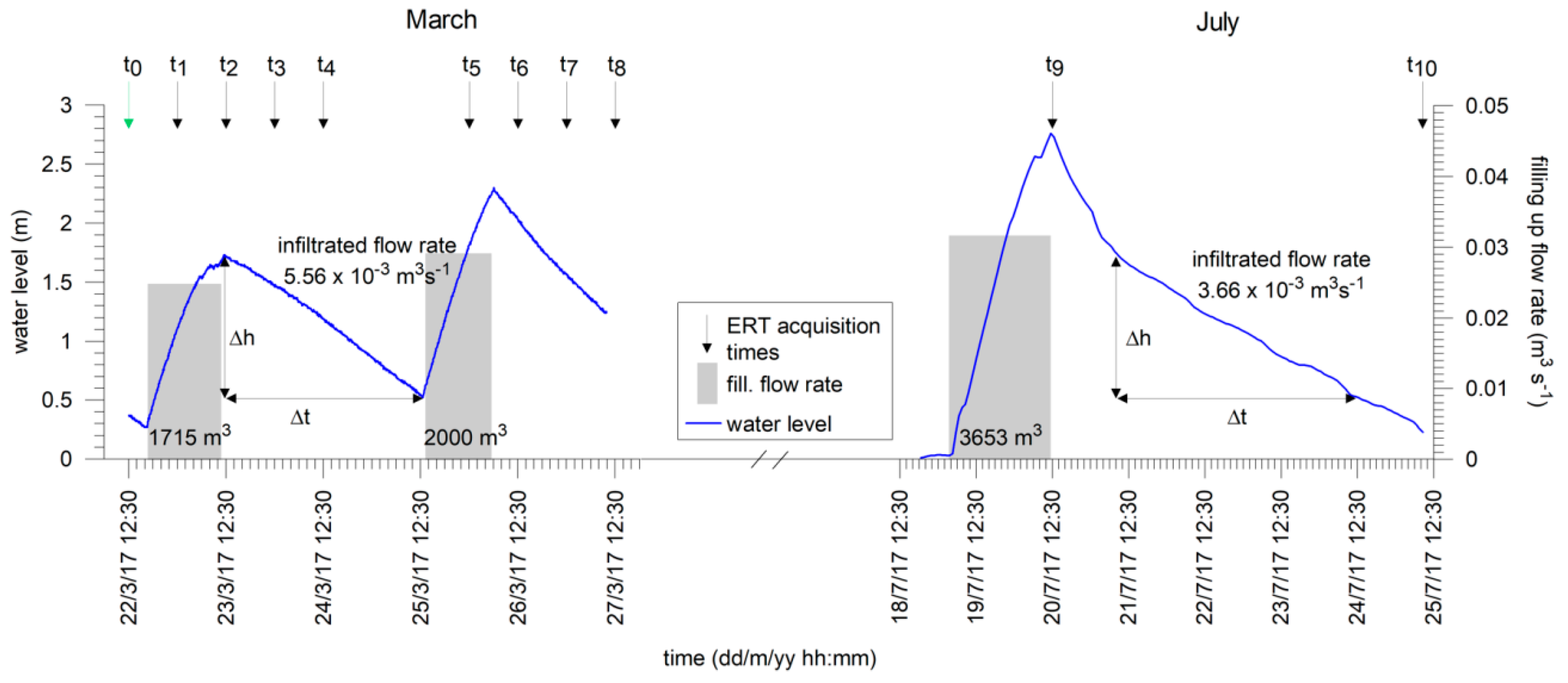
Figure 4 shows the fluctuations of the water level recorded in the Trench 9 and the filling-up flow rates during the March and July tests. The bottom of the trench was considered as a reference for water level measurements. The trend, correlated with the different spread modes in the two observation periods, is clearly highlighted.
In March, the manual operation of the water spread in the trench led to a double spread, which means a higher frequency of the trench water level increase–decrease cycles and to lower absolute hydraulic head values (1.73 and 2.27 m). In these cycles the filling-up volumes were 1715 m3 and 2000 m3, respectively.
Conversely, in July a higher absolute hydraulic head (2.76 m) was reached with a single filling-up phase, for a total volume of 3653 m3.
An observation period corresponding to the time during which the water level declined from 1.70 m to 0.55 m was considered in order to reliably compare the datasets collected in the two monitoring campaigns.
Two different slopes were highlighted in the recession hydrographs, reflecting a higher infiltration flow rate in March (5.56 × 10⁻³ ms−1) with respect to that recorded in July (3.66 × 10⁻³ ms−1) for the reference period.
The different trends between the two periods could be explained by the presence of a thin biofilm layer observed on the trench walls, with persistent algal blooms on the water surface during the warm season.
4.2. Forward-Modeling and Sensitivity Results
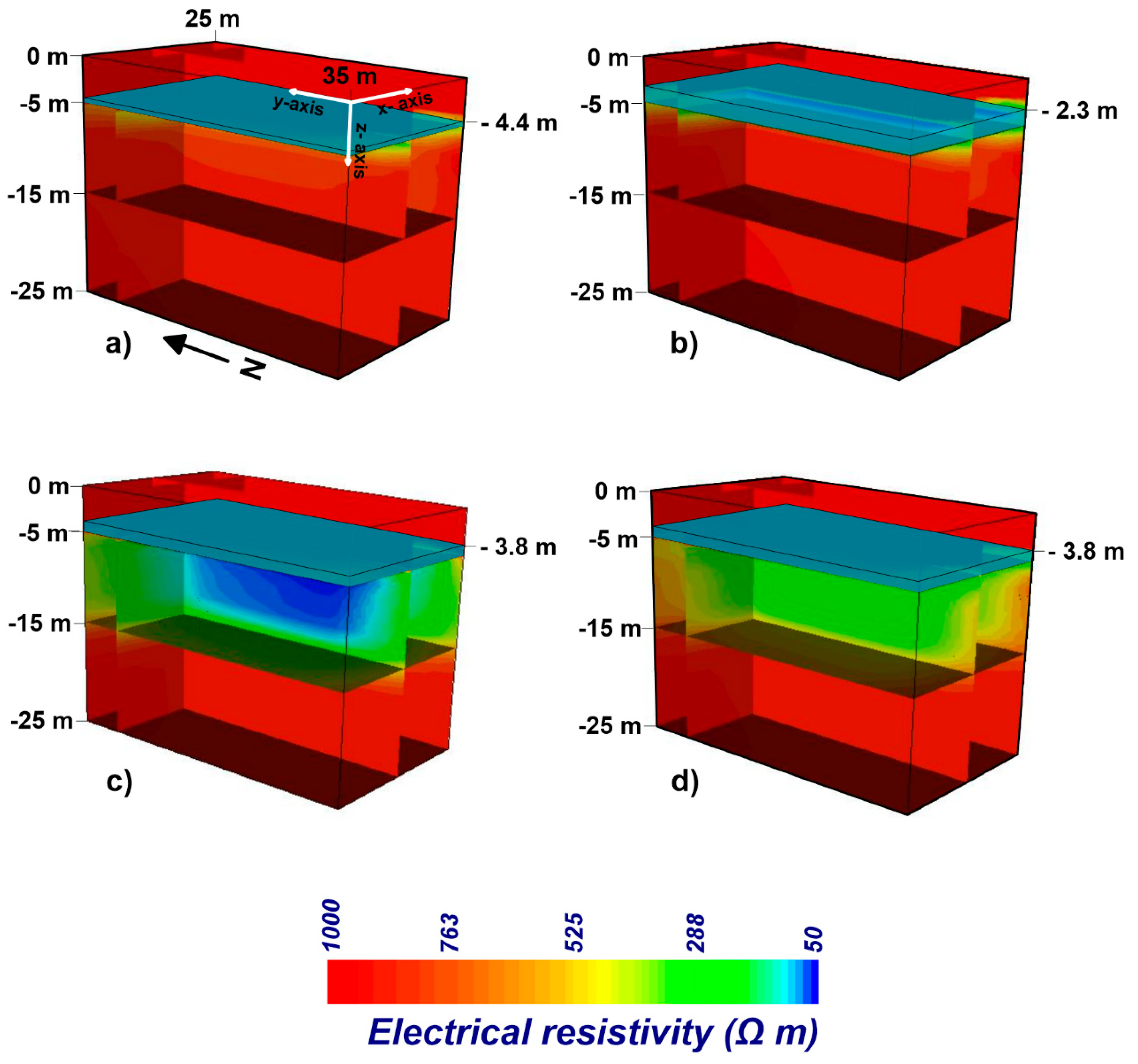
Figure 5 shows four inverted forward models obtained with different boundary conditions.
Figure 5a,b refers to the response models, assuming hydraulic heads are set to 0.60 m and 2.70 m;
Figure 5c,d is related to the response models when the hydraulic head was set to 1.20 m and resistivity perturbations of the upper subsurface, i.e., a 10-m-thick layer between −5 m and −15 m bgs, were set to 100 Ω m and 300 Ω m, respectively, corresponding to two different saturation degree conditions in the subsurface.
Despite the presence of the upper high resistivity air layer, for convenience the resistivity scale was set from 50 to 1000 Ω m in order to highlight the resistivity features below the bottom of the trench.
The response model shown in
Figure 5a,b is consistent with the assumed conceptual model, meaning that the current flow in the subsurface is minimally affected by the water height inside the trench. This could be due to the high interelectrode spacing (5 m) compared to the relatively small variations of the hydraulic head.
The inverted forward models shown in
Figure 5c,d capture well the assumed electrical signatures, meaning that the geophysical ERT tool can discriminate the significant changes in resistivity associated with water content variations in the given geometric layout.
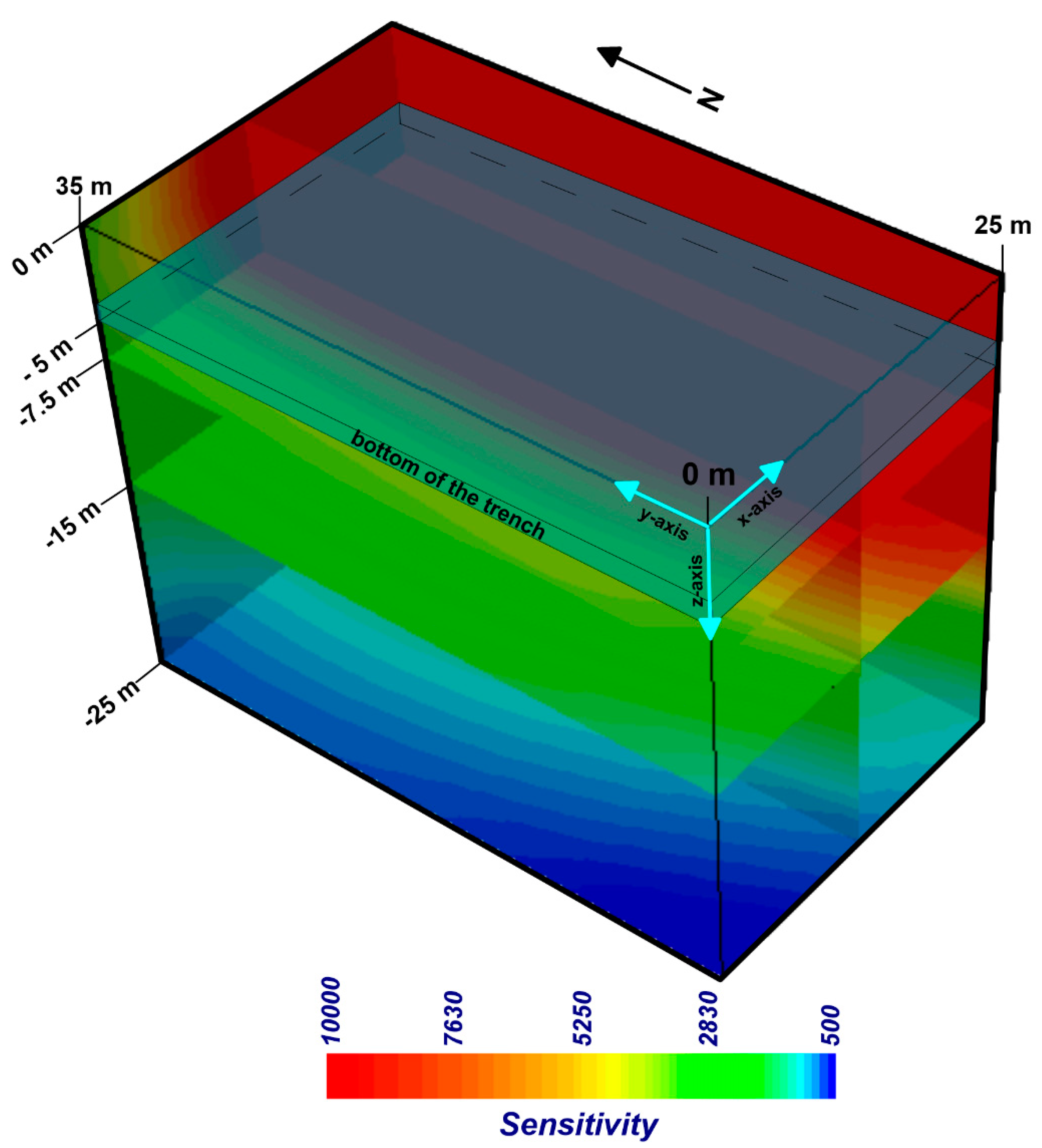
Figure 6 shows the 3D sensitivity map of a volume comprising the infiltration trench from the ground surface until about 25-m deep. Higher sensitivity values are recorded from the ground surface up to a depth of 15 m, meaning that, despite the unconventional configuration, this array can accurately detect vertical and horizontal changes below the trench bottom. A slight decrease toward the western part of the trench was recorded, while below 15 m the geophysical tool seems to be less effective at detecting resistivity variations, as expected.
In light of the considerations that emerged from the forward-modeling and sensitivity analysis, the time-lapse geophysical results were focused on drying–wetting dynamics within 15 m of the surface.
Furthermore, given the negligible effect of the hydraulic head inside the trench on subsurface resistivity distribution, a mean hydraulic head equal to 1.20 m was set as a boundary condition for each ERT snapshot dataset to perform the time-lapse resistivity ratios inversion.
4.3. ERT Monitoring Results
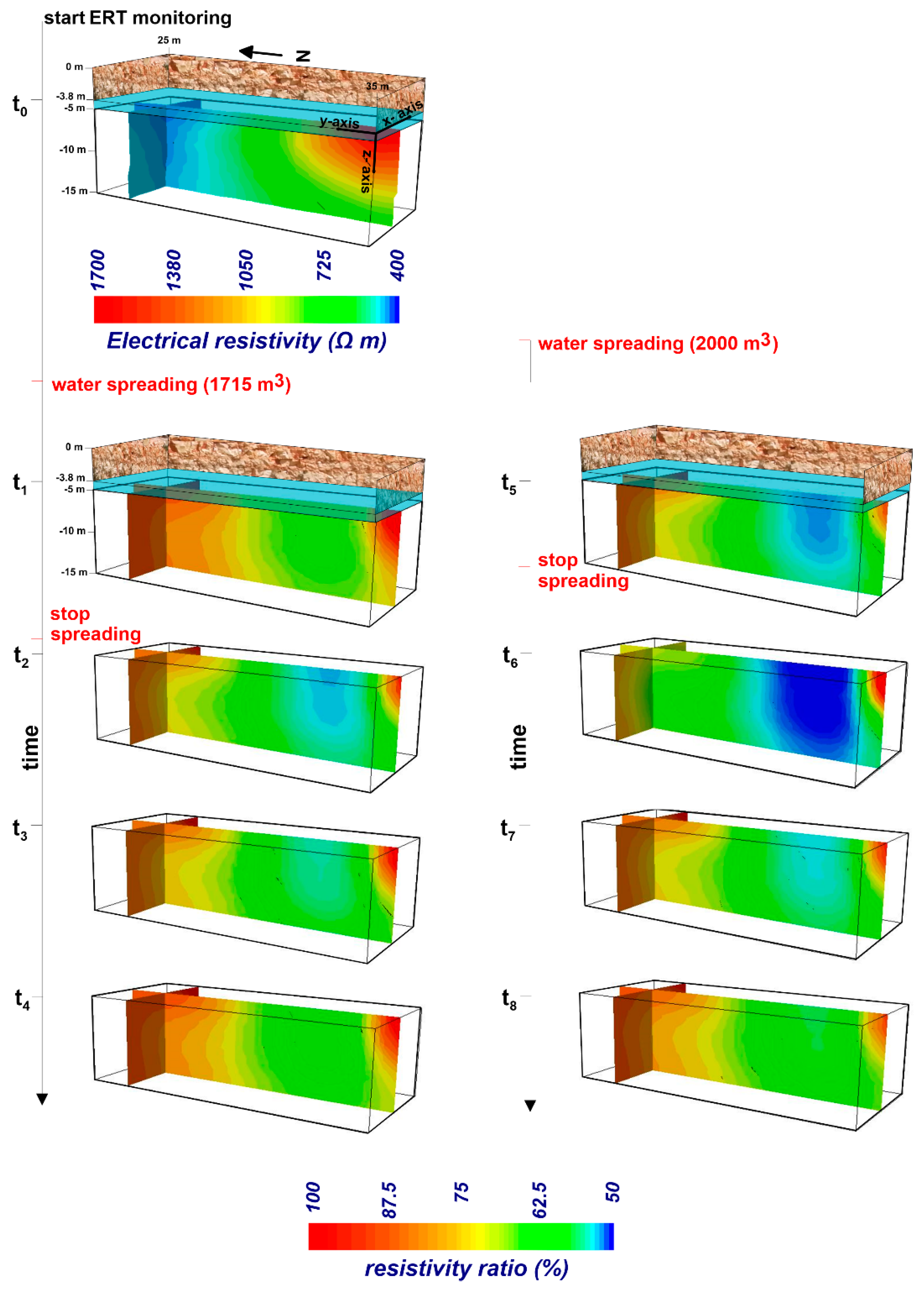
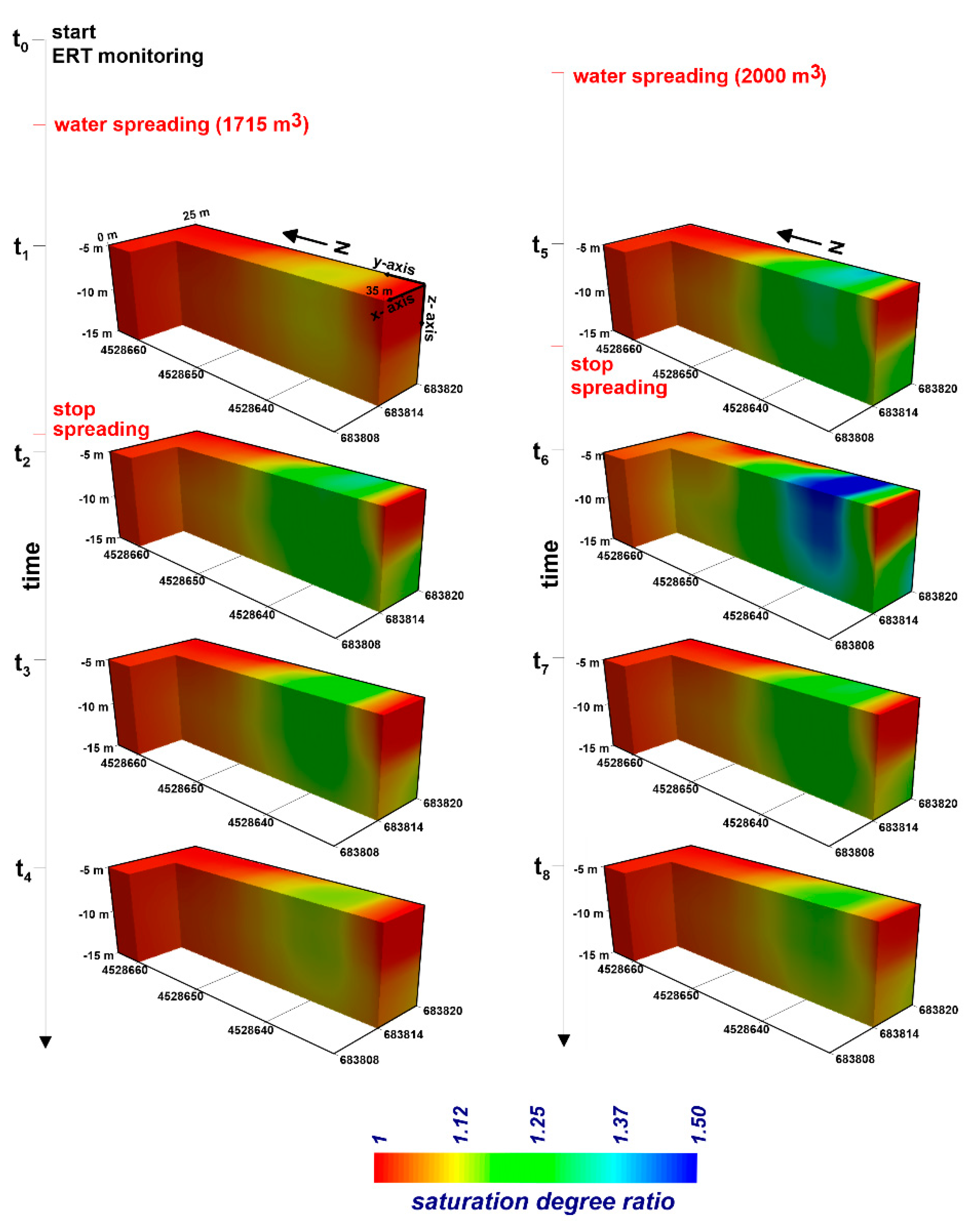
Figure 7 shows the resistivity changes recorded in March at eight time points, indicated with black arrows in
Figure 4. The background resistivity, corresponding to the reference resistivity with respect to which the comparison was made (
t0 on 22 March at 12:30), was also shown. At the start of the ERT monitoring the resistivity values ranged from 400 to 1700 Ω m, reflecting the water content conditions of the preceding wetting–drying cycle. In fact, the narrow temporal window considered for the geophysical monitoring is part of the cyclic wetting–drying dynamics that started in 2016. Given that the trench was always in operation and never emptied completely, a relative background resistivity was considered at the time point close to the minimum hydraulic head observed (h
0 = 0.39 m).
Times t1 and t5 correspond to the first dataset collected after each spread (19 h and 11 h, respectively) while the filling of the trench was still going on.
The resistivity scale is expressed as a percentage of resistivity variation with respect to the reference time: values equal to 100 correspond to unchanged resistivity, while values less or more than 100 represent a decreasing or increasing resistivity, respectively.
The resistivity ratio ranges from 50 to 100, meaning that the resistivity trend is always decreasing compared to the background resistivity; the resistivity changes reflect the water level trend inside the trench, when the water level increases, the resistivity ratio decreases, and vice versa.
The greater the amount of spread water in the second wetting cycle (2000 m3 compared with 1715 m3 in the first cycle), the greater the decrease in resistivity.
The resistivity variations are more enhanced in the south portion of the trench and reduced in the central and north part, where the discharge point is located.
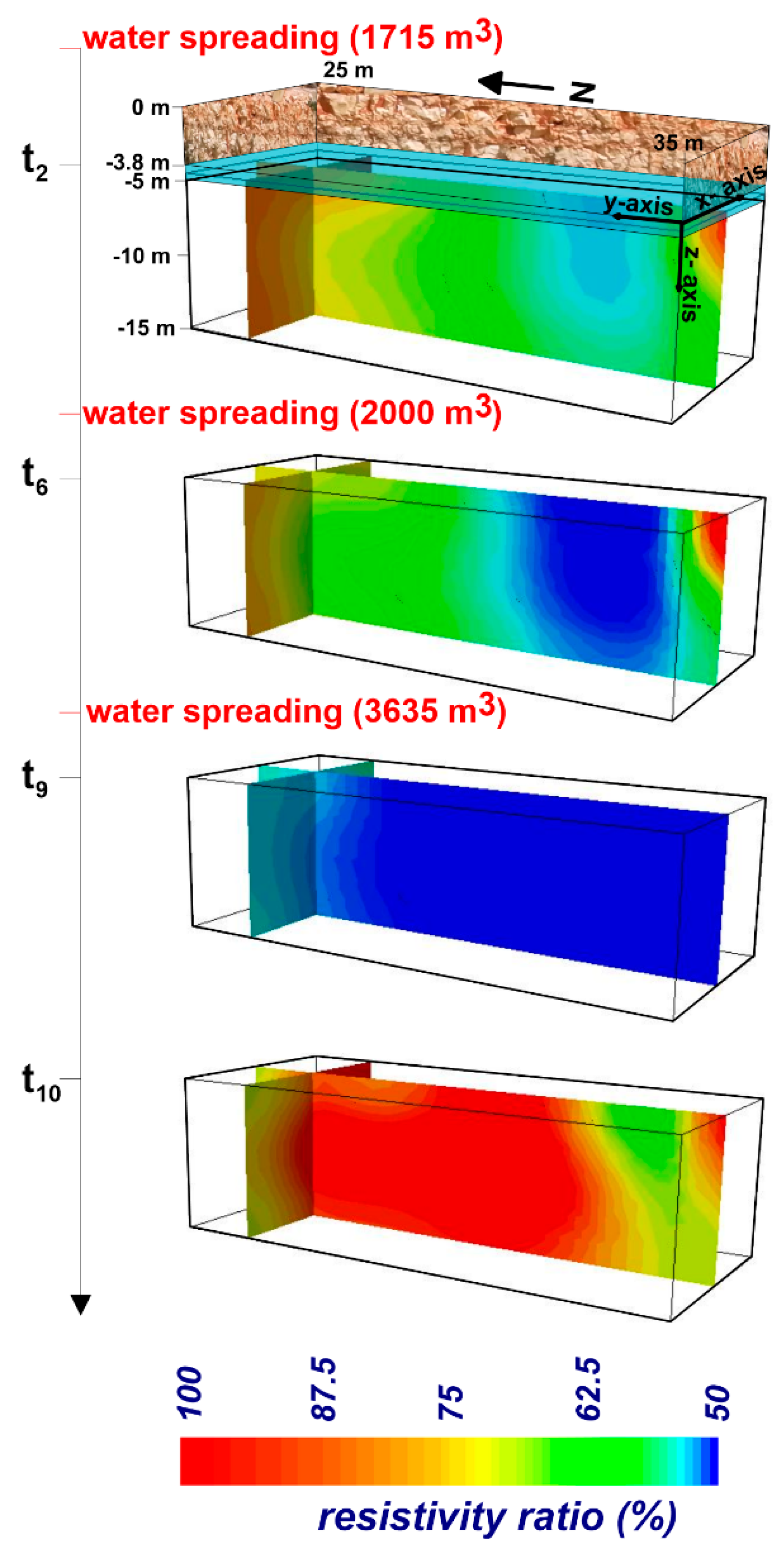
In July, due to logistical problems, it was not possible to monitor different wetting–drying phases as in March. In this case, the single spread of 3635 m3 of water, about the total amount of the two spreads monitored in March, happened about 32 h before the first ERT monitoring and, hence, only the effect of drying phase was captured.
In light of this consideration, the comparison between the results in March and July aimed to visualize the storage–release capability of the subsurface under quite different rock saturation conditions.
To enhance this feature, the resistivity ratio with respect to the reference time was imaged at four different time points (
Figure 8), two temporally placed in March (
t2 and
t6) and the other two in July (
t9 and
t10 indicated in
Figure 4).
In particular, the ERT changes were observed at the time points where the water level reached the maximum values in the trench (t2 and t9) or slightly less (t6). At the end of the ERT monitoring, the last image (t10) was used as a check point.
The resistivity patterns observed between the two test periods are clear. The resistivity decreased gradually at times
t2 and
t6, showing a heterogeneous pattern between the south and the north portions of the trench, as also shown in
Figure 7. Four months later, at time
t9, the resistivity ratio distribution reached its minimum value over the whole volume of interest, while later on, at time
t10, the resistivity tended to increase over the whole volume and returned to the background condition recorded in March.
4.4. Hydrological Implications
The resistivity ratios observed in
Figure 7 were converted into the ERT-derived saturation degree using the simplified Archie’s law (Equation (3)).
The subsurface saturation dynamics shown in
Figure 9 reflects a marked anisotropy of the fractured subsurface, during both the wetting and drying phases. At times
t1 and
t5, corresponding to the first dataset collected after the two spreads, a fast and enhanced response in terms of increased water storage was observed in the south part of the trench.
The higher the spread flow rate, the higher the increase in saturation. In fact, an increase of 50% in saturation was recorded at time t6, after the spread of 2000 m3, while a lower water spread caused a smaller increase in saturation, about 25%, recorded at time t2.
In both cases, when the spread stopped, the saturation degree decreased during the discharge phase.
The fast and enhanced response of the south part of the trench is ascribed to a more fractured and karstified area where the local anisotropy of the system, as verified by the high horizontal-to-vertical hydraulic conductivity ratio, plays a crucial role in the water dynamics, in both the inlet and discharge stages. In this portion of the trench, the fracture network alternatively fills up and empties very quickly, leading to fast saturation degree changes, expressed in terms of the ratio of saturation with respect to the background condition. In the drying phase, the saturation degree decreases due to the entrance of air into the fractures and consequently to the emptying of water from the fractures. The opposite situation is true of the wetting phase when the fracture system fills up with water.
On the other hand, in the north part of the trench, changes of less than 10% were observed during the whole monitoring period, probably due to the presence of the outlet and to the outcropping matrix-dominant rock that drains the spread water differently.
The heterogeneity of the rock system has great implications for the water flow dynamics.
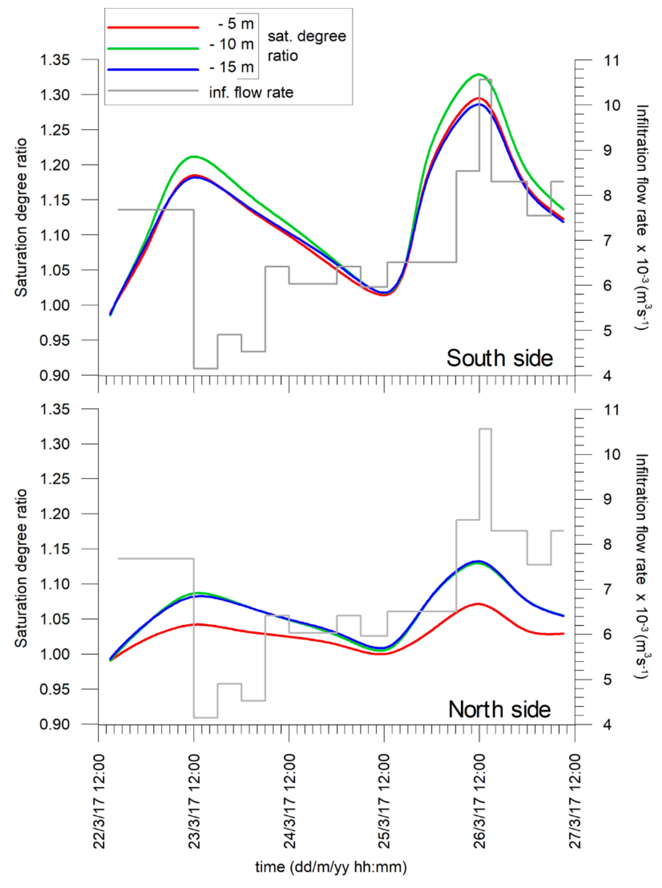
The different infiltration pattern between the south and north sides is clear in
Figure 10, where the saturation degree vs. infiltration flow rate was plotted. The saturation degree was calculated as the average of the values inferred from the ERT images in the north and south sides of the trench.
The graph provides further details about the space–time variability and flow anisotropy, not only in the horizontal, but also in the vertical direction.
Changes in saturation degree were observed in the trench at three different depths; on the south side, at a depth of −10 m bgs, an increase in drainage was recorded, probably due to a more fractured layer compared to the surrounding layers.
At the same time, on the north side, the saturation showed small variations, more marked at greater depths (−10 m and −15 m bgs).
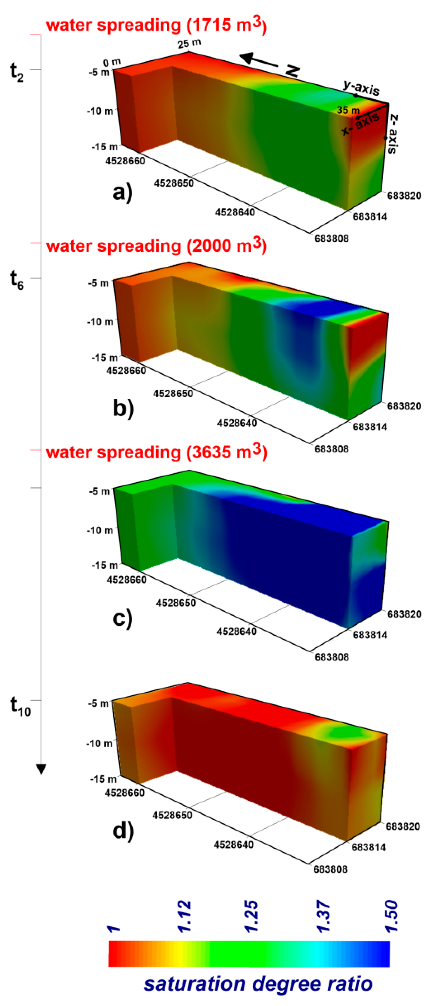
Furthermore, the correlation between the magnitude of the saturation changes and the amount of spread water is clearly visualized in
Figure 11, obtained by converting the ERT images shown in
Figure 8.
In July, the spread of 3653 m3 of water caused high subsurface saturation over the whole volume of the trench; in March, the second spread (2000 m3) caused higher saturation values than those recorded after the first spread (1715 m3), due to a higher starting value of subsurface saturation.
After four months of cyclic wetting–drying phases, at time t10, the saturation degree did not change significantly (except for a small portion located in the south part of the trench) compared with the background saturation conditions.
Figure 12 shows the infiltration efficiency vs. time observed in March for the two points located in the north and south portions of the trench. The water level is also shown in the graph.
According to Equation (4), the infiltration efficiency was calculated considering the maximum inverted electrical conductivity recorded at time t6, σ(t0) and the inverted electrical conductivities at time ti.
At the southern point, the infiltration efficiency decreased faster and more significantly than at the northern one, reaching losses of up to 80%, due to the presence of a more permeable layer in this part of the trench. On the contrary, the northern side preserves a high infiltration efficiency of more than 70%.
5. Discussion
The choice of the hydraulic operating conditions, including the amount of water to be spread and the time interval between subsequent different water spreads, is a crucial issue in the optimal management of infiltration trenches.
The spreading strategies affect the subsurface saturation degree and, consequently, the stored water volume and the infiltration flow rate, which control the residence times of water in the filtering medium as well as the infiltration efficiency of the trenches during the entire life cycle.
Moreover, the long-term settling of suspended material in the pore space can cause a clogging effect, leading to a reduction of the drainage capacity of the trench.
In the case of the use of infiltration trenches as final receptors for wastewater or as MAR plants, a broad-based experimental approach that takes into account the hydraulic response of these complex systems is strongly encouraged.
In our specific case study, the combined hydrogeophysical approach was able to evaluate losses in drainage capacity at different spatial and temporal scales.
In fact, in the two observation periods, a remarkable reduction in the trench-averaged infiltration flow rate, of about 35%, as estimated through the water level measurements, was observed. The infiltration estimates thus calculated are not suitable for investigating the subsurface heterogeneity, which could cause some areas of the trench to infiltrate much faster or slower than others or reveal whether parts of the trench are being preferentially affected by clogging. For this reason, the overall direct measurements were integrated with time-lapse geophysical data in order to gain more detailed information about the infiltration dynamics.
The geophysical monitoring highlighted significant variations in local infiltration efficiency due to the strong heterogeneity of the rocky subsurface within the trench.
Both the matrix-dominant portion and the highly fractured portion characterizing the filtering medium strongly affected the hydrological dynamics. More specifically, in the fracture system water flows quickly into the fracture network, leading to high infiltration rates. On the contrary, in matrix-dominant portion moisture dynamics occurs at a small pore scale and the water flow is strongly inhibited.
Although the hydrogeophysical monitoring was performed in a limited time window, this metric, combined with other traditional measurement systems, can provide real-time information at a local scale. At the same time, this approach, routinely used as a monitoring system, can be a promising tool to improve alert systems for the identification of clogging effects in the trenches.
6. Conclusions
This case study dealt with a hydrogeophysical approach for monitoring the drainage efficiency of infiltration trenches used as treated wastewater disposal.
The combined approach—between direct measurements such as infiltration flow rate measures and indirect investigations such as geophysical ones—proved to be a useful tool to study flow dynamics in the fractured and karstified vadose zone below the infiltration tranches, where high-resolution hydrological measurements are difficult to collect with traditional sensors.
On one hand, conventional water level measurements provide an average hydraulic response of the filtering medium below the trench, highlighting overall seasonal variations in the infiltration process in the short-term monitoring period. On the other hand, time-lapse ERT surveys showed the remarkable variability of infiltration dynamics during the wetting–drying dynamics.
Noninvasive geophysical investigations imaged different saturation conditions of the subsurface depending on the amount of spread water, with high spatial resolution.
Accurate predictions of the water storage capability are not a trivial issue because this parameter changes with the saturation degree, which, in turn, controls the infiltration rates into the system and, hence, the residence times of water in the vadose zone.
Moreover, geophysical datasets collected in the time-lapse mode can detect variations in the saturation degree over time and/or the anisotropy of water flow connected to the presence of strong heterogeneities in terms of geological structure such as differently karstified fractures. This is demonstrated by comparing the two areas of the monitored trench that show anisotropy in water flow due to different fracturing degrees.
This approach can adequately support the planning, implementation and operational phases of the infiltration trenches, in case of their application as MAR plants in fractured and karstified systems.
In the planning stage, detailed knowledge of the geological properties of the filtering medium can provide critical information about parameters controlling the infiltration rates.
At the same time, during the implementation and operational stages, an integrated approach can address best management practices in order to minimize the negative effects associated with clogging and hence optimize the life cycle of the infiltration trenches, including changes in the hydraulic operating conditions, such as adjusting volumes of water to be spread and varying the time interval between subsequent spreadings.


