Article

A Process-Based, Fully Distributed Soil Erosion and Sediment Transport Model for WRF-Hydro

1
Department of Oceanography and Coastal Sciences, Louisiana State University, Baton Rouge, LA 70803, USA
2
Center for Computation and Technology, Louisiana State University, Baton Rouge, LA 70803, USA
3
Coastal Studies Institute, Louisiana State University, Baton Rouge, LA 70803, USA
4
National Center for Atmospheric Research, Research Applications Laboratory, Boulder, CO 80305, USA
5
Weather Tech Services, LLC, Longmont, CO 80503, USA
6
School of Engineering, National Autonomous University of Mexico, Mexico City CP 04510, Mexico
*
Author to whom correspondence should be addressed.
Water 2020, 12(6), 1840; https://doi.org/10.3390/w12061840
Submission received: 18 April 2020 / Revised: 22 June 2020 / Accepted: 24 June 2020 / Published: 26 June 2020
(This article belongs to the Special Issue Modeling of Soil Erosion and Sediment Transport)

Abstract

:
A soil erosion and sediment transport model (WRF-Hydro-Sed) is introduced to WRF-Hydro. As a process-based, fully distributed soil erosion model, WRF-Hydro-Sed accounts for both overland and channel processes. Model performance is evaluated using observed rain gauge, streamflow, and sediment concentration data during rainfall events in the Goodwin Creek Experimental Watershed in Mississippi, USA. Both streamflow and sediment yield can be calibrated and validated successfully at a watershed scale during rainfall events. Further discussion reveals the model’s uncertainty and the applicability of calibrated hydro- and sediment parameters to different events. While an intensive calibration over multiple events can improve the model’s performance to a certain degree compared with single event-based calibration, it might not be an optimal strategy to carry out considering the tremendous computational resources needed.

1. Introduction

Eroded by different forcing agents, soil is being lost at a rate that is orders-of-magnitude greater than its replenishment [1]. Among all the erosive agents, water is the most prevalent and usually dominates. Moreover, due to the current climate change, the frequency, and the intensity of extreme rainfall events are projected to increase, which will lead to more intensive erosion [2]. With this in mind, a lot of soil erosion models have been developed to mainly simulate water-induced erosion. Based on the numerical algorithms applied, these models can be classified as conceptual, empirical, and process-based models [3]. The latter, with detailed representation of physical processes, is becoming the mainstream in both academia and industry [4].
Depending on how processes and parameters are described, process-based models can be further grouped into semi-distributed and fully distributed models. Semi-distributed models, such as CREAMS (Chemical Runoff and Erosion from Agricultural Management Systems model [5]), WEPP (Watershed Erosion Prediction Project [6]), EUROSEM (EUROpean Soil Erosion Model [7]), KINEROS (KINematic EROsion Simulation [8]), and THREW (TsingHua Representative Elementary Watershed [9]) break down the model domain (a watershed or a catchment) into a series of basic elements such as hillslopes, planes and channels, over which the algorithms are applied and physical parameters are represented [10]. However, since hydrological parameters are lumped over the basic elements, semi-distributed models are not able to fully account for spatial heterogeneity. Fully distributed models divide a study domain into grid cells with certain sizes. The spatially distributed input data of fully distributed models are usually generated by the Geographical Information System (GIS). In this way, the physical heterogeneity is better represented. With the advances of scientific computation, several fully distributed, process-based models have been developed over the past three decades. Notable examples are LISEM (LImburg Soil Erosion Model [11]), SHESED [12] and CASC2D-SED (CASCade 2 dimensional sediment model [13]). Recently, a physically based hydrological and soil erosion model has been developed by coupling the Soil Conservation Service model with a 2D fully Dynamic Wave model and a Hillslope Erosion model by Juez et al. [2] The model is applied over a Mediterranean watershed to simulate the rainfall-runoff and soil erosion process during two rainfall events with satisfactory results generated. An efficient approach has been applied on the model for calibration process, which has largely reduced the computational cost. The model has demonstrated its potential applicability to large and long-term scale hydro-sedimentary process studies under climate change [2]. In addition, the distributed model usually simulates the sedimentary processes in 2D mode. In the study of the replenishment of sediments in a water-worked channel using the 2D shallow water equation model coupled with Exner equation, Juez points out that the 2D distributed model can better resolve the bidimensional water and sediment flux compared to the 1D model [14]. Moreover, the 2D model is more computationally efficient than the complicated 3D model while still meeting research and engineering requirements [14].
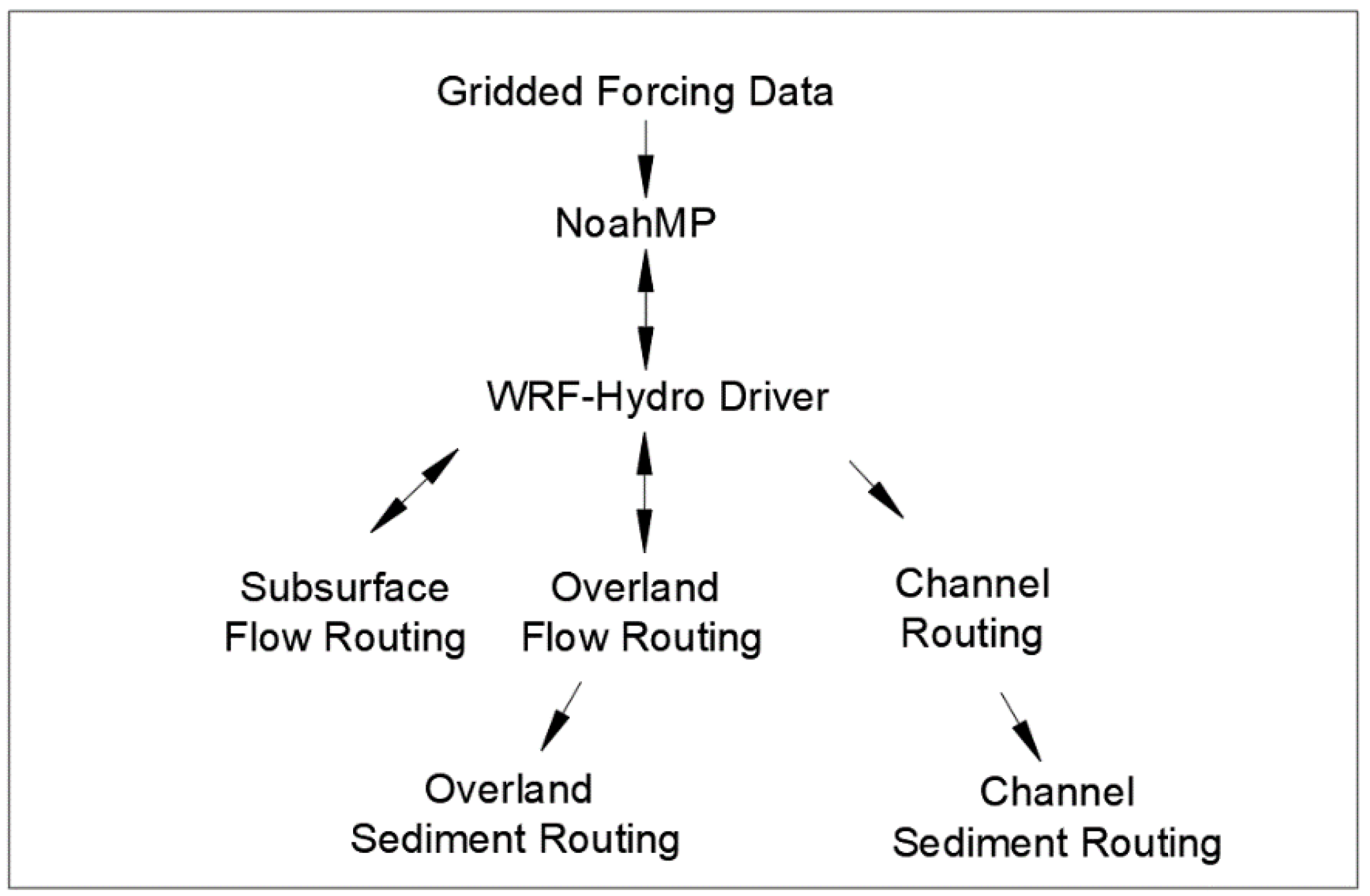
In this study, we present a newly developed, fully distributed, process-based soil erosion and sediment transport model. Our model is built on WRF-Hydro, which simulates the hydrological cycle and provides hydraulic parameters for soil erosion and transport. WRF-Hydro was developed as the hydrological modeling extension package of WRF at the National Center for Atmospheric Research in Boulder, Colorado [15]. Compared to other hydrological models such as the Variable Infiltration Capacity model (VIC, [16]) and the Soil and Water Assessment Tool (SWAT, [17]) model, WRF-Hydro’s advantage is its capability of simulating multi-processes at multi-scales while considering the spatial distribution of hydrological variables. Besides, WRF-Hydro takes advantage of various available meteorological and terrain datasets and has been fully coupled with meteorological and climate models such as WRF. WRF-Hydro’s performance has been evaluated by its applications in flooding [18], water resource management [19], water budget estimation [20], decadal scale hydroclimatic change [21], and others. Currently, an instance of WRF-Hydro is running operationally as the National Oceanic and Atmospheric Administration’s (NOAA) National Water Model, which provides streamflow forecasts on 2.7 million river reaches of the contiguous United States. However, until this study, WRF-Hydro does not include a sediment module, which limits its capability in water quality-related forecasts and studies.
In this paper, the architecture and algorithms of the WRF-Hydro-Sed model, the study area, and datasets used as well as the calibration method are presented in Section 2. Results of model calibration and validation are detailed in Section 3. Section 4 discusses the model’s uncertainty, the validity of applying calibrated parameters to different events, the relationship between landscape patterns and soil erosion as well as the limitation of current model regarding long-term simulation under climate change. A conclusion is given in Section 5.

2. Materials and Methods

2.1. WRF-Hydro

The structure and schematic representation of WRF-Hydro-Sed are shown in Figure 1; Figure 2, respectively. WRF-Hydro is an integrated modeling platform that incorporates a land surface model (LSM), grid aggregation/disaggregation, subsurface flow routing, surface overland flow routing, channel routing, lake and reservoir routing, and a conceptual base flow model. In this study the soil erosion and sediment transport processes are built on WRF-Hydro’s overland flow and channel flow routings.

2.1.1. Overland Flow Routing

In WRF-Hydro, the surface runoff is generated through infiltration-excess and saturation-excess of a supersaturated soil column. It can be routed either two-way or one-way (along the largest gradient of slope), depending on the routing method specified in the model name list. As the physics and algorithms of both routing options are identical, only the equations used for two-way routing are presented here. The overland flow is assumed to be fully unsteady and non-uniform. The diffusive wave formulation, which is a simplification of Saint-Venant equations for a shallow water wave, is applied:
Continuity Equation:
h t + q x x + q y y = i e
Momentum Equation:
S f x = S o x h x S f y = S o y h y
where h is the surface flow depth (L), q x , q y are the unit discharge in x and y direction, respectively (L2 T−1) (in 1-way routing only discharge in the steepest direction is calculated), and i e is the infiltration excess (L T−1). S f x , S f y are the friction slope in x and y directions, S o x ,   S o y are the bed slope in x and y directions, and h x , h y are the gradient of surface flow depth in x and y directions.
Manning’s equation is used to calculate q x and q y in order to solve Equation (1),
q = α h β ,   β = 5 / 3 α = S f 1 / 2 n
where q is the unit discharge in x or y direction (L2 T−1), h is the surface flow depth (L), S f is the friction slope in x or y direction, n is the Manning roughness coefficient of land surface.
Since WRF-Hydro’s performance is steady with the one-way routing in a parallel mode, we use the one-way overland routing method to simulate overland flow and provide the hydraulic parameters needed to drive the sediment model.

2.1.2. Channel Flow Routing

Once overland flow gets into the channel network, the water will be routed as channel flow. Currently, WRF-Hydro provides three channel routing options: Muskingum, Muskingum-Cunge, and Diffusive Wave Routing. As the first two options are usually applied for vector-based reaches, we use the third option for gridded channel routing. An explicit, one-dimensional, variable time-stepping diffusive wave formulation is used as follows:
Continuity Equation:
A t + Q x = q l a t
Momentum Equation:
Z x = S f
where A is the cross-section area (L2), t is the time (T), Q is the flow discharge, which is the product of cross-section area and mean flow velocity perpendicular to cross-section area (L3 T−1),   q l a t is the unit discharge of the lateral flow (L2 T−1), Z is the water surface elevation, which is the sum of bed elevation and water depth (L),   S f is the friction slope.
The friction slope S f is solved as follows:
S f = ( Q K ) 2
K = C m   n   A R 2 3
where K is the flow conveyance coefficient (L3 T−1), C m is the dimensional constant (1.0 for SI units), n is the Manning roughness coefficient, R is the hydraulic radius (L).

2.2. Soil Erosion and Sediment Transport Model

The sediment algorithm is adapted from the CASC2D-SED model, which is a fully distributed, physically based hydrological and upland erosion model developed at Colorado State University. CASC2D-SED is capable of reproducing hydrograph and sediment graph at different grid scales [22]. The code is converted from C to Fortran, and then incorporated into WRF-Hydro as an independent module.
On watershed scale, the annual gross erosion includes upland erosion, gully erosion as well as local bank erosion [13]. In the model, three sediment size groups—sand, silt, and clay—are included. Each sediment group can be presented in three states: suspended, deposited, or in bed layer. The bed layer represents the original soil layer and thus serves as the source of the sediment to the model domain. Once eroded from the bed layer, the sediment becomes suspended. After settling down, it goes into deposited.
As shown in Figure 2, sediment is first eroded from and transported through overland area by surface runoff. At the beginning of each time step, the total transport capacity is calculated with the revised USLE [23] over upland area. With the transport capacity, the suspended sediment is transported first, followed by the deposited part. At last, if there is still transport capacity left (excessive transport capacity), it will be used to erode the bed layer. During these processes, both the wash load and bed load transportation are considered. The different treatment of transport of the fine materials as wash load and coarse materials as bed load are achieved mainly by assigning different settling velocities to different sediment size groups.
In the channel, the sediment is carried by streamflow through the river network delineated in the model, meanwhile settling and resuspension processes are calculated. According to the Engelund and Hansen (1967) equation [24], the transport capacity is calculated for each sediment group separately in the channel. With the transport capacity, the suspended part of each sediment group is transported first by advective process. Then, bed material will be transported with excessive capacity. Channel erosion is not considered by the model yet. The different treatment of fine materials and coarse materials is accomplished by the differences in transport capacity as well as settling velocity between sediment groups.
Once sediment is transported from the “source grid (where the sediment comes from)” to the “sink grid (where the sediment goes to)”, all the transported materials will stay in suspension first and then settle down at assigned settling velocities. By the end of each computational step, the deposited sediment is added to the original layer and the net accretion/erosion is updated.

2.2.1. Overland Sediment Routing

The revised USLE [23] is applied to predict soil loss from upland area (sheet and rill), which is caused by rainfall and associated overland flow. In a single grid, the transport capacity is calculated as follows:
T o v r l = 58390 × S o 1.664 × q 2.035 × K × C × P × d x × d t
where T o v r l is the overland transport capacity (L3), here in the model m3,   q is the unit flow discharge (L2 T−1), in this study m2/s, K is the soil erodibility factor, which is in t/acre, C is the dimensionless cropping-management factor, P is the conservation practice factor, which is dimensionless, d x is the grid size (L), which is m in this study, and d t is the time step (T), which is in second. In this study, d x and d t are the same as those used in overland routing. S o is the water surface slope. The overland sediment transport capacity is used to transport suspended sediment first, and then the deposited sediment if any. After the suspended and deposited sediment in the source grid are transported, if there is still transport capacity left, the remaining capacity will be used to erode the original bed layer.

2.2.2. Channel Sediment Routing

The Engelund and Hansen (1967) [24] equation is applied to calculate the sediment transport capacity for each sediment size group in channels. For each size group, the suspended part is transported by advective process first and the transport capacity will be subtracted by the amount of the suspended sediment transported. Then, the excessive capacity is used to transport deposited material. The amount of the deposited material that can be transported is limited by excessive transport capacity as well as advective processes. After the transport of suspended material and deposited material, if there is still any transport capacity left, it won’t be used as channel erosion is not considered in the current version of the model.
T i = Q × C i × d t 2.65
C i = 0.05 × ( G G 1 ) × V × S f ( G 1 ) × g × d i × R h × S f ( G 1 ) × d i
where T i is the sediment transport capacity in the channel for sediment type i (L3), Q is the flow discharge (L3 T−1),   C i is the sediment concentration of type i   by   weight ,   d t is the time step of channel routing (T), G is the specific gravity of sediment and was set to 2.65 in this study, V is the depth-averaged velocity in channel (L T−1), S f is the friction slope, R h is the hydraulic radius (L), g is the gravity acceleration (L T−2), d i is the diameter of sediment type i (L). Calculated transport capacity is used to transport the suspended sediment first and then the previously deposited sediment.

2.3. Study Site and Data Availability

We applied the WRF-Hydro-Sed model on the Goodwin Creek Experimental Watershed (GCEW), Mississippi, USA to assess its performance (Figure 3). GCEW is located at northwest Mississippi, close to Batesville. The watershed has a drainage area of 21.3 km2 with an outlet located at its southwest corner (89°54′50″ W, 34°13′55″ N). The Goodwin Creek is a tributary of the Long Creek, which flows into the Yocona River, one of the main rivers of the Yazoo River Basin [13]. The weather is hot and humid in summer and mild in winter, with an average annual rainfall of 1440 mm and a mean annual runoff of 145 mm during 1982 to 1992 [9]. Within the watershed, the elevation ranges from 68 m to 130 m above sea level. Around 50 percent of the watershed has a slope less than 0.02 and 15 percent has a slope larger than 0.03 [9]. The channels in the watershed extend mainly from northeast to southwest with an average slope of 0.004. Based on the State Soil Geographic Database [25], soils within the watershed are mainly silt loam and sandy loam, with the former one dominating. According to the 24-category Land Use Categories by the U.S. Geological Survey (USGS), the most common land cover types in this watershed are “dryland cropland and pasture”, “irrigated cropland and pasture”, and “deciduous broadleaf forest”.
GCEW was originally established in 1977 and has been operated by the U.S. Department of Agriculture (USDA) National Sedimentation Laboratory (NSL) to study the influence of land use and upland erosion on sedimentary process and channel stability and to test numerical models. It is highly instrumented, with 32 standard recording rain gauges distributed uniformly within the watershed, 14 stream gages and supercritical flow structures located along the channel to collect discharge and sediment concentration data. In addition, periodic surveys are conducted to track land use conditions, channel geometry, and channel migration. In this study, rainfall data from 16 rain gauges and the streamflow and sediment concentration data at the outlet (MSGC1) was collected to calibrate and validate the model (Figure 3). The data interval is ~15 min.

2.4. Model Setup

WRF-Hydro supports the coupling between hydrological components and atmospheric models. However, as the focus of this study is to introduce the sediment module instead of investigating the interaction between atmosphere and hydrological processes, WRF-Hydro is used in a “one-way coupled” mode.
The Noah land surface model with multi-parameterization options (Noah-MP) [27] is responsible for simulating land surface physics in the model (Figure 1). In this study, Noah-MP has a domain of 14 km × 11 km with a spatial resolution of 1 km. To drive the land surface model, static land surface physiographic data was generated using the WRF Pre-processing System (WPS). The land use information was interpolated from the 24-category USGS land use database derived from the 1-km Advanced Very High Resolution Radiometer (AVHRR) satellite images [28].
The meteorological forcing data is from the North American Land Data Assimilation System Phase 2 Forcing Dataset (NLDAS-2 hereafter, [29]). NLDAS-2 contains incoming longwave and shortwave radiation, near surface wind, specific humidity, air temperature, surface pressure as well as rainfall intensity with hourly temporal resolution. In this study, the 1/8-degree NLDAS-2 was regridded to 1 km to match the Noah-MP grid. Given its coarse resolution, the rainfall intensity of NLDAS-2 might not be able to fully represent the condition of such a small watershed. Therefore, we replaced NLDAS-2′s original rainfall data field with interpolated precipitation from the records at the 16 rain gauges using the inverse distance weighting interpolation method.
With a disaggregation factor of 20, the hydrological physical processes are simulated at the spatial resolution of 50 m. The subsurface routing, overland routing and channel routing of WRF-Hydro are all activated. The time step of the overland routing and channel routing is six seconds. Since the sediment processes are driven by the overland flow and channel flow, the setup of the sediment model highly depends on that of the hydrological model. The sediment model is calculated on the same grid as the hydrological model (50 m), with a time step of six seconds as well. Model tests and simulation were carried out on Louisiana Optical Network Initiative (LONI)’s QB2 and NCAR’s Cheyenne super computers. In a serial mode, it took 2.5 h to conduct a 2-year simulation of streamflow with sediment module deactivated, and 30 min to finish a 24 h sediment simulation.

2.5. Model Calibration

In this study, the streamflow, sediment concentration, sediment flux and sediment yield were selected as the major variables to calibrate and validate the hydro- and sediment model. A stepwise calibration was performed where first the hydro-parameters and then the sedimentation parameters were calibrated. The streamflow was calibrated first manually through trial and error, and then automatically using the NCAR developed calibration toolbox, which is based on the Dynamically Dimensioned Search (DDS) calibration methodology [30]. Once finished, the calibrated hydro-parameters were used to drive the sediment module and the sediment parameters were then calibrated manually.

2.5.1. Streamflow Calibration

Streamflow was calibrated for a 3-year rainfall event on 17 October 1981 (calibration event hereafter), which started at 21:19 and lasted for approximately five hours. The average rainfall intensity is 14.7 mm/h and total rainfall is 74.4 mm. Calibrated hydro-parameters were selected based on sensitivity analysis and previous studies [23,31,32].
The calibration was carried out through two ways: automated calibration using the NCAR developed calibration toolbox and manual calibration based on trial and error. The reason for calibrating the model in two ways is that the automated calibration tools, which are usually based on standard objective metrics, may weigh more on timing error while weighing less on amplitude error, or the other way around, and thus may result in unreasonable results [33]. A manual evaluation, if executed in a rational way, can take the advantage of both visual inspection and standard metrics. While laborious and highly dependent on researchers’ experience, the manual calibration may produce a better result.
Before calibration, a two-year run was performed starting from 1 January 1981 to let the model reach an equilibrium state before the calibration rainfall event. The results from each calibration were statistically evaluated using the correlation coefficient, Root Mean Square Error (RMSE), Nash-Sutcliffe coefficient (NSE) and Kling-Gupta efficiency (KGE). A detailed description of relevant equations is provided in the Supplementary Materials.
The Dynamically Dimensioned Search tool [30] was used for automated calibration. The objective function is the weighted NSE and logNSE:
O b j F n = 0 ( N S E 2 + log N S E 2 )
N S E = 1 t = 1 T ( O t P t ) 2 t = 1 T ( O t O t ¯ ) 2   
where N S E is the Nash-Sutcliffe coefficient, O t is the observed streamflow at time t, P t is the modeled streamflow at time t, O t ¯ is the average of observed streamflow.
Table 1 summarizes the hydro-parameters calibrated by automated calibration with their lower and upper limits and default values. These parameters are mostly related to the land surface model. The hydro-parameters were adjusted within a reasonable bound of values through a 300-iteration automated run. With 32 processors, it took 10 h to finish the automated calibration.
For manual calibration, the refkdt and RETDEPRTFAC in Table 1 were selected as they were identified as the most sensitive parameters by the automated calibration and previous studies [23,31,32]. In addition, channel parameters including channel bottom width (Bw) in meters, channel side slope (Chsslp) and Manning roughness coefficient (MannN) were also calibrated.

2.5.2. Sediment Calibration

Sediment concentration, sediment flux, and sediment yield were calibrated manually via a series of sensitivity tests following previous studies [9,13,23,34]. Calibrated sediment parameters can be categorized into two groups: soil-type related and land-use-type related. Soil erodibility factor K is soil-type related, while cropping-management factor C and conservation practice factor P are considered to be land-use determined. The calibrated sediment parameters are shown in Table 2.

3. Results

3.1. Streamflow Calibration

The best results from the automated and manual calibration at the outlet of GCEW are shown in Figure 4 and the related values of statistical metrics are in Table 3. Overall, both automatically and manually calibrated hydrographs exhibit a satisfactory performance with a high correlation coefficient (>0.90), NSE (>0.70) and a low RMSE (<8 m3/s). However, total amount of runoff is overestimated by both manual and automated calibration. While the automatically calibrated total volume of runoff is closer to observation, manually calibrated hydrograph fits better with the observed one over the high flow part of the measured hydrograph around the peaking time. As GCEW is self-drained watershed, we assume that large river discharge corresponds to large overland runoff flux. With the exponential relationship between overland runoff flux and transport capacity (Equation (8)), the sediment concentration and sediment flux during high flow periods should be much larger than during low flow periods. In this case, during a single rainfall event, the sediment concentration, flux, and total yield ought to be dominated by high flow period of the runoff event. (The observed sediment concentration and sediment flux graphs shown in Figure 5a,b justified this assumption as the main sediment event only lasted two hours, which corresponds to the high flow duration in the observed hydrograph shown in Figure 4). In this case, although the total volume from the automated calibration is closer to observation than the manually calibrated one, we chose to use the manually calibrated hydro-parameters to drive the sediment model since the high flow part of the manually calibrated hydrograph is much closer to observation. The values of manually calibrated hydro-parameters are shown in Table 4.

3.2. Sediment Calibration

Sediment concentration and sediment flux results are shown in Table 5 and Figure 5. Overall, the sediment concentration and sediment flux show good agreement with measurements at the outlet, indicating that the model can well reproduce the sediment erosion and transport processes on a watershed scale. Compared with streamflow, sediment concentration and sediment flux are less well predicted, with the NSE value of 0.25 and 0.28, respectively. For both sediment concentration and sediment flux, the simulated rising limbs fit well with the measured ones, while the peak values are underestimated. The falling limbs recess earlier but last longer. The long recession should inherit from that of the streamflow, and essentially the overland flow. The total sediment yield simulated during this event is around 9600 tons, which is 40 percent lower than the measurement. This error is close to the one reported by [13], which is considered to be acceptable in hydrological engineering.
We notice that the model simulated only one peak for sediment flux and sediment concentration, while the observation exhibited multiple peaks (Figure 5). Such a mismatch can be attributed to the uncertainty of observation or limitation of model algorithm. Due to the large fluctuation of sediment concentration during a rainfall event, the point-wise observation data might not be able to detect the real condition of sediment concentration. Thus, the multiple peaks shown in Figure 5 might not be the real case. If we assume that the observed multiple peaks are the real condition, the multiple peaks or rapid fluctuation of the sediment concentration and sediment flux might be attributed to local erosion of channel or bank collapse, which are currently not represented in the model.

3.3. Model Validation

Using calibrated parameters, we validated the model performance on the rainfall event of 28 August 1982. The return period of the event is one year. It started at 23:30 and lasted 4.5 h with an average rainfall intensity of 10.4 mm/h. The simulation was initialized on 1 January 1981 to assure the model reached a relatively stable condition before the rainfall event. Figure 6 shows the simulated and measured hydrographs at the outlet. The model was able to reproduce the measured hydrograph. The statistical results shown in Table 6 indicate satisfactory simulation skill of the model with a high NSE (0.86). We notice that the simulated rising limb starts earlier than the measurement and the falling limb drops slowly and lasts longer. The simulated peak is within 20 min of the measured one and the simulated peak value (27 m3/s) is 26 percent lower than the measurement (36.4 m3/s). Simulated water discharge at the outlet is within 10 percent of the measurement.
The comparison between simulated and measured sediment concentration and sediment flux is shown in Figure 7. The model can catch the shape of the observed sediment graphs but with an overall overestimation for both sediment concentration and flux. Sediment flux is better simulated than sediment concentration with NSE and KGE 0.09 (vs. −2.26 for concentration) and 0.34 (vs. −0.15 for concentration), respectively. A comparable model performance in sediment concentration simulation is also reported by Elliot [35], which was partially attributed to the fact that simulation of sediment concentration involves an error in both sediment simulation and runoff simulation. Due to the absence of observation data before 2:00, 28 August 1982, it is impossible to calculate the sediment yield during the entire event. Yet it is reasonable to assume that the real sediment yield is larger than the estimation based on the available data (9100 t). Thus, we consider that our model-simulated sediment yield (14,950 t) is acceptable.
In spite of the acceptable performance of the model in simulating the sediment yield for both events, the model tends to overestimate the sediment yield for validation events while underestimating it for calibration events. This difference in model behavior should be partly due to the difference in initial soil conditions of the two events. According to Rojas [23], the initial soil condition could be much wetter during the validation event, since a series of preceding rainfall events brought >110 mm rain in the previous month. Yet there was only one preceding rainfall event bringing ~15 mm rainfall before the calibration event. In this case, the soil erodibility factor calibrated for the calibration event might be too large for the validation event, as soil erodibility tends to be smaller in wet conditions than in dry conditions [36]. Thus, the sediment yield during the validation event is overestimated by the model.

4. Discussion

4.1. Unceratinty Quantification

For the hydrologic simulation, uncertainty can result from different sources such as forcing data, model structure, model parameter, and initial and boundary condition uncertainties [37]. Each of these sources of uncertainty could be investigated and reduced through different treatments such as by providing more accurate forcing data to reduce the forcing uncertainty or by calibrating the model parameters to limit the parameter uncertainty. Data assimilation techniques are also used commonly to reduce the uncertainty due to the initial and boundary conditions in the models and in some cases to address the parameter uncertainty. Although investigating the model structure uncertainty is possible via the multi-parameterization scheme of NoahMP as the Land Surface Model used in WRF-Hydro as well as through different routing options available in WRF-Hydro, such a study was beyond the scope of this paper. We investigated the impact of the forcing on the model simulation as well as the parameter uncertainty, a subset of sources of uncertainty, of which the findings are summarized in the following subsections.

4.1.1. Forcing Uncertainty

Poor representation of meteorological forcing or errors may propagate into the hydrologic simulation and affect the result in a nonlinear way. Similar to previous WRF-Hydro studies [20,21], the NLDAS-2 dataset was used in this study as meteorological forcing. As explained in Section 2.4, in order to better represent the rainfall intensity, NLDAS-2′s rainfall field was substituted with interpolated rain gauge observation. However, how well the model can perform when driven by the original NLDAS-2 dataset needs to be investigated. We performed a sensitivity experiment on the calibration event. The streamflow was simulated with default parameters (un-calibrated) and driven by the original NLDAS-2 (1/8 degree resolution) and updated rain gauge data (1 km resolution), respectively. The comparison between simulated and observed hydrographs is shown in Figure 8.
Without calibration, using the original NLDAS-2 forcing data, the simulated hydrograph (Figure 8, dash-dotted line) fails to reproduce the rainfall event. Once the rainfall field is updated with rain gauge data and used to drive the model, a significant improvement is achieved in terms of amplitude of simulated hydrograph (Figure 8, solid line). However, timing error still exists, which will be largely minimized through calibration, as shown in Figure 4. A similar improvement has also been reported previously [37]. Thus, rainfall data with compatible resolution is recommended when applying WRF-Hydro-Sed to a relatively small watershed under local storm events in order to generate satisfactory results. This comparison could serve as a good example of how sensitive the model response is to the forcing dataset and in this case, precipitation. Ideally, one would like to force the model with an ensemble of the different forcing datasets to cover a range of forcing uncertainty in the model simulations.

4.1.2. Parameter Uncertainty

Model parameters are another source of uncertainty in the model simulation. This uncertainty is reduced to some degree through the calibration process. In this part, based on the single event calibration, we assess the goodness of calibration and prediction uncertainty using P-factor adapted from the Sequential Uncertainty Fitting method (SUFI-2) following previous studies [38,39,40]. P-factor is defined as the percentage of the measured data bracketed by the 95% prediction uncertainty (95 PPU), which represents the degree of uncertainties considered by the model parameters. The 95 PPU is calculated based on the cumulative distribution of the model outputs from different experiments corresponding to different model parameters. Here, the model output is the streamflow simulation and the model experiments are different calibration iterations having different model parameters. It is believed that the streamflow measurements reflect all the uncertainty in the model and inputs [41]. A P-factor of 100% indicates full coverage of observation in the 95 PPU, indicating that all uncertainty is explained by the model parameter uncertainty [38].
Based on the single event calibration we conducted, the P-factor is 95%, indicating that most of the measurements were bracketed by the model parameter uncertainty. Figure 9 shows the ensemble of simulated hydrographs (from the calibration process), with the 95 PPU band (red) against the observation and the best simulation during the calibration event. In this case, it can be concluded that the simulations based on single event calibration has generated a large coverage that covers the observation except for the overestimation over the beginning of the rising limb.

4.2. Applicability of Calibrated Parameters

Fine scale, grid- and process-based sediment models are usually used to simulate the sediment processes for a single rainfall event (e.g., [13,22,35,42]), instead of continuously simulating soil erosion over a long time scale. Part of the reason for this is that soil erosion at the watershed scale is thought to be controlled mainly by a few rainfall events [3]. In addition, continuous calculation of soil erosion with process-based models requires a large quantity of computational time as well as huge amounts of observation data, which are usually not available. In this case, such models are usually calibrated on one event and the calibrated parameters are then applied to another event.
In this study, WRF-Hydro-Sed was calibrated for the rainfall event of 17 October 1981 and then verified by the validation event with calibrated parameters. As mentioned in Section 3.3, in spite of the difference in initial conditions, with a reasonable spin-up period, the calibrated hydro-parameters can be transferred to the validation event and generate satisfactory hydrographs with high NSE values (0.86). For sediment simulation, although simulated sediment concentration and sediment flux exhibit larger bias (Table 6), which are well acknowledged by researchers in sediment modeling as a challenge, the simulated sediment yield at the outlet is acceptable, which validated the model’s satisfactory performance with calibration.
However, variability in land use character and soil condition, as well temporal and spatial distribution of rainfall between different rainfall events, which haven not/cannot fully have been/be considered in our model, can restrict the application of the calibrated parameters based on a single event calibration to other events. In order to evaluate how well the model can perform over different rainfall events with calibrated parameters based on one single event, we applied calibrated hydro- and sediment parameters to the year of 1982 to conduct a one-year simulation. The year 1982 was selected mainly because it covers various rainfall events with different intensities and rainfall totals (Figure 10).

4.2.1. Hydro-Parameters

Figure 10b shows the simulated and observed streamflow during 30 rainfall events of 1982, with the calibrated hydro-parameters from Section 3.3. Overall, with the calibrated hydro-parameters based on one single event (calibrated hydro-parameters hereafter), the model can reproduce all the streamflow events in the year with an NSE value of 0.43. However, simulation underestimates the streamflow mainly during the heaviest rainfall events of the year, i.e., rainfall events of 19 April, 6 October, 3 and 25 December, while overestimation can be found during less intense rainfall events such as that of 1 July. This indicates that the calibrated hydro-parameters based on one single event might favor the calibration event itself, while they are less suitable to fully reproduce hydrographs over events that have much different rainfall characteristics. In this case, we recalibrated the streamflow on the 30 rainfall events of 1982 (recalibrated hydro-parameters hereafter) with the observed streamflow to investigate how much the model performance can be improved through the multiple events recalibration. In addition, the calibrated hydro-parameters can be better evaluated by comparing them to the recalibrated hydro-parameters in terms of model performance improvement.
The multiple events recalibration was conducted automatically with a 150-iterations run using the NCAR developed calibration tool. The recalibrated hydrograph against the observation is shown in Figure 10c. The NSE value is 0.51, which is 1.19 times better than that using calibrated hydro-parameters. However, the multiple events recalibration consumed more than 21 times the computational hours than the single event calibration (6840 versus 320 computational hours) to achieve such an improvement. In addition, streamflow due to three rainfall events (19 April, 3 and 25 December) is underestimated (Figure 10b) and is still subject to underestimation after recalibration (Figure 10c). Streamflow during the rainfall event of July 1 is overestimated both in Figure 10b and after recalibration in Figure 10c. Meanwhile, simulated streamflow during 27 August and 6 October changed from being underestimated with single event calibration to being overestimated under recalibration. This implies that for the event-based simulation, it might not be practical to find a set of parameters that can be suitable for all events. Multiple events calibration can be used to improve the model’s performance to a certain degree, yet it requires a substantially higher computational cost than the single event calibration. With this regard, intensive calibration over a long time scale might not be an optimal strategy if computational cost is a major concern and model performance based on a single event calibration is acceptable.

4.2.2. Sediment Parameters

To evaluate the applicability of calibrated sediment parameters based on one single event to other events, we applied them to simulate the sediment processes for the year of 1982. With 20 processors, 168 h were used to finish the simulation. Based on the available observation data of the sediment, the simulated sediment yield is compared against the observation for 17 sediment events. The characteristics of rainfall events, the simulated and the observed sediment yield during those events are shown in Table 7. It is noted that the sediment event of 3–4 June, 3–4 December, and 24~28 December includes 3, 2, and 3 rainfall events, respectively, as the sedimentary processes are correlated during such rainfall events.
For all of the 17 sediment events simulated, the minimum and maximum ratios between the observed sediment yield and the simulated sediment yield are 0.13 and 5.47, respectively (Table 7). This proves that with the calibrated sediment parameters based on one single event, simulated sediment yield for other different events can be expected to be at least within the same magnitude of the measured one. Furthermore, for 8 out of 17 sediment events, the simulated sediment yield is within 50–150% of the measurements, which corresponds to at most 50% under- or over-estimation. For 12 out of 17 events, the simulated sediment yield is within 33–300% of the measured sediment yield, in response to 200% under- or over-estimation at most, which is generally acceptable in sediment simulations. The coefficient of determination R2 between the simulated and the measured sediment yield is 0.57, which also indicates the acceptable performance of the model [43]. In addition, the simulated total sediment yield (228,698 t) of all the events is only 11% higher than that of the observation (203,387 t), which implies that it is also promising to use the model to estimate annual soil erosion on a watershed scale.
In spite of the overall acceptable performance of the model in simulating sediment yield, substantial over- and under-estimation can be found during events of 17 April, 25 May, 3–4 June, 11 August and 10–11 December. Considering the exponential relationship between overland runoff and sediment transport capacity, the bias of the simulated sediment yield can partly be attributed to the under- or over-estimation of the streamflow. In addition, model bias can also be attributed to the absence of a channel and bank erosion algorithm in the current model. As the sediment yield may be sourced from not only upland erosion, but also from channel and bank erosion, model bias may occur as a consequence of the model’s failing to account for the sediment contribution from the channel bed and bank. With this regard, future development of the model should include the bank and channel erosion to further improve the model performance.

4.3. Landscape Pattern Index and Sediment Yield

A landscape pattern index is used to describe the type and spatial arrangement of the landscape by considering different features such as size, shape, and connectivity [44]. A series of work has been conducted to investigate the relationship between soil erosion and landscape patterns (e.g., [45,46,47]). In this study, we introduce a landscape pattern index following Zhou [47]. The index (SI, Equation (13)) considers the soil erodibility factor (K), the cropping-management factor (C) and the topography factor slope ( α , °).
S I = C × K × s i n α
In this study, C and K values are calibrated over GCEW manually. Topographic slope is calculated using ArcGIS on the digital elevation grid of the study area with a resolution of 50 × 50 m. Then the SI is calculated over GCEW following Equation (13). Furthermore, we analyzed the relationship between SI and the magnitude of the soil erosion simulated by our model during the calibration event. Figure 11a–d shows the spatial distribution of C, K, slope and SI over GCEW. Figure 11d exhibits the net erosion and deposition over the study area during the calibration event.
To investigate the relationship between SI (Figure 11d) and net erosion/deposition (Figure 11e), we conducted a correlation analysis using the Spatial Analyst Tools of ArcGIS. With a correlation coefficient of −0.017, landscape pattern and soil erosion show no significant linear relation. This indicates that during a storm event with a duration of hours over GCEW, the landscape pattern might not be the dominating factor controlling the spatial distribution of soil erosion.

4.4. Climate Change Scenarios

Under climate change, the frequency, intensity as well as the incidence of extreme rainfall events are subject to change [48]. Meanwhile, temperature, surface runoff, and land use will also be influenced by the changing climate. The shift in extreme rainfall characteristics can influence the soil erosion directly by changing the erosive capacity [49]. The variance of soil moisture, temperature, and land use can affect soil erosion via affecting soil properties such as erodibility. In addition, these factors will interact in a nonlinear way to regulate soil erosion and related sediment transport processes. One of the best ways to project the rainfall-runoff and soil erosion dynamics under climate change is via numerical models that can address the complicated hydro-sedimentary dynamics. Such studies have been conducted by several scientists [35,44,45].
Over GCEW, the decrease in the cultivated land is proved to reduce the fine sediment source. In addition, such land use change can also decrease the peak flow and runoff volume, resulting in the reduction of sediment supply and transport in channels [50]. In this study, the current sediment model is built on WRF-Hydro in the expectation that it will be used to nowcast/hindcast the streamflow and soil erosion during rainfall events over GCEW. In addition, unlike the WRF-Hydro, WRF-Hydro-SED, for now, only supports simulation in serial mode. Thus, long-term simulation considering climate change scenarios is not feasible to by carried out using the current model. Future model development by parallelizing the model code, introducing a morphological evolution algorithm, and considering the rainfall and land use evolution, as well as the complex interrelation between those factors under climate change scenarios, are expected to alleviate such limitations.

5. Conclusions

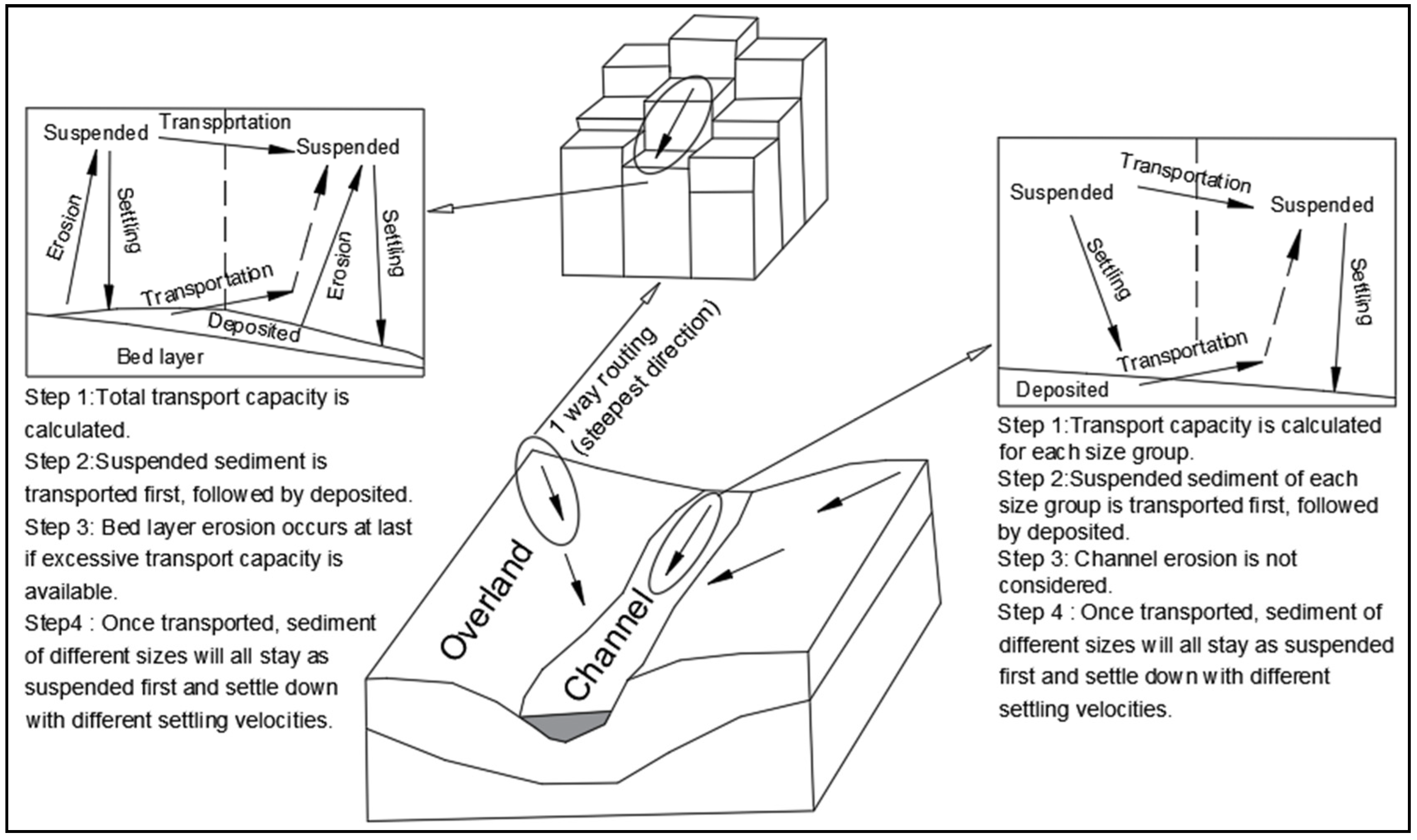
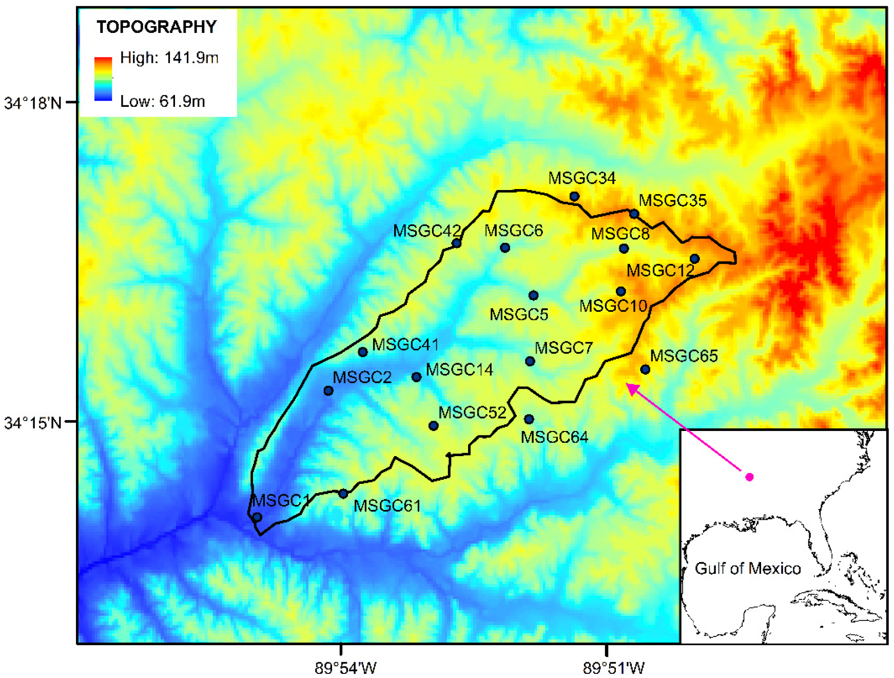
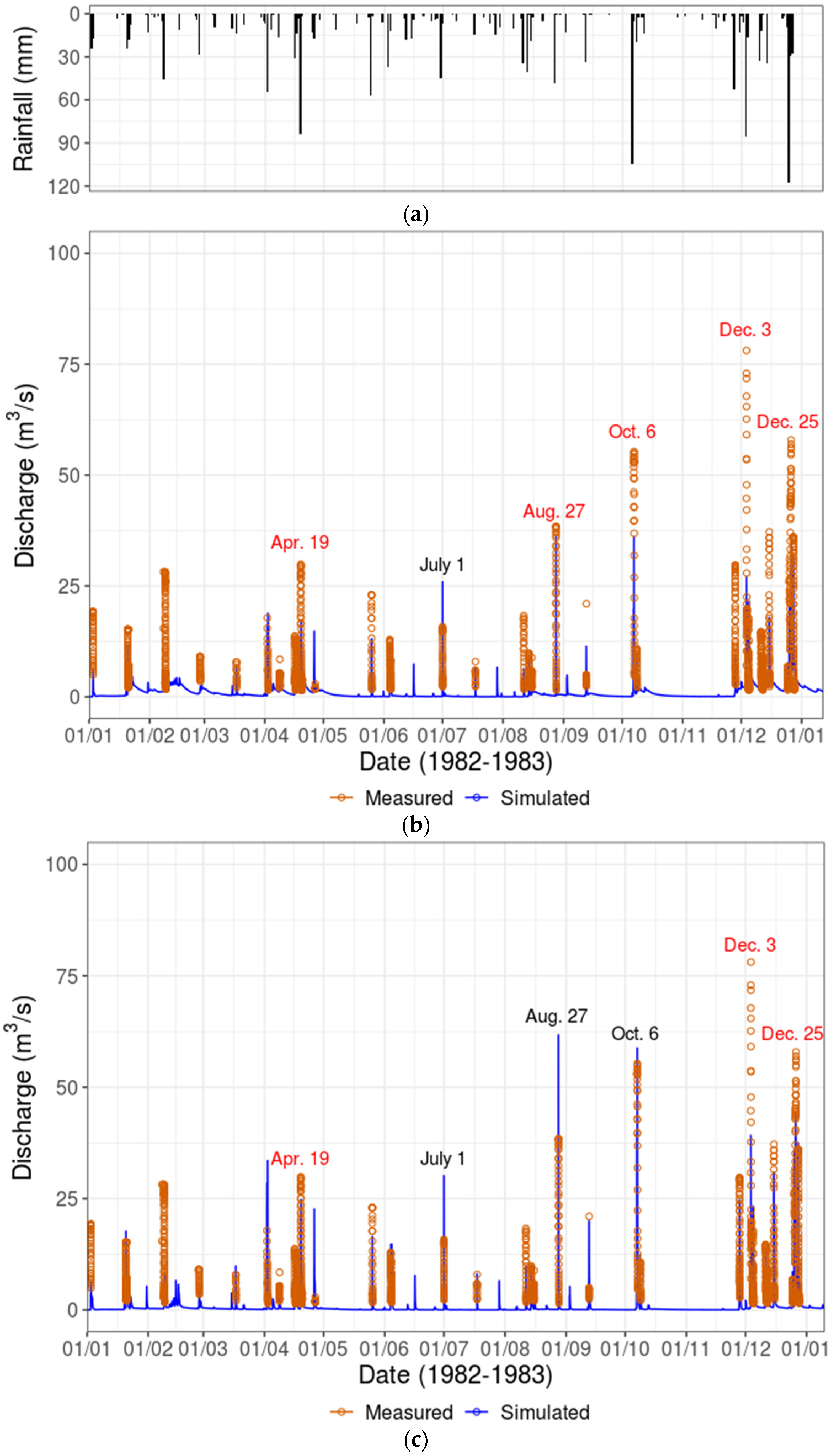
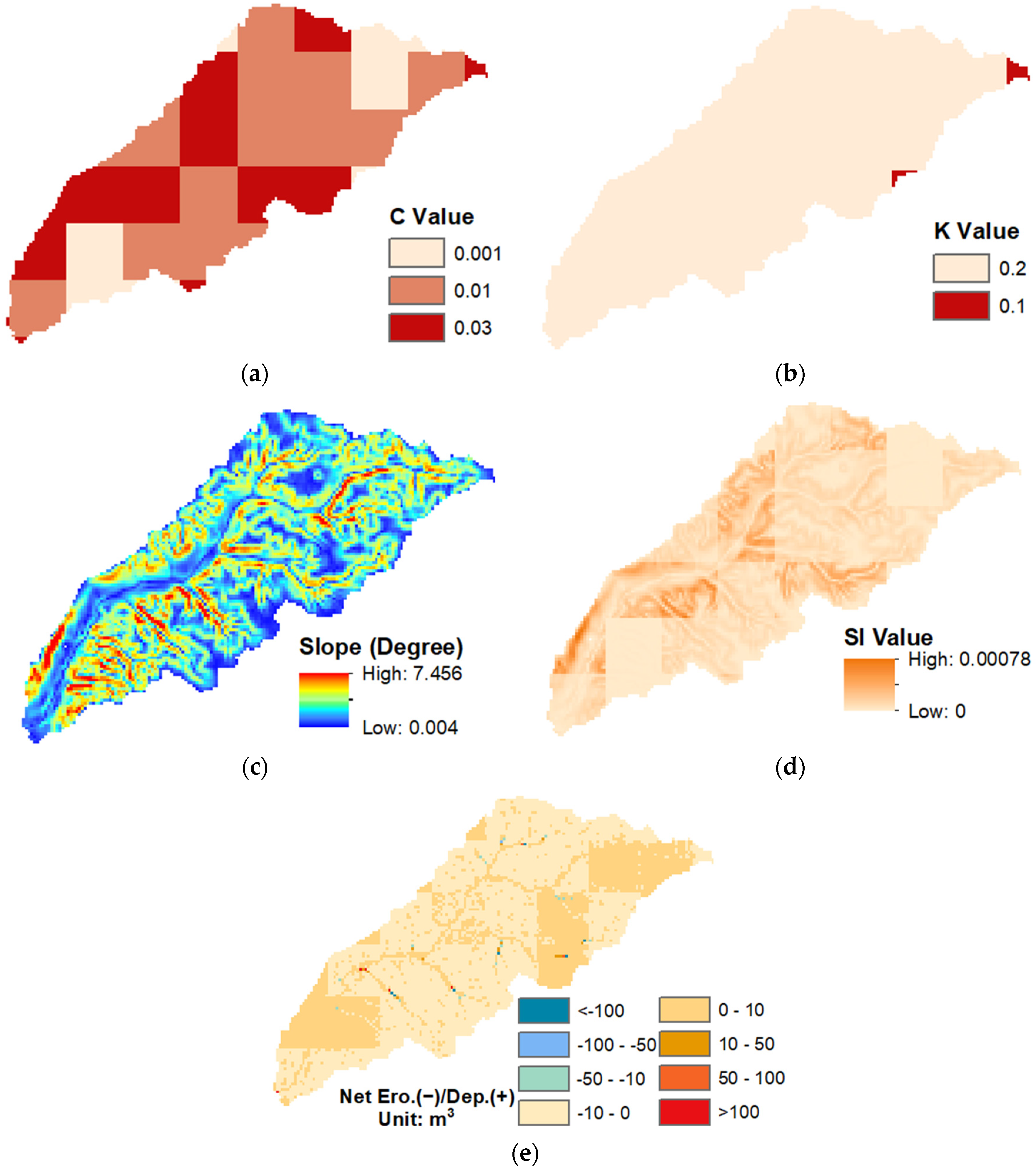
In this study, by adapting the sediment algorithm from CASC2D-Sed, we introduced a sediment module into the WRF-Hydro platform, allowing for the development of a fully distributed, process-based soil erosion and sediment transport model (WRF-Hydro-Sed). The model’s performance was evaluated via a comparison with the observed streamflow and sediment concentration data at the Goodwin Creek Experimental Watershed during rainfall events.
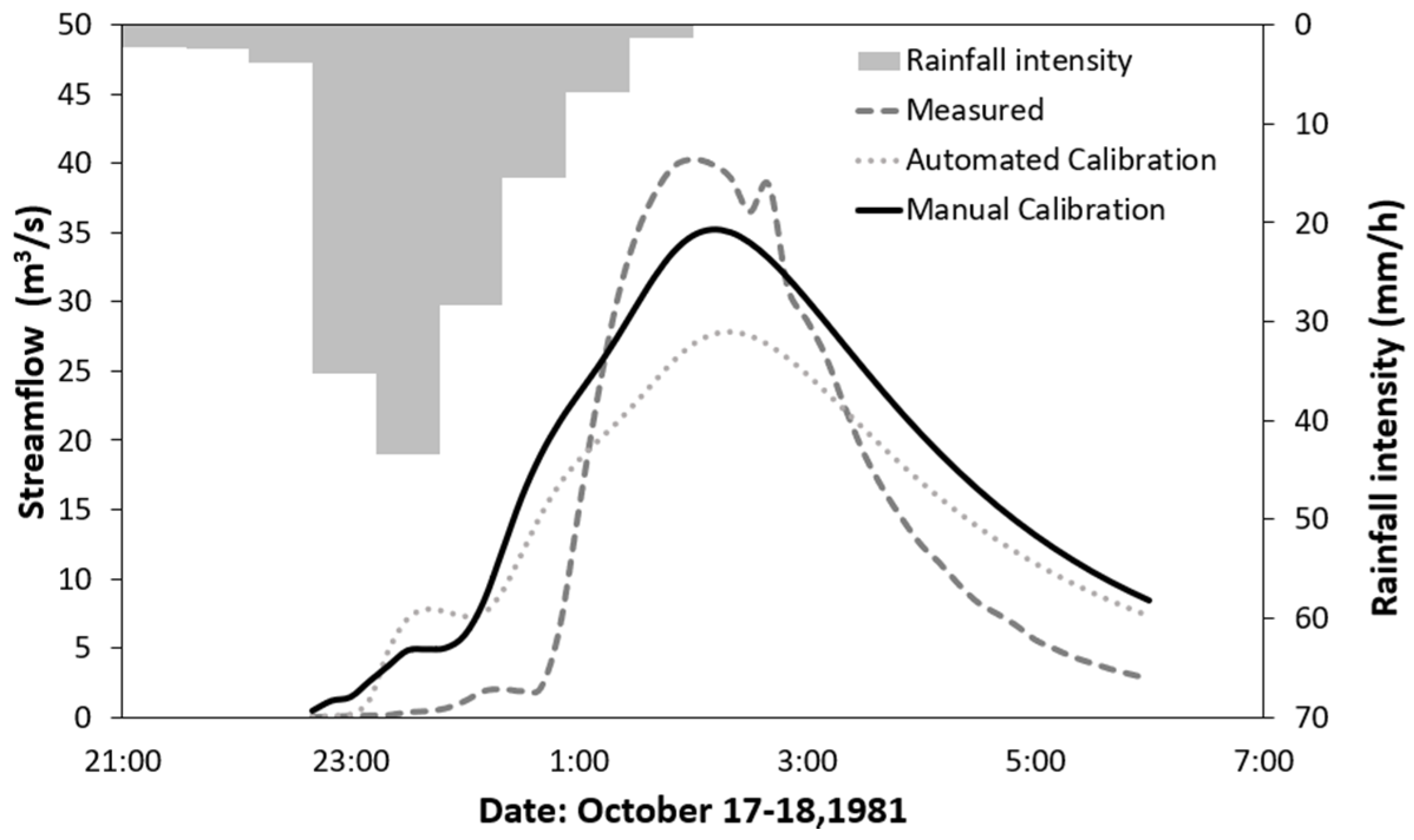
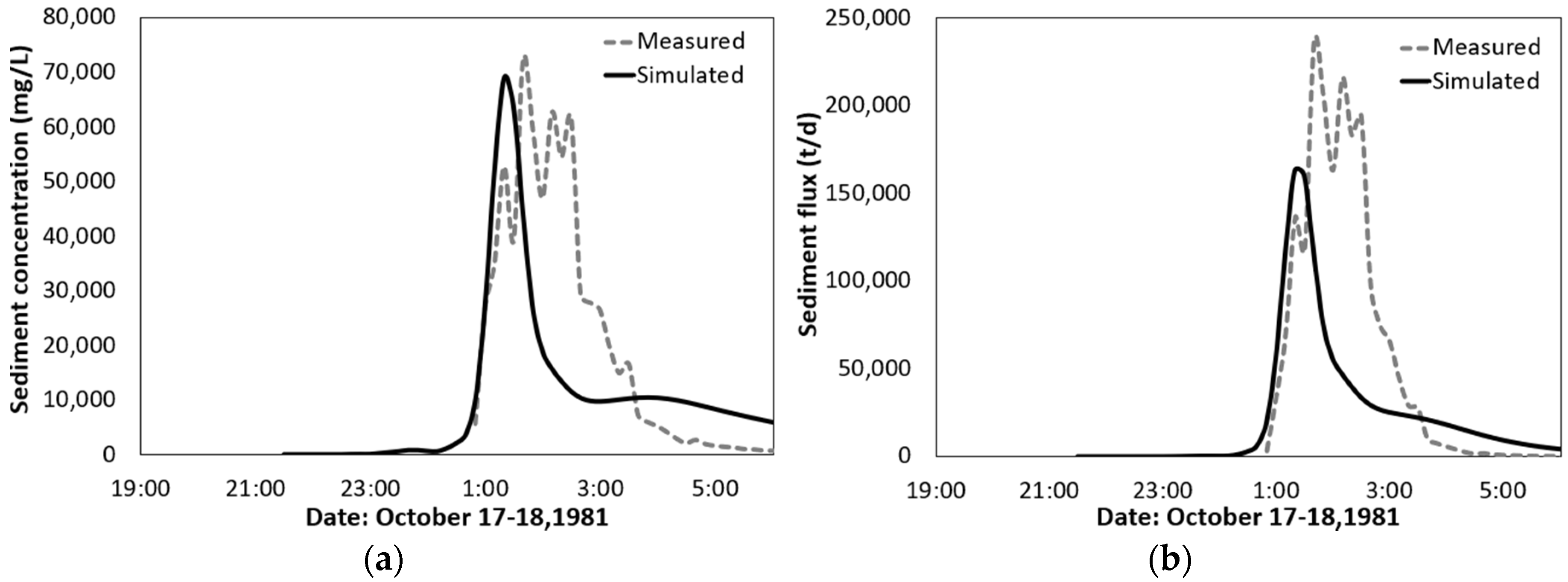
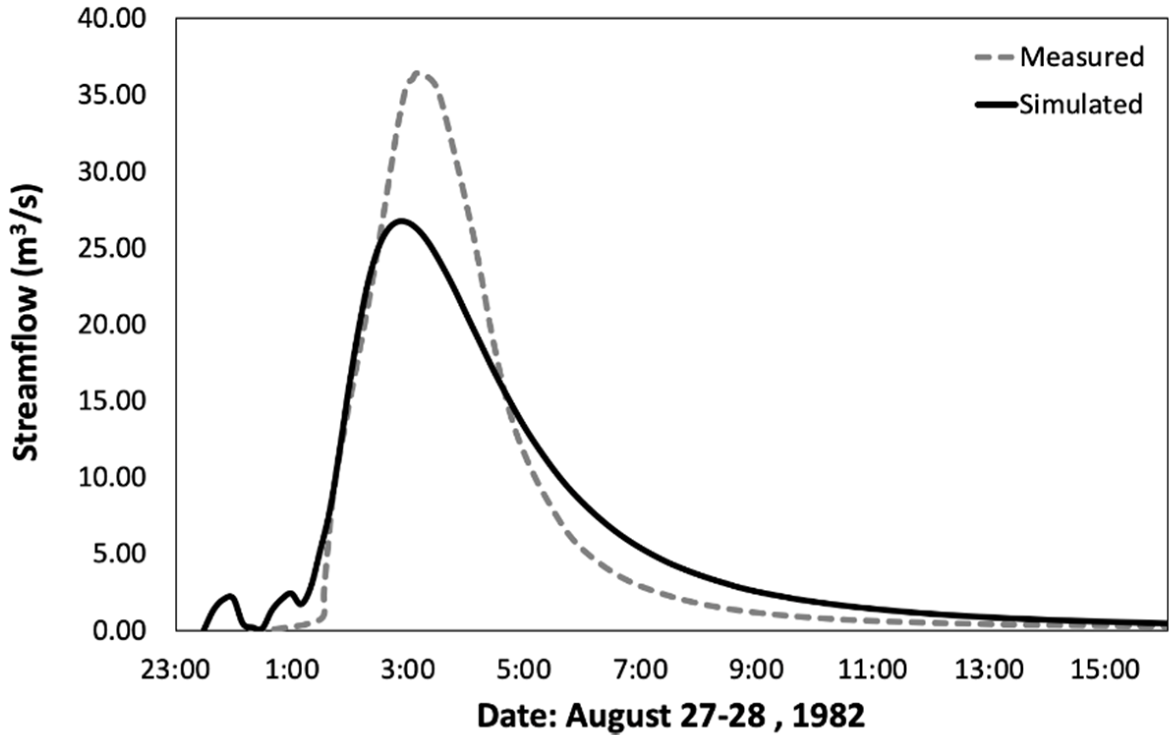
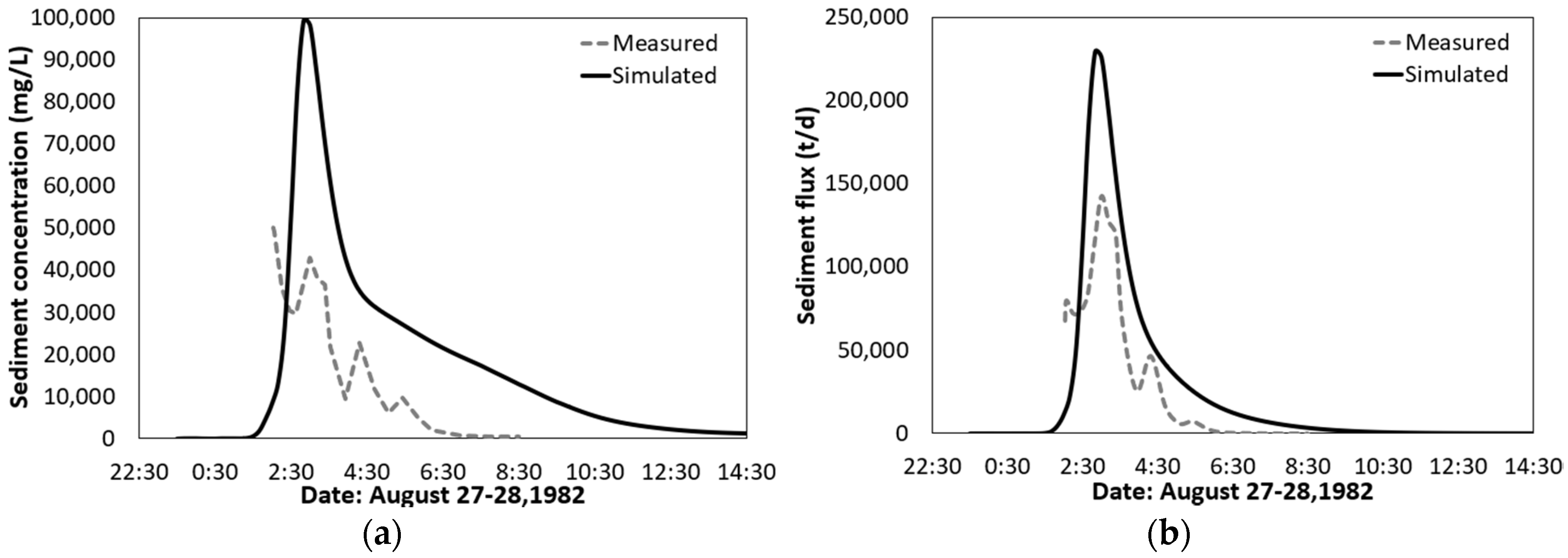
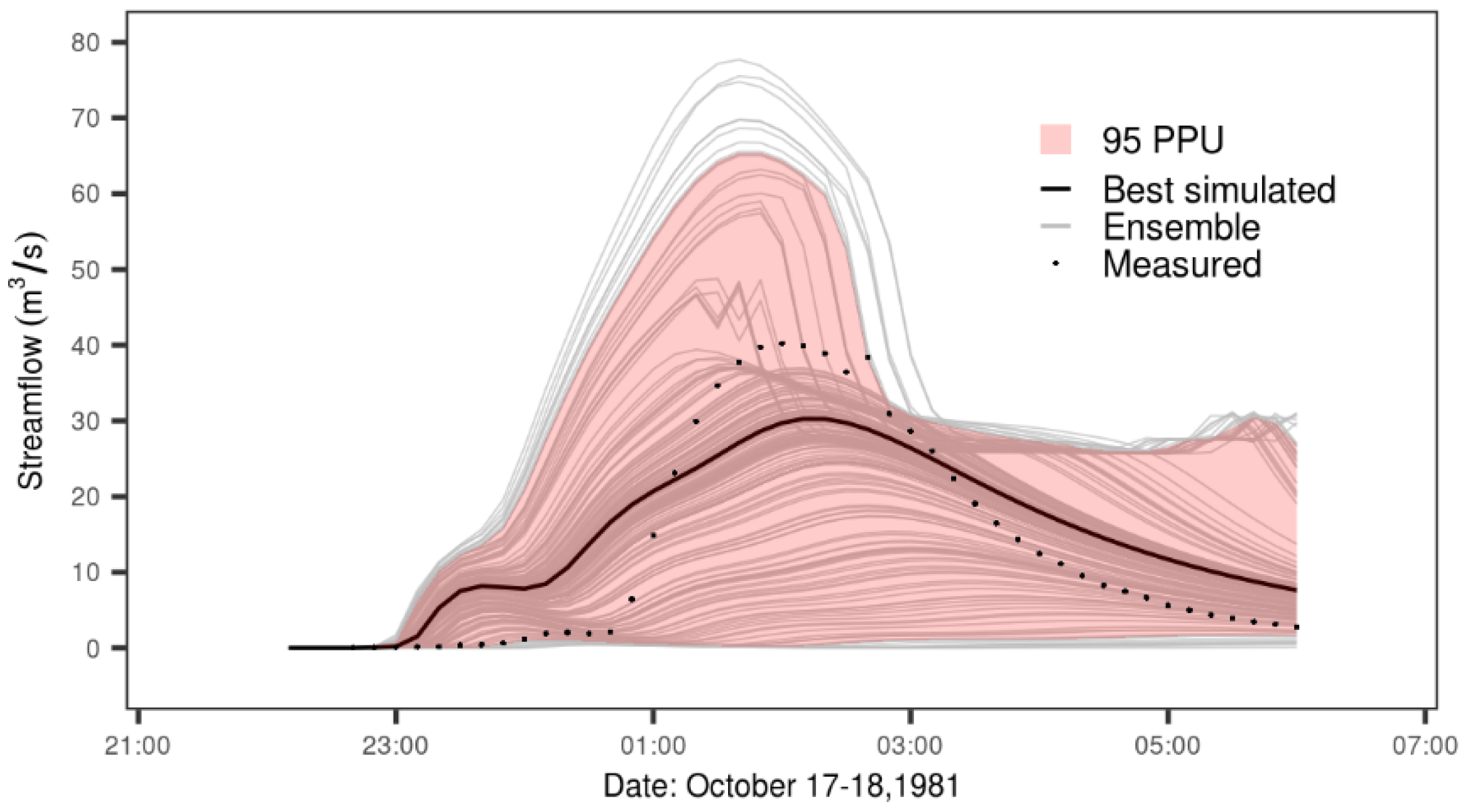
WRF-Hydro-Sed is able to generate satisfactory results of streamflow and sediment yield during rainfall events. The streamflow can be calibrated successfully based on a single rainfall event with the adjustment of a few hydro-parameters including refkdt (the parameter that controls runoff–infiltration partition) and channel geometries. With the single event calibrated hydro-parameters, the model can also perform satisfactorily in simulating the hydrograph during a validation event. Based on calibrated hydro-parameters, sediment concentration, sediment flux, as well as sediment yield can also be calibrated successfully at watershed scale by adjusting sediment parameters related to land use and soil category. Satisfactory results are also generated for a validation event using calibrated sediment parameters. The model’s performance in simulating sediment yield is better than sediment concentration and flux.
The model’s performance in streamflow simulation is sensitive to forcing data. The original NLDAS-2, given its 1/8 degree coarse resolution, may not be an optimal choice to provide rainfall forcing for simulation over a relatively small watershed like the Goodwin Creek under local storm events. High resolution meteorological forcing data is recommended for application of the WRF-Hydro-Sed on a small watershed.
Calibrated hydro-parameters based on a single event can be applied to different rainfall events to reproduce the hydrograph. While it might not be practical to have a set of parameters that can be suitable for any rainfall event, an intensive calibration based on multiple events can improve the model’s performance to a certain degree, but with extensive computational efforts. In this case, intensive calibration over a long time scale might not be an optimal strategy if computational cost is a major concern and if the model performance based on a single event calibration is acceptable. With the calibrated sediment parameters based on a single event, the sediment yield over different events can be simulated within the same magnitude observed. Moreover, the model shows promising potential in simulating annual soil erosion on a watershed scale. While simulated sediment yield is considered acceptable for 71% of the events (12 out of 17), substantial bias can be found during certain events mainly due to the bias transferred from the streamflow simulation. Future development of the model by including the bank and channel erosion algorithm is expected to further improve model performance.

Supplementary Materials

The following are available online at https://www.mdpi.com/2073-4441/12/6/1840/s1, the equations used to calculate correlation coefficient, RMSE, NSE and KGE.

Author Contributions

Conceptualization, Z.G.X. and D.Y.; methodology, D.Y.; software, D.Y. and W.Y.; validation, D.Y.; formal analysis, D.Y. and M.M.; investigation, D.Y. and M.M.; resources, Z.G.X. and D.J.G.; data curation, D.Y.; writing—original draft preparation, D.Y.; writing—review and editing, D.Y., Z.G.X. and A.R.; visualization, D.Y. and Z.G.X.; supervision, Z.G.X.; project administration, Z.G.X. and D.J.G.; funding acquisition, Z.G.X. and D.J.G. All authors have read and agreed to the published version of the manuscript.

Funding

This project was funded by The Water Institute of the Gulf under project “Project Louisiana Rivers’ Sediment Flux to the Coastal Ocean using a Coupled Atmospheric-Hydrological Model” (award number RCEGR260003-01-00). This project was paid for (in part) with federal funding from the Department of the Treasury through the Louisiana Coastal Protection and Restoration Authority’s Center of Excellence Research Grants Program under the Resources and Ecosystems Sustainability, Tourist Opportunities, and Revived Economies of the Gulf Coast States Act of 2012 (RESTORE Act). The statements, findings, conclusions, and recommendations are those of the author(s) and do not necessarily reflect the views of the Department of the Treasury, CPRA or The Water Institute of the Gulf. Dongxiao Yin is also supported by the Economic Development Assistantship program at LSU. Support from NCAR’s Advanced Study Program’s Graduate Student (GVP) Fellowship is appreciated. This research is also partially funded by USGS The Cooperative Ecosystem Studies Units (award# G20AC00099).

Acknowledgments

Louisiana Optical Network Initiative (LONI), and Cheyenne (doi: 10.5065/D6RX99HX) provided by NCAR’s Computational and Information Systems Laboratory, sponsored by the National Science Foundation are acknowledged for high-performance computing support. We acknowledge the NCAR WRF-Hydro developing team for help with model setup. Glenn V. Wilson and Jacob Ferguson are thanked for providing us with the data of GCEW.

Conflicts of Interest

The authors declare no conflict of interest.

References

  1. Amundson, R.; Berhe, A.A.; Hopmans, J.W.; Olson, C.; Sztein, A.E.; Sparks, D.L. Soil and human security in the 21st century. Science 2015, 348. [Google Scholar] [CrossRef] [Green Version]
  2. Juez, C.; Tena, A.; Fernández-Pato, J.; Batalla, R.J.; García-Navarro, P. Application of a distributed 2D overland flow model for rainfall/runoff and erosion simulation in a Mediterranean watershed. Geogr. Res. Lett. 2018, 44, 615–640. [Google Scholar] [CrossRef] [Green Version]
  3. Aksoy, H.; Kavvas, M.L. A review of hillslope and watershed scale erosion and sediment transport models. Catena 2005, 64, 247–271. [Google Scholar] [CrossRef]
  4. Fatichi, S.; Vivoni, E.R.; Ogden, F.L.; Ivanov, V.Y.; Mirus, B.; Gochis, D.; Downer, C.W.; Camporese, M.; Davison, J.H.; Ebel, B.; et al. An overview of current applications, challenges, and future trends in distributed process-based models in hydrology. J. Hydrol. 2016, 537, 45–60. [Google Scholar] [CrossRef] [Green Version]
  5. Knisel, W.G. CREAMS A Field-Scale Model for Chemicals, Runoff, and Erosion from Agricultural Management Systems; Science and Education Administration: Washington, WA, USA, 1982. [Google Scholar]
  6. Nearing, M.A.; Foster, G.R.; Lane, L.J.; Finkner, S.C. A Process-based soil erosion model for USDA-water erosion prediction project technology. Trans. ASAE 1989, 32, 1587–1593. [Google Scholar] [CrossRef]
  7. Morgan, R.P.C.; Quinton, J.N.; Smith, R.E.; Govers, G.; Poesen, J.W.A.; Auerswald, K.; Chisci, G.; Torri, D.; Styczen, M.E. The European soil erosion model (EUROSEM): A dynamic approach for predicting sediment transport from fields and small catchments. Earth Surf. Process. Landf. 1998, 23, 527–544. [Google Scholar] [CrossRef]
  8. Smith, R.E. A kinematic model for surface mine sediment yield. Trans. Am. Soc. Agric. Eng. 1981, 24, 1508–1514. [Google Scholar] [CrossRef]
  9. Patil, S.; Sivapalan, M.; Hassan, M.A.; Ye, S.; Harman, C.J.; Xu, X. A network model for prediction and diagnosis of sediment dynamics at the watershed scale. J. Geophys. Res. Earth Surf. 2012, 117, 1–17. [Google Scholar] [CrossRef] [Green Version]
  10. Merritt, W.S.; Letcher, R.A.; Jakeman, A.J. A review of erosion and sediment transport models. Environ. Model. Softw. 2003, 18, 761–799. [Google Scholar] [CrossRef]
  11. De Roo, A.P.J.; Wesseling, C.G.; Ritsema, C.J. LISEM: A Single-event physically based hydrological and soil erosion model for drainage basins. I: Theory, input and output. Hydrol. Process. 1996, 10, 1107–1117. [Google Scholar] [CrossRef]
  12. Wicks, J.M.; Bathurst, J.C. SHESED: A physically based, distributed erosion and sediment yield component for the SHE hydrological modelling system. J. Hydrol. 1996, 175, 213–238. [Google Scholar] [CrossRef]
  13. Johnson, B.E.; Julien, P.Y.; Molnar, D.K.; Watson, C.C. The two-dimensional upland erosion model CASC2D-SED. J. Am. Water Resour. Assoc. 2000, 36, 31–42. [Google Scholar] [CrossRef]
  14. Juez, C.; Battisacco, E.; Schleiss, A.J.; Franca, M.J. Assessment of the performance of numerical modeling in reproducing a replenishment of sediments in a water-worked channel. Adv. Water Resour. 2016, 92, 10–22. [Google Scholar] [CrossRef]
  15. Gochis, D.J.; Yu, W.; Yates, D. The WRF-Hydro model technical description and user’s guide, Version 3.0. NCAR Tech. Doc. 2015, 120. [Google Scholar] [CrossRef]
  16. Liang, X.; Lettenmaier, D.P.; Wood, E.F.; Burges, S.J. A simple hydrologically based model of land surface water and energy fluxes for general circulation models. J. Geophys. Res. 1994, 99, 14415–14428. [Google Scholar] [CrossRef]
  17. Arnold, J.G.; Srinivasan, R.; Muttiah, R.S.; Williams, J.R. Large area hydrologic modeling and assessment. Part I: Model development. Nutrition 1998, 17, 70. [Google Scholar] [CrossRef]
  18. Lin, P.; Hopper, L.J.; Yang, Z.-L.; Lenz, M.; Zeitler, J.W. Insights into hydrometeorological factors constraining flood prediction skill during the May and October 2015 Texas Hill country flood events. J. Hydrometeorol. 2018, 19, 1339–1361. [Google Scholar] [CrossRef]
  19. Naabil, E.; Lamptey, B.L.; Arnault, J.; Kunstmann, H.; Olufayo, A. Water resources management using the WRF-Hydro modelling system: Case-study of the Tono dam in West Africa. J. Hydrol. Reg. Stud. 2017, 12, 196–209. [Google Scholar] [CrossRef]
  20. Somos-Valenzuela, M.A.; Palmer, R.N. Use of WRF-hydro over the Northeast of the US to estimate water budget tendencies in small watersheds. Water (Switz.) 2018, 10, 1709. [Google Scholar] [CrossRef] [Green Version]
  21. Xue, Z.G.; Gochis, D.J.; Yu, W.; Keim, B.D.; Rohli, R.V.; Zang, Z.; Sampson, K.; Dugger, A.; Sathiaraj, D.; Ge, Q. Modeling hydroclimatic change in Southwest Louisiana rivers. Water (Switz.) 2018, 10, 596. [Google Scholar] [CrossRef] [Green Version]
  22. Rojas, R.; Velleux, M.; Julien, P.Y.; Johnson, B.E. Grid scale effects on watershed soil erosion models. J. Hydrol. Eng. 2008, 13, 793–802. [Google Scholar] [CrossRef] [Green Version]
  23. Rojas Sánchez, R. GIS-Based Upland Erosion Modeling, Geovisualization and Grid Size Effects on Erosion Simulations with Casc2D-Sed. Ph.D. Thesis, Colorado State University, Fort Collins, CO, USA, 2002. [Google Scholar]
  24. Engelund, F.; Hansen, E. A Monograph on Sediment Transport in Alluvial Streams; Teknisk Forlag: Copenhagen, Denmark, 1967. [Google Scholar]
  25. Miller, D.A.; White, R.A. A Conterminous United States multilayer soil characteristics dataset for regional climate and hydrology modeling. Earth Interact. 1998, 2, 2. [Google Scholar] [CrossRef]
  26. McKay, L.; Bondelid, T.; Dewald, T.; Johnston, J.; Moore, R.; Rea, A. NHDPlus Version 2: User Guide. 2012, p. 182. Available online: ftp://ftp.horizon-systems.com/NHDplus/NHDPlusV21/Documentation/NHDPlusV2_User_Guide.pdf (accessed on 26 June 2020).
  27. Niu, G.Y.; Yang, Z.L.; Mitchell, K.E.; Chen, F.; Ek, M.B.; Barlage, M.; Kumar, A.; Manning, K.; Niyogi, D.; Rosero, E.; et al. The community Noah land surface model with multiparameterization options (Noah-MP): 1. Model description and evaluation with local-scale measurements. J. Geophys. Res. Atmos. 2011, 116, 1–19. [Google Scholar] [CrossRef] [Green Version]
  28. Sertel, E.; Robock, A.; Ormeci, C. Impacts of land cover data quality on regional climate simulations. Int. J. Climatol. 2010, 30, 1942–1953. [Google Scholar] [CrossRef]
  29. Xia, Y.; Mitchell, K.; Ek, M.; Sheffield, J.; Cosgrove, B.; Wood, E.; Luo, L.; Alonge, C.; Wei, H.; Meng, J.; et al. Continental-scale water and energy flux analysis and validation for the North American Land Data Assimilation System project phase 2 (NLDAS-2): 1. Intercomparison and application of model products. J. Geophys. Res. Atmos. 2012, 117, D03110. [Google Scholar] [CrossRef]
  30. Tolson, B.A.; Shoemaker, C.A. Dynamically dimensioned search algorithm for computationally efficient watershed model calibration. Water Resour. Res. 2007, 43, 1–16. [Google Scholar] [CrossRef]
  31. Arnault, J.; Wagner, S.; Rummler, T.; Fersch, B.; Bliefernicht, J.; Andresen, S.; Kunstmann, H. Role of runoff-infiltration partitioning and resolved overland flow on land-atmosphere feedbacks: A case study with the WRF-hydro coupled modeling system for West Africa. J. Hydrometeorol. 2016, 17, 1489–1516. [Google Scholar] [CrossRef]
  32. Yucel, I.; Onen, A.; Yilmaz, K.K.; Gochis, D.J. Calibration and evaluation of a flood forecasting system: Utility of numerical weather prediction model, data assimilation and satellite-based rainfall. J. Hydrol. 2015, 523, 49–66. [Google Scholar] [CrossRef] [Green Version]
  33. Ehret, U.; Zehe, E. Series distance—An intuitive metric to quantify hydrograph similarity in terms of occurrence, amplitude and timing of hydrological events. Hydrol. Earth Syst. Sci. 2011, 15, 877–896. [Google Scholar] [CrossRef] [Green Version]
  34. Julien, P.Y. Erosion and Sedimentation, 2nd ed.; Cambridge University Press: Cambridge, UK, 2010. [Google Scholar]
  35. Elliott, A.H.; Oehler, F.; Schmidt, J.; Ekanayake, J.C. Sediment modelling with fine temporal and spatial resolution for a hilly catchment. Hydrol. Process. 2012, 26, 3645–3660. [Google Scholar] [CrossRef]
  36. Fufa, S.D.; Strauss, P.; Schneider, W. Comparison of erodibility of some Hararghe soils using rainfall simulation. Commun. Soil Sci. Plant Anal. 2002, 33, 333–348. [Google Scholar] [CrossRef]
  37. Vergara, H.; Hong, Y.; Gourley, J.J.; Anagnostou, E.N.; Maggioni, V.; Stampoulis, D.; Kirstetter, P.-E. Effects of resolution of satellite-based rainfall estimates on hydrologic modeling skill at different scales. J. Hydrometeorol. 2013, 15, 593–613. [Google Scholar] [CrossRef] [Green Version]
  38. Setegn, S.G.; Srinivasan, R.; Melesse, A.M.; Dargahi, B. SWAT model application and prediction uncertainty analysis in the Lake Tana Basin, Ethiopia. Hydrol. Process. 2009, 24, 357–367. [Google Scholar] [CrossRef]
  39. Rafiei Emam, A.; Kappas, M.; Fassnacht, S.; Linh, N.H.K. Uncertainty analysis of hydrological modeling in a tropical area using different algorithms. Front. Earth Sci. 2018, 12, 661–671. [Google Scholar] [CrossRef]
  40. Wu, H.; Chen, B. Evaluating uncertainty estimates in distributed hydrological modeling for the Wenjing River watershed in China by GLUE, SUFI-2, and ParaSol methods. Ecol. Eng. 2015, 76, 110–121. [Google Scholar] [CrossRef]
  41. Yang, J.; Reichert, P.; Abbaspour, K.C.; Xia, J.; Yang, H. Comparing uncertainty analysis techniques for a SWAT application to the Chaohe Basin in China. J. Hydrol. 2008, 358, 1–23. [Google Scholar] [CrossRef]
  42. Kim, J.; Ivanov, V.Y.; Katopodes, N.D. Modeling erosion and sedimentation coupled with hydrological and overland flow processes at the watershed scale. Water Resour. Res. 2013, 49, 5134–5154. [Google Scholar] [CrossRef]
  43. Moriasi, D.N.; Arnold, J.G.; Van Liew, M.W.; Bingner, R.L.; Harmel, R.D.; Veith, T.L. Model evaluation guidelines for systematic quantification of accuracy in watershed simulations. Trans. ASABE 2007, 50, 885–900. [Google Scholar] [CrossRef]
  44. Jia, Y.; Tang, L.; Xu, M.; Yang, X. Landscape pattern indices for evaluating urban spatial morphology—A case study of Chinese cities. Ecol. Indic. 2019, 99, 27–37. [Google Scholar] [CrossRef]
  45. Ahmadi Mirghaed, F.; Souri, B.; Mohammadzadeh, M.; Salmanmahiny, A.; Mirkarimi, S.H. Evaluation of the relationship between soil erosion and landscape metrics across Gorgan Watershed in northern Iran. Environ. Monit. Assess. 2018, 190, 643. [Google Scholar] [CrossRef]
  46. Ouyang, W.; Skidmore, A.K.; Hao, F.; Wang, T. Soil erosion dynamics response to landscape pattern. Sci. Total Environ. 2010, 408, 1358–1366. [Google Scholar] [CrossRef] [PubMed]
  47. Zhou, Z.X.; Li, J. The correlation analysis on the landscape pattern index and hydrological processes in the Yanhe watershed, China. J. Hydrol. 2015, 524, 417–426. [Google Scholar] [CrossRef]
  48. Routschek, A.; Schmidt, J.; Kreienkamp, F. Impact of climate change on soil erosion—A high-resolution projection on catchment scale until 2100 in Saxony/Germany. Catena 2014, 121, 99–109. [Google Scholar] [CrossRef]
  49. Mullan, D.; Favis-Mortlock, D.; Fealy, R. Addressing key limitations associated with modelling soil erosion under the impacts of future climate change. Agric. For. Meteorol. 2012, 156, 18–30. [Google Scholar] [CrossRef] [Green Version]
  50. Kuhnle, R.A.; Bingner, R.L.; Foster, G.R.; Grissinger, E.H. Effect of land use changes on sediment transport. Water Resour. Res. 1996, 32, 3189–3196. [Google Scholar] [CrossRef]
Figure 1. Schematic structure of WRF-Hydro-Sed.
Water 12 01840 g001
Figure 2. Schematic representation of WRF-Hydro-Sed.
Water 12 01840 g002
Figure 3. Topography of Goodwin Creek Experimental Watershed (GCEW) and gage location (DEM data source: National Hydrography Dataset Plus (Version 2), [26]).
Water 12 01840 g003
Figure 4. Measured (dash line), manually calibrated (solid line) and automatically calibrated (dot line) streamflow at MSGC01 for calibration event. Time series of rainfall intensity is also shown.
Water 12 01840 g004
Figure 5. Measured (dash line) and simulated (solid line) sediment concentration (a), and sediment flux (b) at MSGC01 for calibration event.
Water 12 01840 g005
Figure 6. Measured (dash line) and simulated (solid line) streamflow at MSGC01 for validation event.
Water 12 01840 g006
Figure 7. Measured (dash line) and simulated (solid line) sediment concentration (a), and sediment flux (b) at MSGC01 for validation event.
Water 12 01840 g007
Figure 8. Measured (dash line) and simulated hydrographs (solid line for updated NLDAS-2, dash-dotted line for original NLDAS-2) at MSGC01 for calibration event.
Water 12 01840 g008
Figure 9. The best-simulated streamflow with 95 PPU and observations during the calibration event in 17–18 October 1981.
Water 12 01840 g009
Figure 10. (a) Daily rainfall (black) of 1982. (b) Measured (dark orange) and simulated (blue, based on calibrated hydro-parameters) hydrographs at MSGC01 for all the rainfall events of 1982. (c) Same as (b) but based on recalibrated hydro-parameters. Several rainfall events are annotated with red, indicating underestimation and black represents overestimation.
Water 12 01840 g010
Figure 11. C value (a), K value (b), slope (c), and SI (d) over GCEW, and Net Erosion ()/Deposition (+) (e) during calibration event over GCEW.
Water 12 01840 g011
Table 1. Calibrated hydro-parameters using the NCAR developed calibration tool.
ParameterValuesDescription
MinMaxInitial
bexp0.41.91.0Multiplier on pore size distribution index
smcmax0.81.21.0Multiplier on saturation soil moisture content
dksat0.2101.0Multiplier on saturated soil hydraulic conductivity
refkdt0.141.0Surface runoff parameter
slope010.3Linear scaling of “openness” of bottom drainage boundary
RETDEPRTFAC0.120,0001.0Multiplier on maximum retention depth before flow is routed as overland flow.
LKSATFAC1010,0001000Multiplier on saturated hydraulic conductivity in lateral flow direction
cwpvt0.521.0Multiplier on canopy wind parameter
vcmx250.61.41.0Multiplier on maximum rate of carboxylation at 25 °C (umol CO2/m2/s)
Table 2. Calibrated sediment parameters and values for sediment model.
Land Use CategoryCPSoil TypeK (t/Acre)
Dryland cropland and pasture0.010.1Silt loam0.2
Irrigated cropland and pasture0.030.1Sandy loam0.1
Deciduous broadleaf forest0.0010.1
Table 3. Performance of the streamflow simulation for calibration event.
LocationCalibration MethodsCorrelation CoefficientRMSE (m3/s)NSEKGE
MSGC01 (Outlet)Automated0.937.210.740.57
Manual0.946.720.770.63
Table 4. Values of manually calibrated hydro-parameters.
ParameterValueParameterValue
refkdt0.7Chsslp1st order channel0.35
RETDEPRTFAC1.02nd order channel0.25
Bw1st order channel3.0MannN1st order channel0.35
2nd order channel5.02nd order channel0.15
Table 5. Performance of the simulation of sediment concentration and sediment flux for calibration event.
LocationVariableCorrelation CoefficientRMSENSEKGE
MSGC01 (Outlet)Sediment concentration0.5719,692.64 mg/L0.250.44
Sediment flux0.6265,321.10 t/d0.280.30
Table 6. Performance of the simulation of streamflow, sediment concentration, and sediment flux for validation event.
LocationVariableCorrelation CoefficientRMSENSEKGE
MSGC01 (Outlet)Streamflow0.975.09 m3/s0.860.70
Sediment concentration0.4330,541.63 mg/L−2.26−0.15
Sediment flux0.8544,922.10 t/d0.090.34
Table 7. Rainfall intensity, duration, and return period, simulated and observed sediment yield for 17 sediment events during 1982. Sediment events of 3–4 June, 3–4 December, and 24–28 December include 3, 2 and 3 rainfall events, respectively. Return period < 1 represents normal rainfall event.
DateRainfall Intensity (mm/h)Duration (h)Return Period (years)Sediment Yield (t)
MeasuredSimulatedMeasured/Simulated
2–3 January4.15<1156617380.90
8 February5.36.5790337112.13
8 April3.641333740.36
17 April3.84.59691775.47
19 April4.29677711,6500.58
25 May10.62.5268419,8930.13
3–4 June8.481533433,6850.16
1.91.5<1
6.02
11 August5.66<144038055.47
14 August5.55205446410.44
15 August2.96.51801681.07
6–7 October9.011.5734,99657,7690.61
8 October6.23<1301940710.74
27 November3.714892386121.04
3–4 December4.121~148,38025,9321.87
3.15<1
10–11 December1.529<1598415963.75
15 December3.98.5984295691.03
24–28 December5.81.5<160,24044,3071.36
4.3346
4.97.5<1
Sum 203,387228,6980.89

