Numerical 3D Model Development and Validation of Curb-Cut Inlet for Efficiency Prediction

Abstract

Green infrastructure (GI) is a decentralized stormwater management strategy that can simultaneously enhance the resilience of the urban landscape to weather-related stressors. The effectiveness of individual GI facilities is determined by the physical characteristics of the tributary area and inlet, including factors such as slope and geometry, apron configuration, roughness, and clogging, all of which have been inadequately studied. In this paper, we construct, calibrate, and validate a computational fluid dynamics (CFD) model using field survey data collected at a Bronx, NY GI facility. The validated CFD model is used to evaluate how inlet clogging and flow rate affect GI inlet performance. Seven flow rates ranging from 0.00044 to 0.00755 CMS were simulated. As the flow rate increased, the inlet efficiency dropped from 100% to 60% at one location (the SW inlet) and from 100% to 25% at another location (the NW inlet). At a fixed flow rate, the inlet efficiency dropped from 100% efficient (with no clogging) to 0% (with the inlet fully clogged). The stage-discharge relationship for the inlet based on the simulated field conditions deviated from that assumed based on normative flow and was revised. We suggest that GI facilities installed on mild- slope, or rough streets be fitted with non-clogging inlets to maintain free outfall conditions.

1. Introduction

As global urbanization reaches unprecedented levels, there is a need to plan, design, and update infrastructure systems in cities, including water infrastructure. Urban infrastructure is likely to face a significant increase in weather-related risks due to factors such as climate change [1]. Against this backdrop, urban designers have been increasingly looking to green infrastructure (GI) as a distributed way to retain and detain stormwater throughout an urban watershed. By slowing down the flow of runoff within the watershed, natural hydrologic processes such as infiltration, recharge, and evapotranspiration can be restored into the urban landscape, reducing the rate and volume of runoff (and associated pollutants) discharged to collection systems and the receiving water-bodies to which they drain.

An important question for urban drainage engineers is the rate at which runoff can be routed through engineered inlets into GI systems. Although tributary area characteristics such as pavement depression storage have been found to be important [2], inlets are also key determinants of GI performance. Inefficient or clogged inlets can cause localized street flooding [3] while underutilizing the engineered storage capacity of individual GI facilities [4]. To the extent that GI is a key part of the urban drainage planning, they are also critical drivers of the hydrologic performance of the entire urban watershed.

Though municipal GI programs are well underway, research to improve GI facility design is minimal. There has been extensive laboratory research focusing on highway stormwater inlets [5,6,7,8], but because their geometry differs from typical GI inlets, the transferability of these findings is limited. Additionally, most highway inlet research was conducted in laboratories under controlled conditions that are quite different from typical GI field conditions.

Flow through GI inlets can be modeled, though work in this area has also been minimal. Normative hydrologic and hydraulic (H&H) modeling tools used by urban drainage engineers—such as the stormwater management model—(SWMM) generally assume 100% efficient inlets [9]. However, field observations indicate that the momentum of the approaching flow tends to carry it past the inlet opening [6]. This discrepancy in observed and modeled inflow rates and volumes can result in inaccurate hydrologic mass balances, with implications on understanding of particulate matter transport [10] and other unit operations in the urban watershed.

In the US, where vertical curbs are common, GI facilities are often engineered into the sidewalk with flow into them passing through a “curb-cut,” often modeled as flow over a side weir. However, when water flows out of a channel over a side weirs it induces changes in flow pattern, velocity distribution, and mass transport in the main channel, e.g., gutter, [11] that make analytical solutions of the governing equations [12,13] difficult to solve. Some researchers have compared analytical solutions with laboratory experiments. Focusing on rectangular or trapezoidal weirs, Madjid Delkash and Babak Ebrazi Bakhshayesh [14], for example, modified DeMarchi’s equations derived from energy and momentum conservation to describe the flow regime. These equations, which utilize dimensionless parameters and the upstream Froude number to compute the coefficient of discharge, would need to be significantly modified to represent flow through actual GI inlet configurations, which have transverse bed slopes and are also subject to routine clogging.

With advances in computational capacity, researchers have recently begun using three-dimensional (3D) computational fluid dynamic (CFD) models to simulate inlet hydraulics as a cost-effective alternative to laboratory studies and analytical equations [15,16,17,18,19,20]. These researchers [9,18,20,21] have studied inlets, catch basins, and manholes with different geometries, using laboratory data for validation. CFD simulations of highway inlets suggest that upstream Froude number, flow rate, and profile (depth at various upstream locations), velocity and depth at the start of the inlet, and spread are the key physical determinants of inlet efficiency [13,22,23,24,25]. These studies prove that CFD models can be used to simulate a range of physical conditions and better understand the impact of physical conditions on specific flow processes, for example, the hydraulics of a GI inlet.

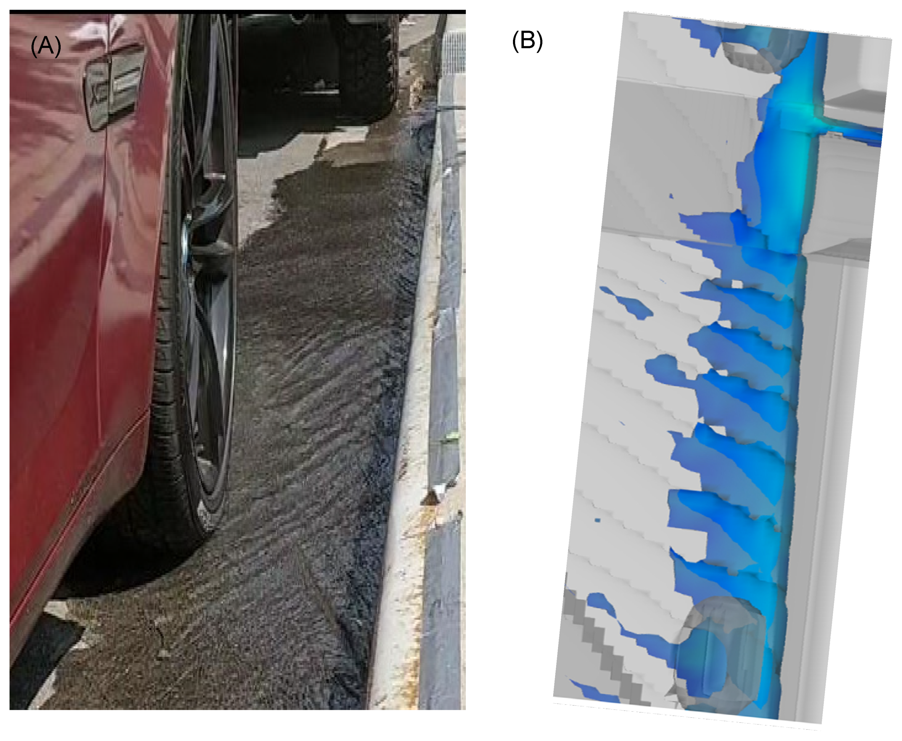
However, while CFD models can be useful in examining specific simulated flow processes in detail, a practical application of these studies requires real-world validation of the insights these models provide [10]. To date, CFD models are rarely compared to real-world experimental data. None of the above-mentioned studies utilized field observations in model (physical or CFD) construction, calibration, and validation. One advantage of field experiment data over laboratory experiments is that these observations include the full range of variability encountered in the real world. In the present context, field experiments can help study how actual morphological conditions of GI tributary areas and inlets, such as roughness, clogging, and as-built construction characteristics are related to inlet inflow and bypass.

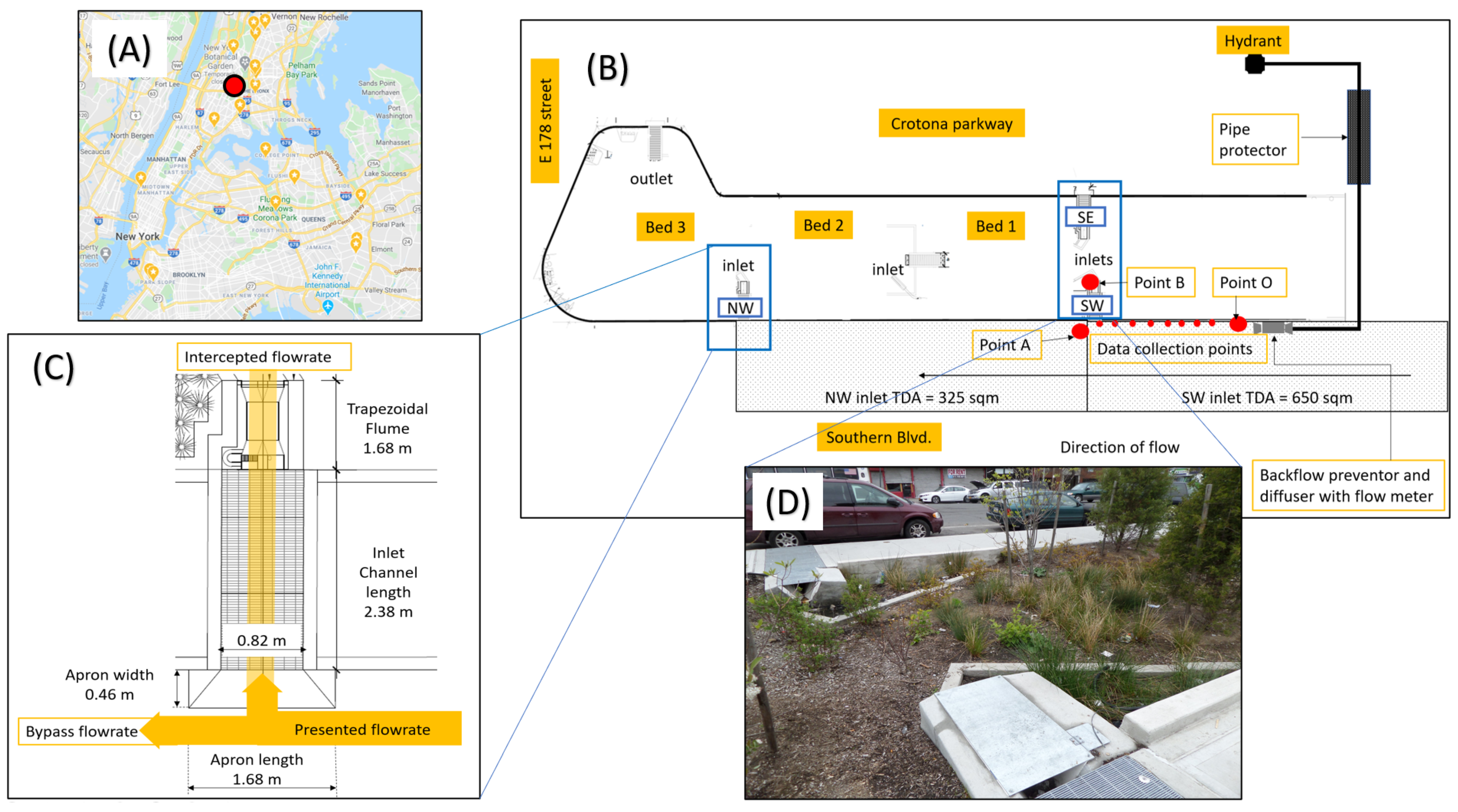
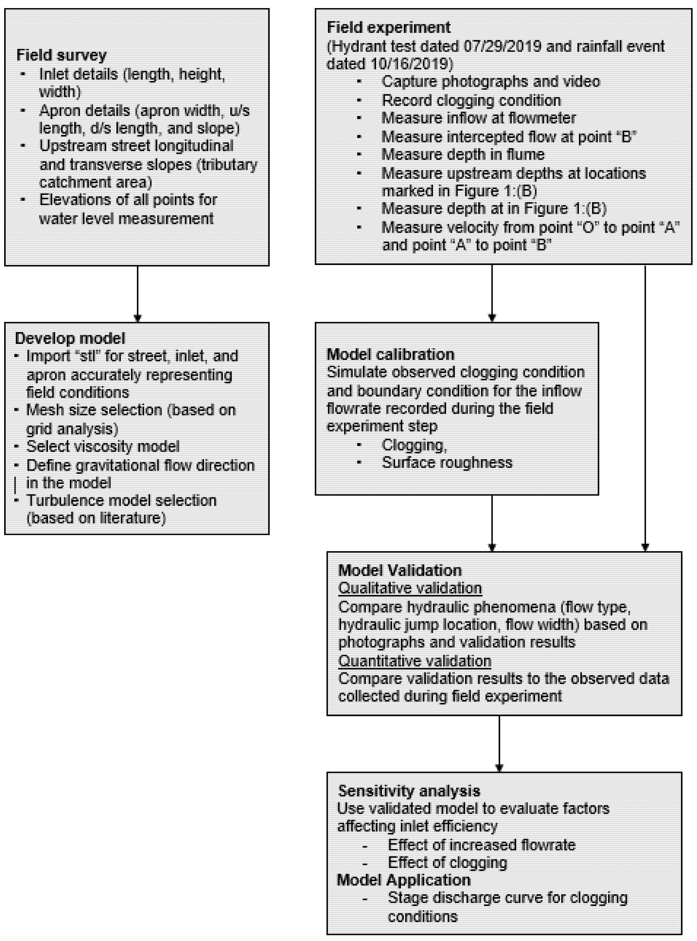
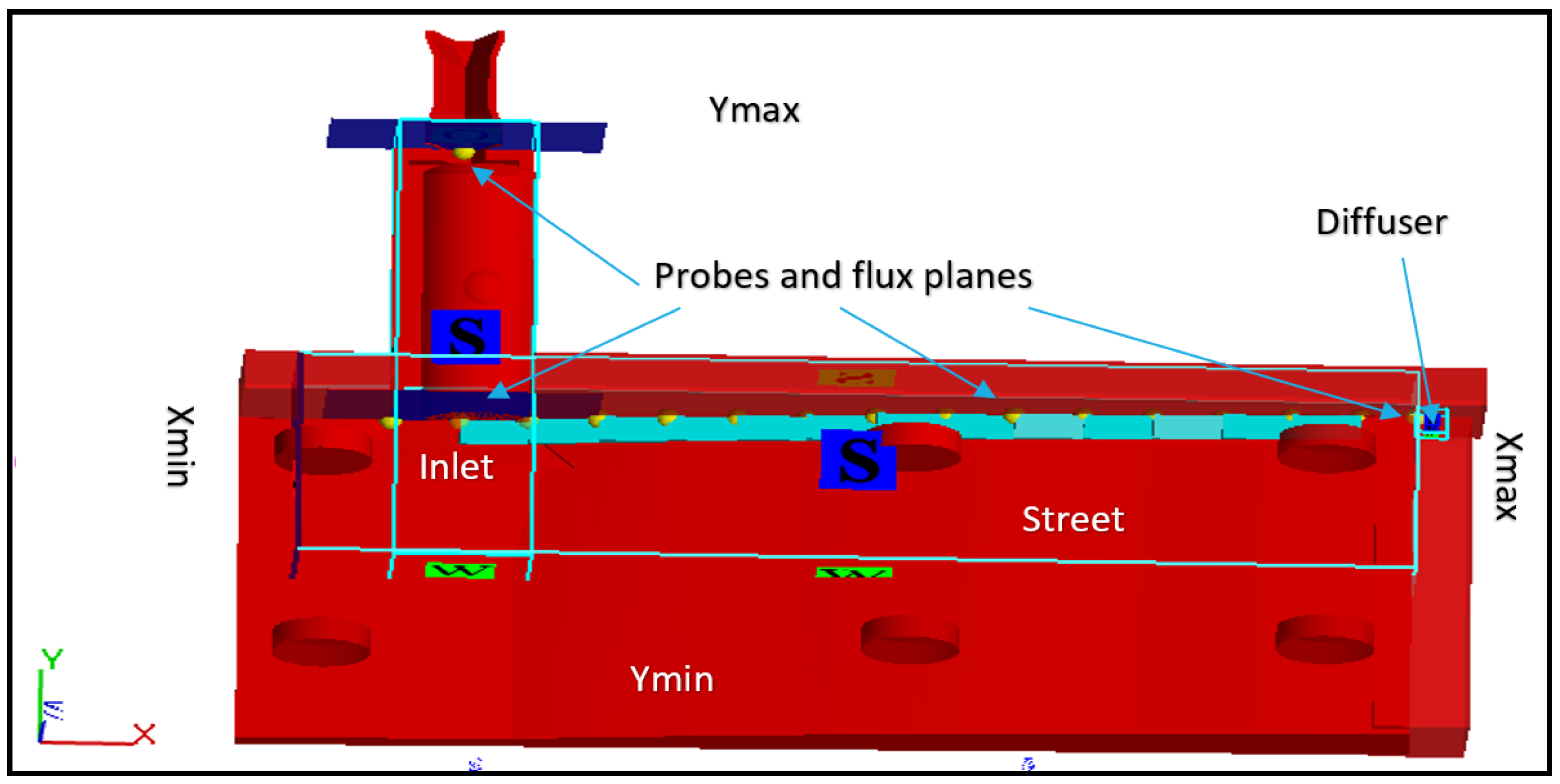
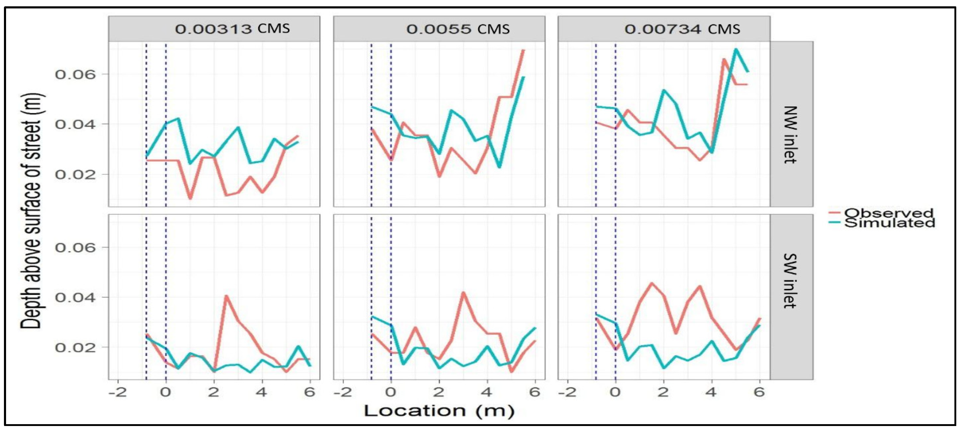
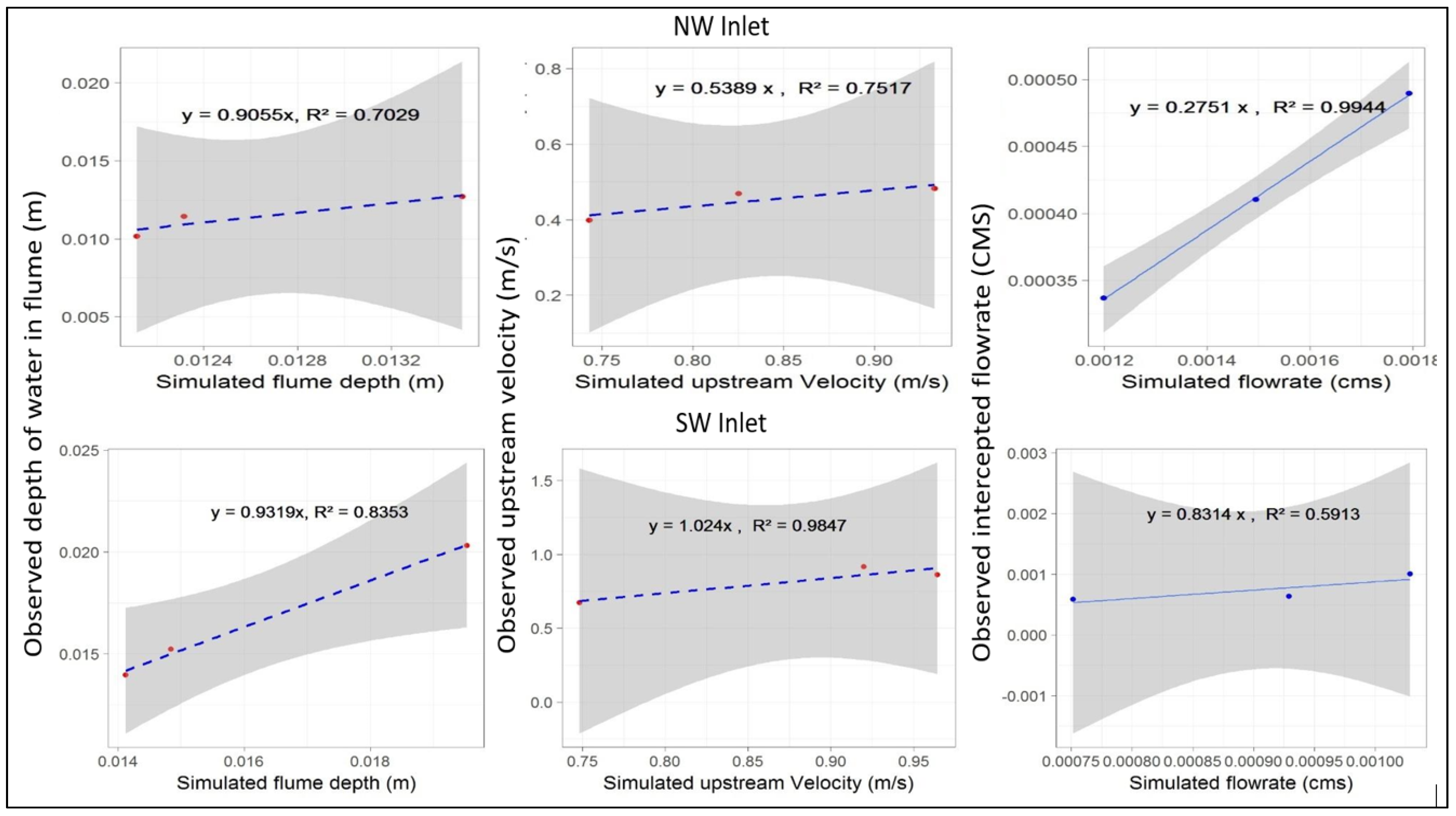
Taking advantage of the increasingly recognized value of CFD models as a cost-effective means of better understanding key flow processes, this paper develops, calibrates, and validates a CFD model to describe field conditions at an actual GI facility. The model domain was constructed using surveyed field data, and the model was calibrated and validated using five measurements made in the field: The (i) inflow rate, (ii) intercepted flow rate, (iii) upstream velocity, (iv) upstream flow depth, and (v) flow conditions immediately upstream and downstream the inlet. A sensitivity analysis of the validated model was used to investigate how inlet performance would vary under field conditions that differ from those found at this particular site.

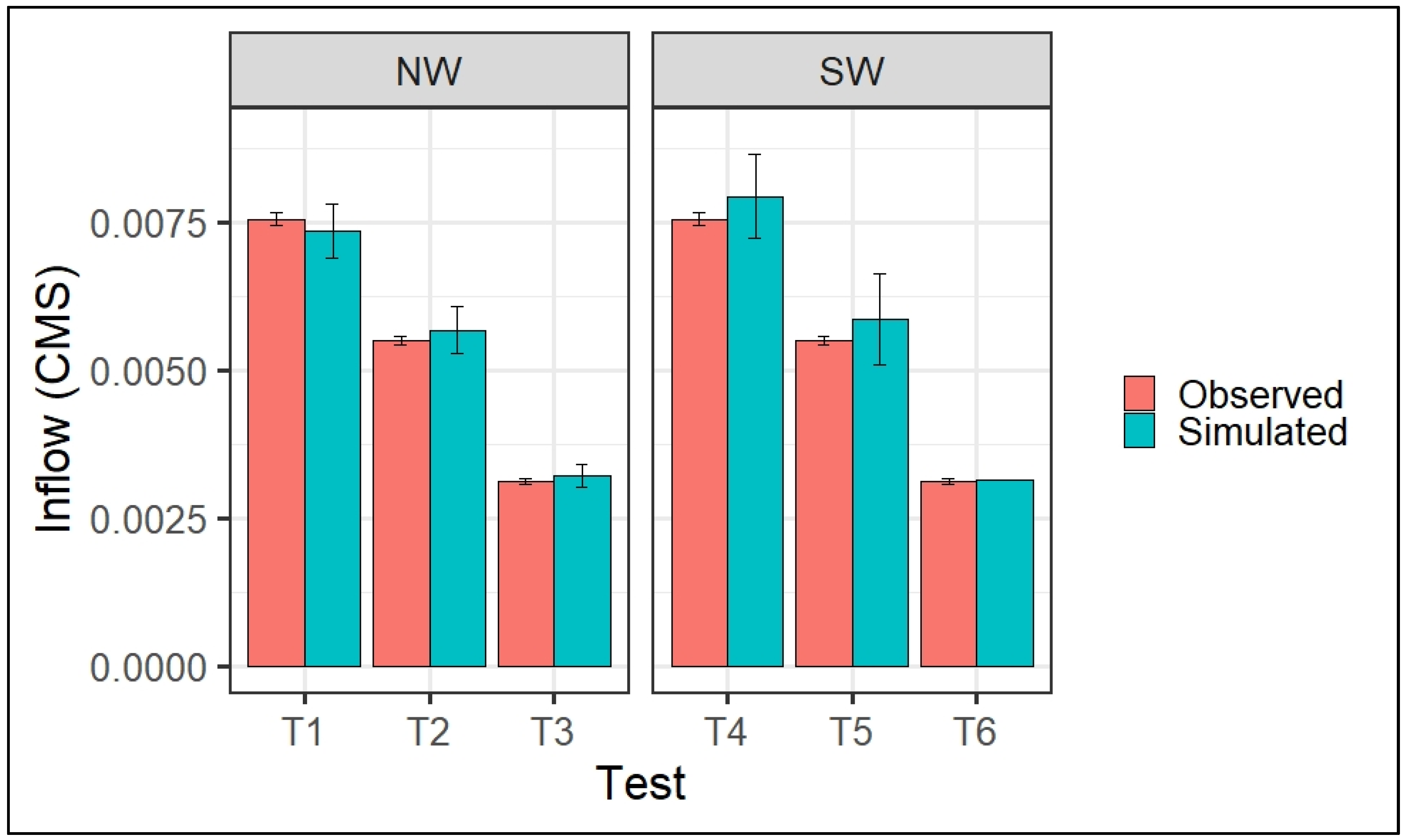
The paper is organized as follows. The procedure to gather observed data for these five parameters is described in Section 2.2. The model development is included in Section 2.3. Section 3 contains a comparison of the simulation results and observed data. Finally, the inlet hydraulics, effects of clogging, and increases in flow rate are discussed in Section 6.

2. Materials and Methods

2.1. Site Characteristics

The study site is a stormwater capture Greenstreet (SCGS) located on Crotona Parkway Malls, located on Southern Boulevard/Crotona Parkway between East 178th Street and East Tremont Avenue, Bronx, NY 10460. Instituted originally in the 1990s, the NYC Greenstreets program replaces unnecessarily paved surfaces within the public right-of-way with vegetated spaces [26]. Over the past decade, many greenstreets have been depressed below the street elevation and curb-cuts used to direct street runoff into them. This greenstreet was built in 2012 as a memorial for the 87 people killed in a local night club during an act of arson and is unofficially referred to as the “Happyland Greenstreet”.

The project added 256.8 m² (2764 ft²) of depressed vegetated beds into this area, with curb-cut inlets hydraulically connecting them to the surrounding street. The site’s total catchment area is 1242.2 m² (13,500 ft²), making its total hydraulic loading ratio of 4.8 to 1. The actual dimensions of the street, apron, and inlet geometries of each of the two inlets are presented in

Table 1. Street morphology and inlet geometry.

Physical Characteristics	Validation
Street width, curb to crown	3.5 m
Length of inlet	0.82 m
Opening depth of inlet	0.154 m
Upstream (U/S) gutter depression (apron) length	0.425 m
Downstream (D/S) apron length	0.425 m
Apron width	0.445 m
NW inlet upstream street slopes (Sx, SL)	1.50%, 1.18%
SW inlet upstream street slopes (Sx, SL)	1.15%, 1.30%

Note. Sx is the transverse slope of the street and SL is the longitudinal slope of the street.

. Although both inlets are on the same street, the longitudinal and transverse street slopes differ slightly between the two inlets. In addition, though the inlet length, inlet depth, apron width, and apron length are the same for both inlets, the tributary catchment area associated with the NW inlet is half of that of the SW inlet.

Figure 1A is a map of the site depicting its location in NYC. Figure 1B depicts three curb-cut inlets, labeled northwest (NW), southwest (SW), and southeast (SE), and showing the tributary areas to each of the three inlets. The dimensions of all three inlets, inlet channels, and apron section are presented in Figure 1C. After the flow enters through the curb-cuts, the intercepted flow passes under the sidewalk through rectangular channels pitched at 1% grade and covered with metal grates. Since the site was designed to be monitored, each rectangular channel discharges into a Tracom extra-large 60-degree V-notch trapezoidal flume, situated in cast-in-place concrete wingwalls (Figure 1D)—photograph of the SE and SW inlets. Figure 1B also contains a graphical representation of the physical conditions around the SW and NW inlets (not to scale) and the water in the experiment (detailed in Section 2.2.2) is dispersed at the “diffuser” marker (bottom right in Figure 1B) at a specific flow rate. Water that flows downstream along the curb can either flow into the inlet of the GI or bypass the inlet and continue down the curb.

The methodology is presented graphically in Figure 2, with individual steps described in the subsections that follow.

2.2. Fieldwork

2.2.1. Field Survey

The street morphology and inlet geometry, presented in Table 1 and Figure 2, were surveyed on the day of the hydrant test (29 July 2019). The elevations of all data points were measured using survey equipment with a 1.27 cm precision staff.

2.2.2. Field Experiments Using a Hydrant Test

A hydrant test was performed on 29 July 2019 to characterize the flow regime. The results of the hydrant test were verified during an actual rain event on 16 October 2019. The hydrant test procedure was as follows. First, a backflow preventer, flow gage (OMNITM meter), and diffuser (Pollard water—LPD-250) were connected to the hydrant, and the diffuser positioned 7 m upstream of the inlet as shown in Figure 1B. Flow measurements were recorded every minute with a 0.000472 cubic meter per second (CMS) precision. Next, for several key flowrates (described below), the hydrant was opened, and the flow regime allowed to stabilize over 15 min. Once the flow stabilized, the water depths in the upstream and downstream gutters, apron, and flume were recorded at 5-minute intervals; three measurements were taken at each observation interval, and the average depths at each location computed and logged. The locations of all flow depth measurement points are depicted with a red circle in Figure 1B.

The depth of water in the flume was used to compute the intercepted flow rate (Observed Qint) using a stage-discharge curve generated for the Tracom trapezoidal flume by recording the time required to fill a 3-L container for each flow rate. Each depth and flow rate pair were recorded three times to account for measurement error. Next, an equation was developed to describe the measurements, Equation (1).

$$Q_{int \left(on\text{-}site\right)}\left(\mathrm{CMS}\right) =0.7429 · H^{1.6776}$$

(1)

where Qint (on-site) is the intercepted flowrate (CMS) and H is the water level measured in meters in the flume at point “B” in Figure 1B.

At each experimental flow rate, the velocity upstream of the inlet was determined by dividing the distance between points “A” and “O” in Figure 1B by the observed time required for red dye injected into the flow regime at point “O” in Figure 1B to reach point “A”. The velocity in the flume was calculated using the same method, with the dye injected at point “A” and travel time measured to the outlet of the flume at point “B”.

2.2.3. Selection of Flow Rates for Field Experiment

Experimental flow rates were selected considering the accuracy of the flow meter, control of the hydrant valve, and the peak flow rate expected from the tributary area under specific storm conditions. Although the flow meter could theoretically measure flows as low as 0.000472 CMS, it was impossible to sustain steady flow rates in this range using the hydrant valve. For this reason, the minimum flow rate used in the test was 0.0023 CMS. By contrast, the highest flow rate was initially selected based on a Rational Formula evaluation of the peak rate of flow expected from a 10-year, 15-min storm, Equation (2):

$$Q =K·C·I·A$$

(2)

where,

• Q—inflow (CMS),
• K—conversion factor from English to metric units = 0.0028,
• C—dimensionless runoff coefficient = 0.9 for impervious street [5],
• I—precipitation intensity (mm/hr), and
• A—drainage area (0.0325 ha for the NW inlet and 0.065 ha for the SW inlet).

While the NYC Department of Environmental Protection (NYCDEP) requires that the 5-year storm with a 6-min time of concentration be used in the stormwater detention facility design [27], a 10-year return period is recommended by the Federal Highway Administration [5] for stormwater inlet design. The 15-min duration, 10-year storm was initially selected for field testing because its duration exceeds the time of concentration expected for an urban catchment such as this one [28]. The intensity associated with this storm was obtained by the intensity duration frequency (IDF) curves generated by NYCDEP [29] and verified against the National Oceanic and Atmospheric Administration’s Atlas 14 datasets [30].

However, flow at this rate triggered significant inlet bypass during a hydrant test. Consequently, field experiments at three other flow rates, corresponding to 15-min storms of 1, 2, and 5-year return periods were also performed. A complete list of all the flow rates tested at each inlet is shown in

Table 2. Flow rate selection—peak flow rate calculations based on peak rainfall intensity with a 15-min duration storm (NOAA, 2017).

Inlet	Flow Rate Tested at the Field (CMS)	Peak Flow Rate Calculated Based on the Rain Intensity Q (CMS)	The Nearest Equivalent to 15-min Duration Rain Intensity (mm/hr)	Corresponding Return Period (Years)
SW	0.0090	0.01032	63	1
NW	0.0055	0.00516	63	1
	0.0068	0.00614	75	2
	0.0075	0.00778	95	5
	0.0090	0.00909	111	10

. Since flow rates lower than those shown in Table 2 could not be simulated using the hydrant, an actual rain event occurring on 16 October, 2019 was used to verify the low-flow performance of the inlets. During this event, 100% of the runoff presented to both inlets was intercepted (despite significant clogging of the inlets with debris). The intercepted flow rate at the SW inlet was 0.00054 CMS and, further downgradient, the intercepted flow at the NW inlet was 0.00044 CMS. No manual measurement of the intercepted and bypass flows during any other actual storm was performed.

2.3. CFD Model Development

The CFD model was developed using FLOW-3D [31] (Flow Science Inc., Santa Fe, NM, USA) a multiphysics–CFD commercial code for general three-dimensional (3D) analysis.

2.3.1. Discretization and Surface Tracking Codes

The three-dimensional 3D Reynolds Averaged Navier–Stokes equation (RANS) was solved with a finite volume numerical scheme [32,33]. The open airflow is a mixture of water and air and the definition of this water-air boundary is difficult to assess as it changes over time as the water flow regime/pattern varies. Hence, the volume of fluid (VOF) methodology was used to define the free surface as a fixed mesh [33], eliminating the problem of mesh deformation. The algorithm tracks the shape and location of the free surface while maintaining its character as a discontinuity and applies proper free-surface boundary conditions to the mesh, shortening the simulation time [32,33]. The surface of calculation mesh was defined using VOF and the Fractional Area/Volume Obstacle Representation method (FAVOR^TM, Flow Science Inc., Santa Fe, NM, USA) [32,33]. The selection of specific mesh properties was also informed by the grid analysis, described in Section 2.3.4.

2.3.2. Turbulence Model Selection

RANS requires simulation of turbulence, and FLOW-3D supports six different turbulence models: The Prandtl mixing length model, the one-equation, the two-equation K-epsilon (k − ε), renormalization group (RNG), k—omega (k − ω) model, and a large eddy simulation (LES) model. Gomez et al. [18] conducted a sensitivity analysis on three turbulent models (LES, RNG, and the k − ε), and determined negligible differences (e.g., ±1%) for intercepted flow rates of up to 0.01 CMS. Of these, RNG has the advantages of requiring fewer oscillations and incurring a lower computational cost [18], and previous researchers have used it in open channel flow applications with the VOF method [34]. RNG turbulence was selected for this application, with the maximum turbulent mixing length set to compute dynamically, and the gravitational force in the Z-direction Z set to −9.81 m²/s.

2.3.3. Time Step and Initial Condition

A transient simulation was performed to track the water-air interface continuously. The time step of the transient simulation was computed dynamically by the FLOW-3D code. All terms of RANS are computed from current time-step values with an explicit numerical scheme for each variable. The explicit approach generates an optimized efficient numerical scheme with limited time-step values that ensure the stability and accuracy of results. The initial condition was set to hydrostatic pressure, and did not interfere with the solution because it was only used for early convergence.

2.3.4. Mesh Size Selection and Definition of Boundary Conditions

A three-dimensional drawing was imported to FLOW-3D in a “stl” format to characterize the physical characteristics of the inlet tributary area and inlet. The geometry was divided into structured hexahedral 3D grids. The model consisted of three meshes, street, inlet, and diffuser. The inlet length was 0.82 m, and flow depth measurements were made at 0.5 m sections upstream of the inlet. This model is shown in Figure 3.

2.4. Grid Analysis

The finest grid with 1 M cells (for 0.00313 CMS) had an error of ±0.5% but the computational time was longer than 36 h. With 397k cells, for 0.0055 CMS flowrate the simulation took longer than 11 hours to complete but yielded the lowest absolute error in prediction of inlet efficiency (±0.03%). The model consisting of 227k and 198k cells had an absolute error of 3.5% and 3.9%, respectively but the 227k model took longer than eight hours whereas the 198k model took a little longer than one hour. As the number of cells decreased further from 162k to 93k the absolute error in predicting the inlet efficiency was reduced by 9%, with the computation time decreased from 41 to 17 minutes, respectively. Hence, to reduce the computation cost keeping absolute error in predicting inlet efficiency less than 5%, the grid with a total number of cells of 198,032 was selected for the final model as one of the goals of this paper is cost-effectiveness.

Table A1. Error analysis for 0.0055 CMS.

# Cells	Modeled Inflow (CMS)	Observed Inflow (CMS)	Relative Error (%)	Modeled Inlet Efficiency (%)	Observed Inlet Efficiency (%)	Absolute Error (%)
596311	0.00535	0.00552	-3.07971	14.39000	11.95000	2.44000
397833	0.00553	0.00553	0.05134	11.98535	11.95000	0.03535
227896	0.00558	0.00552	1.08696	15.45000	11.95000	3.50000
198032	0.00586	0.00552	6.15942	15.87000	11.95000	3.92000
194635	0.00590	0.00552	6.88406	16.00000	11.95000	4.05000
162023	0.00600	0.00552	8.69565	18.28000	11.95000	6.33000
93754	0.00660	0.00552	19.56522	26.23000	11.95000	14.28000

included in the Appendix A that presents an error analysis for the 0.0055 CMS inflow rate and inlet efficiency.

2.5. Definition of Boundary Conditions

The model simulation mimicked the field experiment, with the flow introduced to the system seven meters upstream of the inlet. The water attained a steady state depth of 0.5 m from the diffuser location on its way toward the inlet. The diffuser was set up as a separate mesh transferring water into the street mesh in the model. The Xmax (Figure 3) boundary condition for the diffuser was set to a constant volume flow rate during the simulation with specific flow rates selected for both validation and parametric analysis purposes. The size of the diffuser mesh matched the actual diffuser dimensions. The Ymin boundary was set to “wall” to avoid the loss of water through the boundary to replicate the experiment. The Zmin condition was set to “wall” as the street is impervious. The Ymax boundary condition for the street was selected as “symmetry” and for the inlet as “outflow.” The Xmax condition for both the inlet and the street was set as “symmetry,” and Xmin was set as “outflow.” The viscous flow and no-slip wall shear conditions were used for all the “wall” boundaries. Onsite observations indicated that the cars frequently park in front of the inlet, as was the case during the hydrant test. To represent this condition, a standard car tire was added to the model domain (also shown in Figure 3) based on conditions observed during the hydrant test.

2.6. Replicating Inlet Clogging

Site observations made previously by the authors between 2015–2017 (as part of a separate study) indicated that inlet clogging was a frequent phenomenon at this site. Indeed, during the 2019 hydrant test, the inlet was found to be clogged (Figure 4A). To represent these conditions in the simulations, obstructions blocking the opening in the simulated inlet were added to the model domain, as illustrated in Figure 4B. As the debris did not move with the water flow and water was flowing constantly around the debris during the test, a solid blockage was used in the model to represent this. The model was calibrated by adjusting the percent clogging from 75% to 90% and comparing the inlet efficiency to the observations. The percent clogging that best matched the inlet efficiency was selected for sensitivity analysis. Blockage of 85% and 88% of the inlet best represented the inlet efficiency, for the SW and NW inlets, respectively.

2.7. Surface Roughness

Manning’s n for overland sheet flow can vary between 0.013–0.016 for asphaltic road surfaces [5]. At this site, the tributary area to the inlet was characterized by potholes and irregular surfaces. Such irregularities have been found responsible for non-negligible differences in flow patterns at low flows (~25 L/s), causing a relative model error of 23% in [18]. Other researchers [35] have, however, indicated that these discrepancies were localized and limited in RNG simulations.

In FLOW-3D, surface roughness is represented by a depth, k. Four different roughness conditions (k = 0.001, 0.005, 0.0076, and 0.01) were considered in the model calibration process. For each roughness value, the simulated and observed inlet efficiency was compared. The surface roughness corresponding to the best-matched inlet efficiency was selected. All the values of k produced an inlet efficiency and flow rate within 10% of one another, but with k = 0.0076 m (equivalent to a manning’s n of 0.018 [18,36], the intercepted flow rate was within ±40% and depth was within ±10% compared to the observations for the SW inlet and the same was used for the NW inlet).

2.8. Inlet Performance Metric

The efficiency of the inlet during both the observed and simulated conditions was evaluated using Equation (3) the inlet efficiency (E) [5], defined as the ratio of intercepted flow by the inlet Qint (CMS) to the approaching inflow Q (CMS) at steady state:

$$E (\%)=\frac{Q_{int} }{Q }·100$$

(3)

The inlet efficiency (E) can vary between 0% and 100%, with 0% indicating no flow into the inlet, and 100% representing interception of all presented flow. The mean relative error, defined as the ratio of absolute difference between the observed (depth, velocity, or flow rate) and modeled quantity to the observed quantity (depth (m), velocity (m²), or flow rate (CMS)), was also computed per Equation (4)).

$$MRE (\%)= \frac{1}{N} {{\displaystyle \sum }}_{i=1}^N\left|\frac{\left(Quantit{y}_{modeled}-Quantit{y}_{observed}\right)}{Q_{uantityobserved}}\right|·100,$$

(4)

2.9. Convergence Assessment

Due to the nature of transient RANS simulation used by FLOW-3D, the determination of solution convergence is complicated. FLOW-3D dynamically assigns a very small-time step value along with very few iterations per time step via a self-corrective procedure as well as an automatic setting of the convergence criteria. Variations of this changing convergence criteria can be observed using the pressure residual values which averaged around 5e-05, lower than the typical maximum of residual of 1e-03 [37]. However, it is more important to assess convergence for the entire simulation instead of an individual time step. While this simulation is transient, it can be treated as a steady problem with fluctuation over a larger time scale. By examining mass flow rate fluctuation over time, we observed stabilization of flow rate after 5 s of simulated time. This stabilization is an indication that the overall flow has reached convergence. A further discussion of this flow rate can be found in the validation results below.

3. Validation Results

The CFD model results were compared with the experimental results qualitatively and quantitatively. The CFD model was primarily calibrated and validated to replicate the observed inlet efficiency. These calibration and validation results are presented in this section. Additionally, five parameters were validated by comparing model results to the observations: (i) Inflow flow rate, (ii) intercepted flow rate, (iii) upstream velocity, (iv) upstream flow depth, and (v) flow condition before and after the inlet (these results are included in the Appendix A).

3.1. Qualitative Validation

The flow regimes observed during the hydrant tests at each flow rate were photographed and video recorded for later comparison with three-dimensional simulations produced using the CFD model. One of these scenarios is depicted in Figure 5. The flow pattern predicted by the CFD model matched the field observations well. For example, the model accurately simulated how the flow split and spread around the car tire. The lighter the blue, the higher the flow depth in Figure 5 (right screenshot of the model). The depth of flow upstream of the inlet was lower than the depth of flow in front of the inlet, with a hydraulic jump observed. These observations suggest that the model accurately represents key aspects of inlet hydraulics that are related to inlet efficiency.

3.2. Quantitative Validation

Comparison of observed and simulated inflow rates (e.g. flow presented to the inlet), intercepted flow rates (e.g. flow into the inlet), flow profiles, depths, and velocities were used for a quantitative validation of the model.

Figure 6 is a comparison of the observed and simulated inflow rates during the hydrant test. The error bars on the “observed” columns represent the standard error in the field observations. The error bars on the “simulated” columns represent the standard deviation of the inflow rates over the transient simulation. For all tests at both inlets, the observed and simulated flows show reasonable agreement. Both models were found to accurately represent the lower flow rates associated with no bypass.

Table 3. Comparison of simulation results to observations.

Inlet	Test	Simulated Inflow (CMS)	Observed Inflow (CMS)	Relative Error—Inflow Flowrate (%)	Simulated Intercepted Flow (CMS)	Observed Intercepted Flow (CMS)	Relative Error—Intercepted Flowrate (%)	Modeled Inlet Efficiency (%)	Observed Inlet Efficiency (%)
NW	T1	0.00735	0.00736	−0.13	0.00179	0.00049	−265.30	24.35	6.65
NW	T2	0.00567	0.00566	0.17	0.00150	0.00041	−265.85	26.45	7.24
NW	T3	0.00322	0.00330	−2.42	0.00120	0.00034	−252.94	37.26	10.30
SW	T4	0.00794	0.00755	−5.16	0.00103	0.00108	−4.62	12.97	14.30
SW	T5	0.00586	0.00552	−6.15	0.00093	0.00066	40.90	15.87	11.95
SW	T6	0.00315	0.00314	−0.31	0.00075	0.00057	31.57	23.80	18.15
NW	T1	0.01212	0.01016	−19.24	0.93313	0.48263	−93.34	0.48263	−93.34
NW	T2	0.01232	0.01143	−7.75	0.82539	0.46904	−75.97	0.46904	−75.97
NW	T3	0.01350	0.01270	−6.31	0.74312	0.39904	−86.22	0.39904	−86.22
SW	T4	0.01953	0.02032	3.88	0.91998	0.91575	−0.46	0.91575	−0.46
SW	T5	0.01484	0.01524	2.62	0.96437	0.86207	−11.86	0.86207	−11.86
SW	T6	0.01412	0.01397	−1.07	0.74851	0.67295	−11.22	0.67295	−11.22

presents a comparison of simulated and observed inlet efficiency. The absolute error between modeled and observed inlet efficiency for the NW inlet was ±20% and for the SW inlet was ±4%.

The simulated and observed velocities and depths are also presented in

Table 4. Flow rate selection criteria.

Flow Rate (CMS)	Selection Reference
0.00044	Observed inlet capacity during precipitation event dated July 29,2019
0.001	Interpolation
0.0028	Interpolation
0.0033	Hydrant test
0.0055	Hydrant test and intensity corresponding to 15 min duration, 1-year return period with NW inlet
0.0068	Interpolation
0.00755	Hydrant test and intensity corresponding to 15 min duration, 5-year return period with the NW inlet, and less than 1-year return period for the SW inlet

. The models replicated the observed upstream average flow depths to within ±30% and ±10% for the NW and SW inlets, respectively. The NW model predicted the flow depth in the flume to within ±20% of the observed. The SW model replicated the observed flow depth in the flume by ±4%.

Table 3 also compares the simulated and observed upstream velocities. Though both models over-predicted the upstream velocities, the simulated and observed upstream velocities were linearly correlated, as discussed in Appendix A.2. The mean relative error in velocity predictions for the SW inlet was less than ±6%. All the simulations resulted in a supercritical flow upstream of the inlet, with flow depth increasing downstream of the inlet, as the flow became subcritical. As expected, a hydraulic jump was observed near the inlet itself (Figure 5A) and was replicated in the simulation. The lighter blue shade in front of the inlet (Figure 5B) represents a lower depth, thus a supercritical condition. The simulated and observed flow profile over the street surface are presented in the Appendix A—Figure A1.

4. Scenarios for Sensitivity Analysis

The sensitivity analysis focuses on the extent to which inlet clogging, determined by the effectiveness of GI maintenance practices, and runoff flow rate, which is greater at higher intensity storms and higher tributary areas, are related to inlet performance.

4.1. Effect of Flow Rate on Inlet Efficiency

Table 4 lists seven different flow rates used in the sensitivity analysis. These values include flow conditions in which the inlet was observed to be 100% efficient (0.00044 CMS) as well as higher flow rates during which bypass of the inlet was observed during the field experiment.

4.2. Effect of Clogging on Inlet Efficiency

The sensitivity analysis considers six clogging conditions varying from 0–90%, also reflecting observed conditions. A survey conducted on 11 USA cities by the San Francisco Budget and Legislative Analyst’s Policy Analysis Report [38] reports street cleaning frequencies ranging from 0–5 times/week. In NYC, streets are theoretically swept twice a week, and in addition, the NYC Department of Environmental Protection regularly maintains GI systems, cleaning their inlets. However, field observations by the research team suggest that some streets are never swept, and many inlets are partially or fully obstructed by debris and trash (see Figure 5). Though it is well known that clogging reduces inlet efficiency [39], no research on clogging of this particular inlet geometry has been published.

Considering six different inlet clogging conditions and seven different flow rates, the sensitivity analysis featured a total of 42 simulations for each inlet, as presented in

Table 5. Model scenario matrix depicting the number of model runs at each flow and clogging condition.

Clogging Conditions	Flow Rate (CMS)							Total for NW Inlet	Total for SW Inlet
	0.00044	0.001	0.0028	0.0031	0.0055	0.0068	0.00755
0%	1	1	1	1	1	1	1	7	7
10%	1	1	1	1	1	1	1	7	7
25%	1	1	1	1	1	1	1	7	7
50%	1	1	1	1	1	1	1	7	7
75%	1	1	1	1	1	1	1	7	7
90%	1	1	1	1	1	1	1	7	7
Total	6	6	6	6	6	6	6	42	42

. The efficiency of the inlet at each of these simulations was computed, and contour plots generated to display the results. Because the roughness of the tributary areas of the two inlets varied, a comparison of the contour plots generated for the two sites gives some insight into the role of this parameter in the results.

5. Sensitivity Analysis Results

The sensitivity analysis results for the NW and SW inlets are presented in Figure 7 and Figure 8, respectively. The effects of flow rate and inlet clogging on inlet efficiency are described, respectively, in the subsections below.

5.1. Effect of Flow Rate on Inlet Efficiency

In general, as flow rates increase, the efficiencies of both inlets decreased. However, the reduction in efficiency differed by inlet. At the lowest level of clogging, the efficiency of the NW inlet decreased from 100%, at the lowest simulated flow rates, to 25–30% at the highest flow rates tested. For the SW inlet, a flow rate of up to 0.0005 CMS was intercepted completely, with further increases in flow decreasing to no lower than 60%.

5.2. Effect of Inlet Clogging on Inlet Efficiency

Except for the lowest flow rates, the efficiencies of the inlets decrease as clogging increases. However, the flow rate above which clogging matters differs by inlet. For the NW inlet, clogging has a pronounced effect on inlet efficiency at flows exceeding 0.003 CMS. By contrast, the efficiency of the SW inlet is compromised by clogging at flows exceeding 0.001 CMS. At the highest level of clogging and highest flow rates, both inlets depicted efficiencies of lower than 15%.

Sedimentation significantly reduced the efficiency of the NW inlet, and increased model error. The NW model overestimated the intercepted flow rate by 200%, and the velocity by 93%, and was thus not used directly in the sensitivity analysis. However, although the NW model could not accurately replicate the intercepted flowrates due to the deposition of sediment into the inlet, it was still precise. The simulation of intercepted flow rates was linearly correlated to the observed. This correlation equation (described in Figure A2 of Appendix A) was used to predict intercepted flow rates, that were used to estimate the inlet efficiency. The efficiency of the NW inlet dropped significantly as clogging increased above 25%, e.g., to 10–20% efficiency. As the flow rate increased, the inlet efficiency dropped significantly for higher clogging conditions from 30% to 10% for the NW inlet. These observations underscore the importance of keeping inlets sediment free.

6. Discussion

The SW inlet model was, qualitatively and quantitatively, a better fit to the observations than the NW model, and possible explanations for this discrepancy are discussed below.

6.1. Possible Sources of Error in Model Validation

6.1.1. Velocity Measurements

It is challenging to record velocity in the field. The observed velocity is calculated upstream of the inlet. It is essentially the time of fluid travel from one point to another. The model was validated for three to five data points. The velocity was measured over a section of 5 m in the x-direction. The RNG turbulent model used in this study also calculated the average depth over velocity but at smaller intersections. Though the model is correctly representing the inlet hydraulics qualitatively, these issues most likely resulted in the high relative errors in velocity measurements.

6.1.2. Survey Data

Due to budget constraints, the research team did not have access to high precision (3 mm resolution) terrestrial (ground-based) LiDAR data to conduct the survey. Instead, the site was surveyed using the total survey equipment with a 1.27 cm precision staff. During the survey, cars were parked on the street, partially obstructing the view of the laser level, and traffic was heavy, limiting the amount of time the survey crew could spend in the street. It is possible these observational and logistical constraints could have introduced errors into the surveyed data.

6.1.3. Differences in Street Slope and Apron Slope

Due to street resurfacing conducted after construction of the greenstreet, the apron slopes and longitudinal street slopes upstream of the two inlets differed significantly. Two related factors may explain the better fit of the SW inlet model to its observations, as compared to the NW inlet. The slope of the street upstream of SW inlet was 2.38%, an increase when compared to the slope shown on the GI design drawings. In addition, while the designed slope of the apron was 10%, the actual slope of the 1-m section of apron extending upstream of the inlet was approximately 20%. These slopes were captured by the model. The NW model could not accurately capture the deposition of silt in front of the NW inlet. These factors would have made the SW inlet’s efficiency closer to normative conditions assumed in the CFD. (A more detailed exploration of the effect of apron design on inlet efficiency is evaluated in a companion paper focusing on the SW inlet).

6.2. Effect of Inlet Hydraulics on Inlet Efficiency

The NW and the SW inlets are on the same side of the street, yet their observed performance was significantly different. Although the CFD model predicted the hydraulic characteristics of the flow regime (e.g., flow rates, velocities, and depths) of the NW inlet less accurately than the SW inlet, the NW inlet’s observed efficiency was represented reasonably well. This section focuses on the effect of inlet hydraulics on inlet efficiency.

6.2.1. Inlet Hydraulics—Effect of Upstream Velocity and Its Effect on Formation of Inlet Clogging

Figure 9 portrays the simulated longitudinal (in the x-direction) depth-averaged velocity. In the supercritical flow regime, the maximum longitudinal velocity occurs near the downstream end of the inlet and near the free surface. Immediately after that point, the velocity drops and reaches its lowest value. This hydraulic behavior predicted by the CFD simulation is consistent with the literature [37]. Therefore, the CFD simulation provides additional hydraulic data that is difficult to collect in the field. The velocity reduces as the water spreads into the inlet channel, and, as the momentum is lost, the sediments start to deposit into the channel. The simulation results for a no clogging condition Figure 9 (left) indicated that the left side of the channel had a higher velocity than the right side of the channel. Greater sediment deposition was observed in the right side of the channel compared to the left side of the channel. The average velocity upstream of the SW inlet was 0.9 m/s, a non-silting, non-scouring velocity. The sediments are carried along with the flow and will be deposited downstream and into the GI system. The non-silting velocity is the minimum permissible velocity considered in a sewer or canal design. This is the minimum velocity required to avoid sedimentation and the growth of vegetation induced due to sedimentation. Sedimentation and growth of vegetation decreases the carrying capacity and increase maintenance costs [40]. The streets are swept once or twice a week. Storms between street cleanings will transport the sediments from the street with the flow. An average velocity of 0.6–0.9 m/s is required to prevent sedimentation in the inlet [41,42]. If the velocity is higher than 0.9 m/s, the sediment will most likely be deposited into the GI or transported downstream of the inlet with bypass flow.

The site observations also support the model results (photograph included in Appendix A—Figure A3). As the flow approaches the curb-cut inlet, runoff from the street entering the GI system hydraulically resembles flow in an open channel with a side weir. Discharge through the side weir depends on the upstream velocity and depth of water. One explanation for differences in the performance of NW and SW inlets could be the upstream velocity. Upstream of the SW inlet, the average velocity was 0.9 m/s, whereas the flow upstream of the NW inlet averaged 0.5 m/s.

6.2.2. Effect of Upstream and Downstream Flow Condition on Inlet Efficiency

The variation of the surface profile occurs due to the reduced discharge in the downstream direction along the length of the inlet, as a portion of street flow enters through the inlet. The upstream water depth is less than the critical water depth, resulting in a hydraulic jump. The location of the hydraulic jump varies with the upstream flow depth and velocity. Supercritical flow conditions before the inlet are due to the accelerated flow through the inlet opening. The graphical presentation along with the explanation is included in (Figure A4) in the Appendix A.

6.3. Model Application—Effect of Inlet Clogging on the Stage-Discharge Curve of Flume Fitted into the Inlet

As mentioned in the Methods, the stage-discharge curve provided by the manufacturer for the trapezoidal flume was used to convert the observed depth of flow to an intercepted discharge. However, the field investigation revealed that the inlets were typically clogged, and the sensitivity analysis illustrated how clogging can change the inlet efficiency. These observations implied that inlet clogging invalidates the stage-discharge curve provided by the manufacturer because the actual cross-section of flow is less than the theoretical.

The CFD model was used to assess the effect of clogging on the stage-discharge curve. Figure 10 illustrates the change in the relationship of the simulated flow depths and simulated discharge flow rates for four clogging conditions. The head-discharge curve changes drastically as the clogging increases above 50%. The data were fitted with a power law model. The coefficient of determination R² decreases from 0.96 to 0.7 as clogging increases from 0% to 75%. It further drops down to 0.5 as the clogging increases to 85%.

7. Conclusions

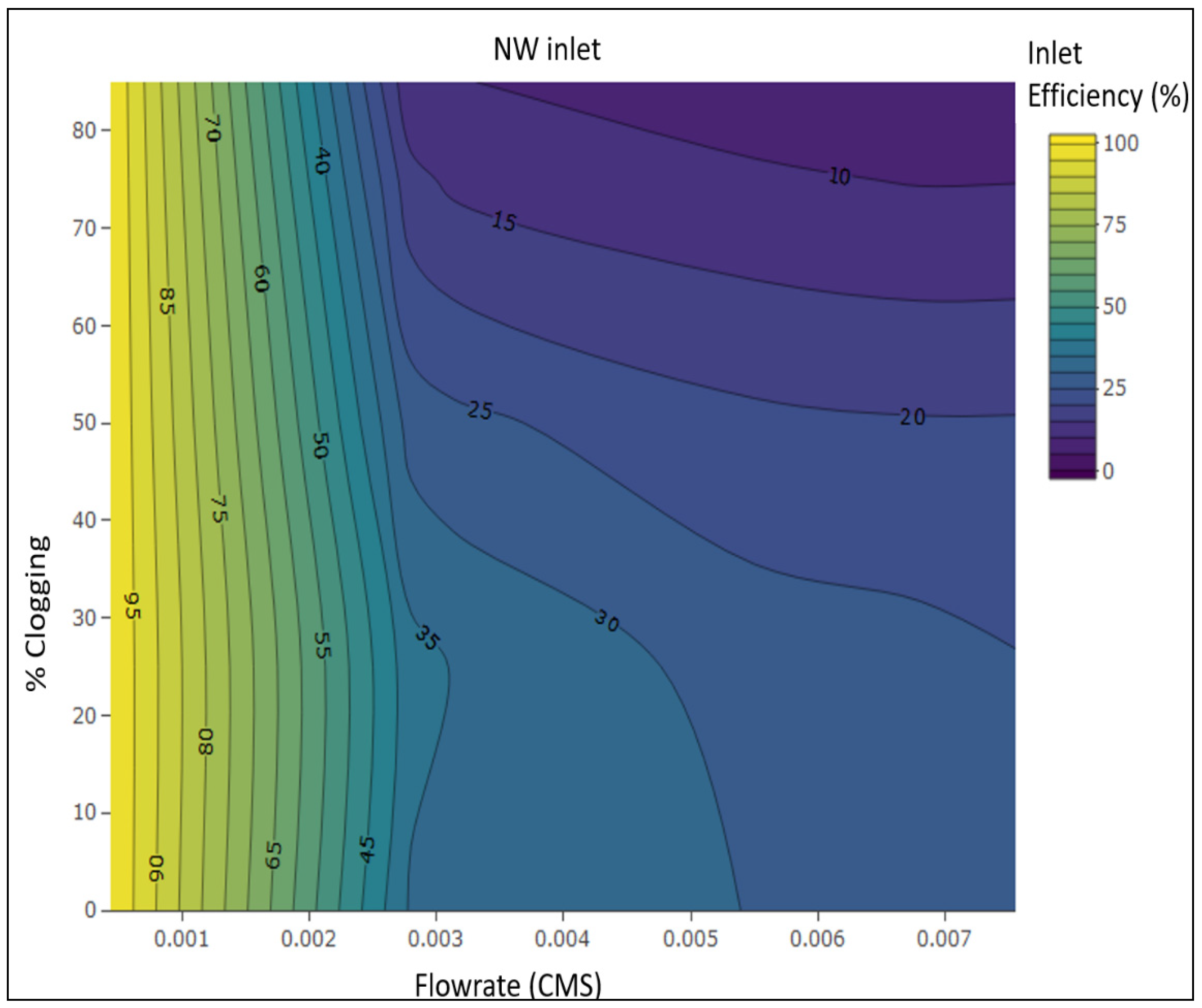
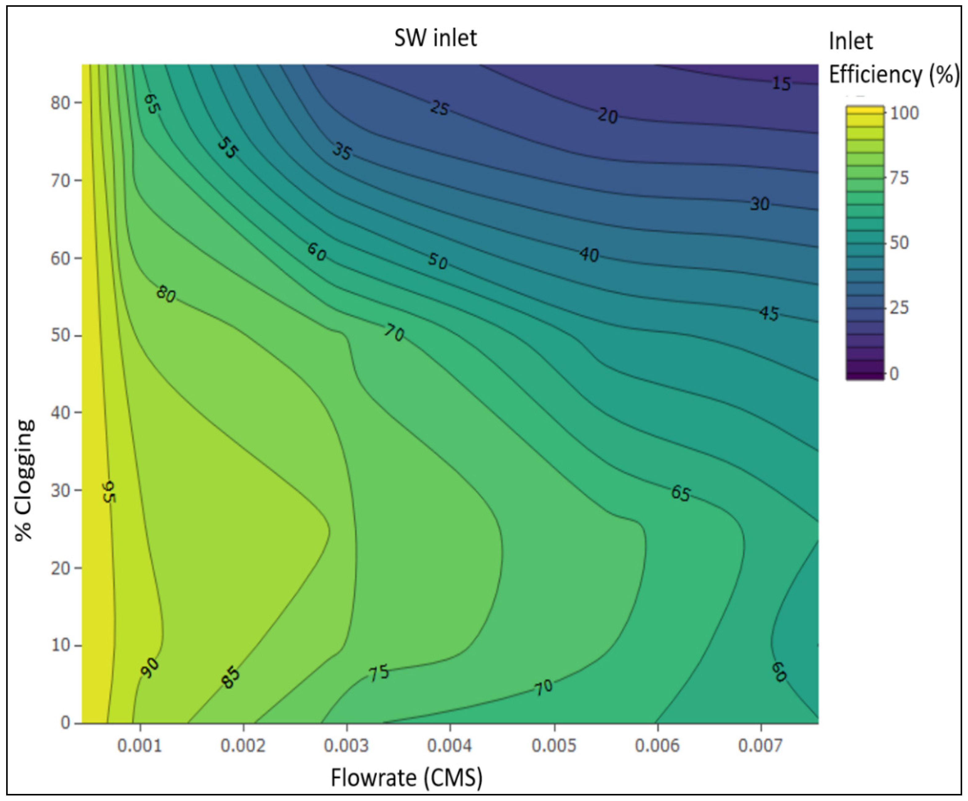
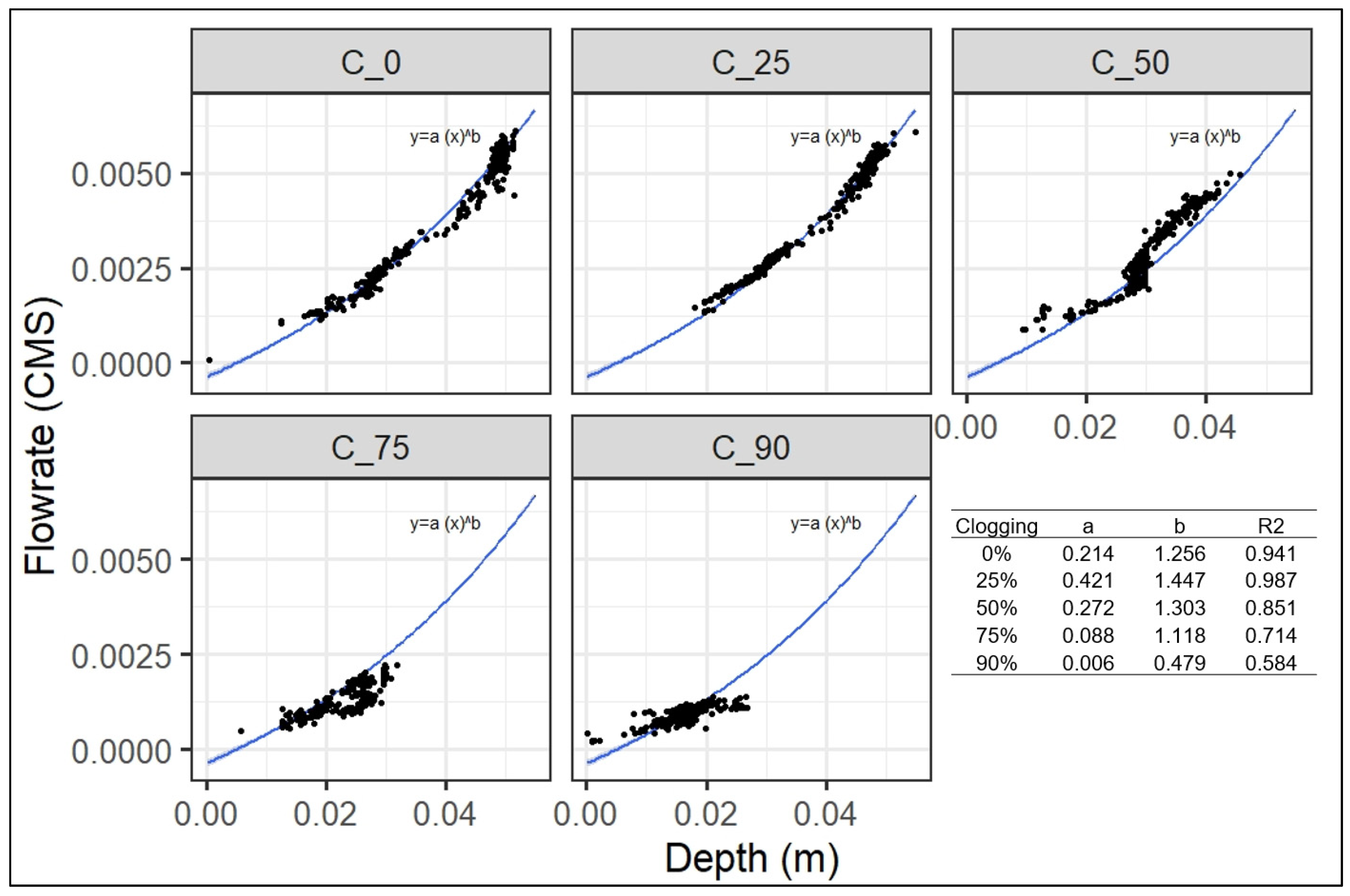
The study confirms that hydraulics play an important role in GI performance. This study underscores the importance of inlet clogging and other morphological differences in determining inlet efficiency at a range of flow rates. The research determined that inlet efficiency is likely to be lower at higher flow rates, as would be expected at higher tributary areas and increasing precipitation intensity. The research also reveals that inlet efficiency is reduced due to inlet clogging, emphasizing the importance of adequate maintenance of inlets in urban environments.

The field study underscores the importance of quality control during and after GI construction, and of careful monitoring of street resurfacing. At this site, field conditions differed significantly than those prescribed on the design, suggesting that performance predictions made based on the design drawings would deviate significantly from actual.

The CFD models were able to reasonably replicate inlet hydraulics and inlet efficiency. For sites with complex tributary area characteristics, CFD models thus offer a viable alternative to laboratory studies.

In conjunction with the CFD models, the hydrant tests were an effective approach to inlet monitoring that did not require installation of expensive on-site instrumentation. The hydrant test provided a controlled environment in the field that helped to calibrate and validate the model.

The research suggests that under real world conditions, stage discharge curves provided by flume manufacturers, developed in controlled laboratory environments, could deviate significantly from observed. In situ verification is recommended.

Design Implications

To increase the ability of GI systems to adapt to climate change, inlet length and apron should be designed to intercept 100% of the presented inflow during flow rates specified by local policy.

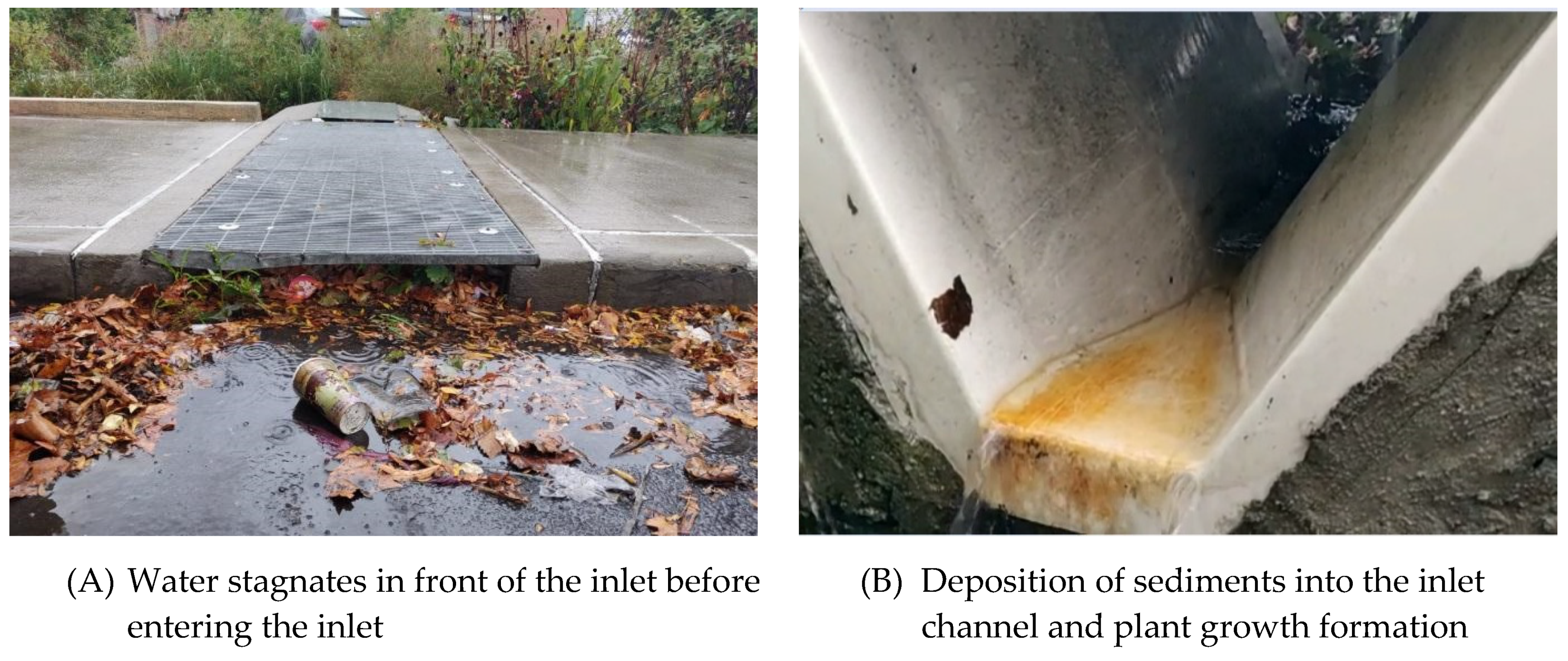
A comparison of the model validation attempts at the two inlets suggests that milder longitudinal street slopes (e.g., <1.5%) can cause silting upstream of the inlet. GI on mild street slopes should be designed with an inlet that minimizes silt deposition. If curb-cut inlets are used in such locations, they should have both additional apron depth in front of the inlet and into the GI to maintain a free outfall condition.

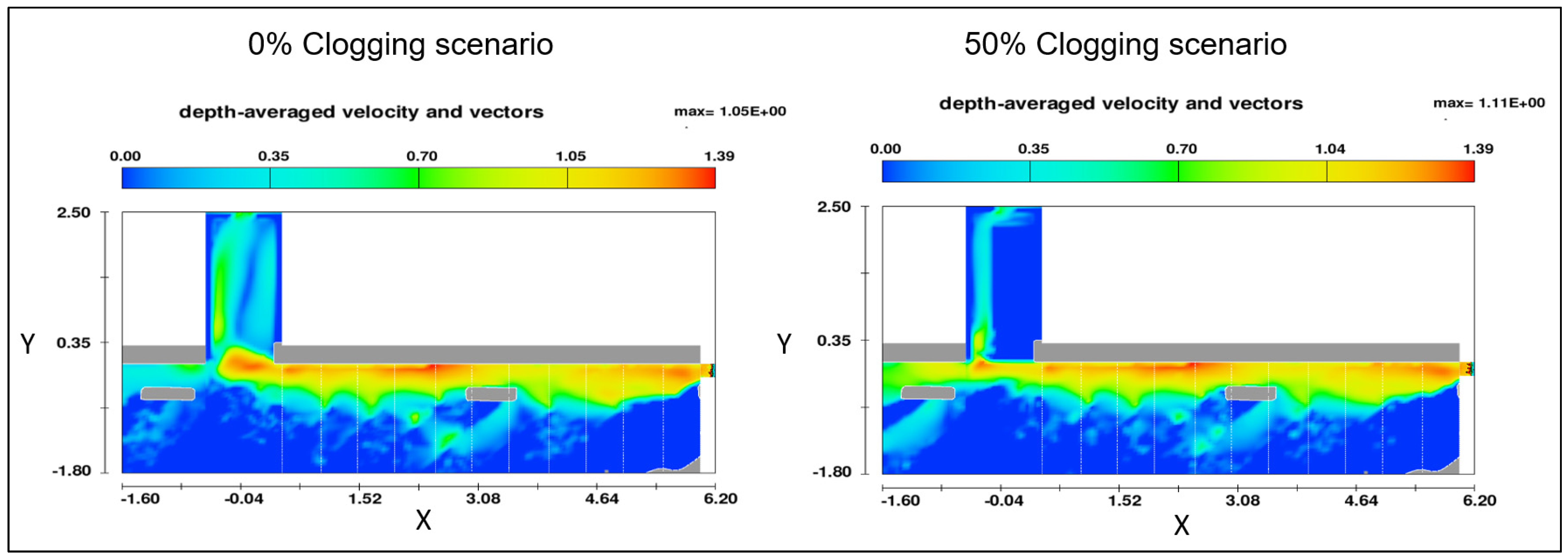
Inlet performance is reduced significantly with higher clogging under intense flow rates. Sediment deposition in the inlet channel and in front of the inlet (apron section) and clogging of the inlet with ordinary trash can both reduce inlet performance, especially under high intense rainfall conditions. The inlet and upstream tributary catchment areas should be cleaned frequently during the fall to remove leaves to improve the inlet performance.

Studies on other inlet design parameters such as apron design, inlet length under various street morphological conditions (transverse and longitudinal slope), and range of flow rate should be conducted to formulate design specifications for GI inlets to increase their hydraulic performance.

Differences in inlet performance suggest that efforts to upscale GI performance linearly could introduce significant errors into watershed estimates of stormwater capture.

GI design must consider local morphological conditions such as street slopes, inlet lengths, and inlet geometry. While upscaling the model results, inlet efficiency should be included. Sewers and canals are designed to have non-silting and non-scouring velocities. Such minimum and maximum velocity at the planned GI locations should be determined. The minimum velocity upstream of the GI inlet should be in the range of 0.6 to 0.9 m/s. GI on flatter street slopes or streets with undulations should be fitted with non-clogging inlets. Such GI with a lower upstream velocity should be fitted with rectangular inlets with free outfall conditions [5].

References

1. Muller, M. Adapting to climate change. Environ. Urban. 2016, 19, 99–113. [Google Scholar] [CrossRef] [Green Version]
2. Palermo, S.A.; Zischg, J.; Sitzenfrei, R.; Rauch, W.; Piro, P. Parameter Sensitivity of a Microscale Hydrodynamic Model. In New Trends in Urban Drainage Modelling; Mannina, G., Ed.; UDM 2018; Green Energy and Technology; Springer: Cham, Switzerland, 2019. [Google Scholar]
3. Palla, A.; Colli, M.; Candela, A.; Aronica, G.T.; Lanza, L.G. Pluvial flooding in urban areas: The role of surface drainage efficiency. J. Flood Risk Manag. 2018, 11, S663–S676. [Google Scholar] [CrossRef]
4. Catalano De’Sousa, M.R.; Montalto, F.A.; Gurian, P. Evaluating green infrastructure stormwater capture performance under extreme precipitation. J. Extrem. Events 2016, 3. [Google Scholar] [CrossRef]
5. Brown, S.A.; Schall, J.D.; Morris, J.L.; Doherty, C.L.; Stein, S.M.; Warner, J.C. Urban Drainage Design Manual: Hydraulic Engineering Circular No. 22, 3rd ed.; Federal Highway Administration: Washington, DC, USA, 2016.
6. Hammons, M.A.; Holley, E.R. Hydraulic Characteristics of Flushed Depressed Curb Inlets and Bridge. Drains; Texas Department of Transportation: Austin, TX, USA, 1995. Available online: https://library.ctr.utexas.edu/digitized/texasarchive/phase2/1409-1.pdf (accessed on 30 June 2017).
7. Izzard, C.F. Tentative Results on Capacity of Curb Opening Inlets. 1950. Available online: http://onlinepubs.trb.org/Onlinepubs/hrbresearchrpts/1950/11B-004.pdf (accessed on 30 June 2017).
8. Russo, B.; Gómez, M.; Tellez, J. Methodology to estimate the hydraulic efficiency of non-tested continuous transverse grates. J. Irrig. Drain. Eng. 2013, 139, 864–871. [Google Scholar] [CrossRef]
9. Leitão, J.P.; Simões, N.E.; Pina, R.D.; Ochoa-Rodriguez, S.; Onof, C.; Marques, A.S. Stochastic evaluation of the impact of sewer inlets’ hydraulic capacity on urban pluvial flooding. Stoch. Environ. Res. Risk Assess. 2016, 31, 1907–1922. [Google Scholar] [CrossRef]
10. Carbone, M.; Garofalo, G.; Piro, P. Comparison between CFD and surface overflow rate models to predict particulate matter separation in unit operations for combined sewer overflows. J. Environ. Eng. 2014, 140, 1–12. [Google Scholar] [CrossRef]
11. Giovanni, M. New analytical formulation of De Marchi’s model for a zero-height side weir. J. Hydraul. Eng. 2015, 141. [Google Scholar] [CrossRef]
12. Durga Rao, K.H.V.; Pillai, C.R.S. Study of flow over side weirs under supercritical conditions. Water Resour. Manag. 2007, 22, 131–143. [Google Scholar] [CrossRef]
13. Uyumaz, A.; Smith, R.H. Design procedure for flow over side weirs. J. Irrig. Drain. Eng. 1991, 117, 79–90. [Google Scholar] [CrossRef]
14. Delkash, M.; Bakhshayesh, B.E. An Examination of Rectangular Side Weir Discharge Coefficient Equations under Subcritical Condition. Int. J. Hydraul. Eng. 2014, 3, 24–34. [Google Scholar] [CrossRef]
15. Bayon, A.; Valero, D.; García-Bartual, R.; Vallés-Morán, F.J.; López-Jiménez, P.A. Performance assessment of OpenFOAM and FLOW-3D in the numerical modeling of a low Reynolds number hydraulic jump. Environ. Model. Softw. 2016, 80, 322–335. [Google Scholar] [CrossRef]
16. Djordjevic, S.; Saul, A.J.; Tabor, G.R.; Blanksby, J.; Galambos, I.; Sabtu, N.; Sailor, G. Experimental and numerical investigation of interactions between above and below ground drainage systems. Water Sci. Technol. 2013, 67, 535–542. [Google Scholar] [CrossRef]
17. Fang, X.; Jiang, S.; Alam, S.R. Numerical simulations of efficiency of curb-opening inlets. J. Hydraul. Eng. 2010, 136, 62–66. [Google Scholar] [CrossRef]
18. Gomez, M.; Recasens, J.; Russo, B.; Martinez-Gomariz, E. Assessment of inlet efficiency through a 3D simulation: Numerical and experimental comparison. Water Sci. Technol. 2016, 74, 1926–1935. [Google Scholar] [CrossRef] [Green Version]
19. Jiang, S. Numerical Simulation of Shallow Flow through Curb Cut Inlets at Various Longitudinal and Cross Slope. Ph.D. Thesis, Lamar University, Beaumont, TX, USA, 2007. Unpublished work. [Google Scholar]
20. Lopes, P.; Leandro, J.; Carvalho, R.F.; Russo, B.; Gómez, M. Assessment of the ability of a volume of fluid model to reproduce the efficiency of a continuous transverse gully with grate. J. Irrig. Drain. Eng. 2016, 142. [Google Scholar] [CrossRef] [Green Version]
21. Senior, M.; Scheckenberger, R.; Bishop, B. Modeling catchbasins and inlets in SWMM. J. Water Manag. Modeling 2018. [Google Scholar] [CrossRef] [Green Version]
22. Hager, W.H. Lateral outflow over side weir. J. Hydraul. Eng. 1987, 113, 491–504. [Google Scholar] [CrossRef] [Green Version]
23. Michelazzo, G.; Oumeraci, H.; Paris, E. Laboratory study on 3D flow structures induced by zero-height side weir and implications for 1D modeling. J. Hydraul. Eng. 2015, 141. [Google Scholar] [CrossRef]
24. Mohammed, A.Y. Numerical analysis of flow over side weir. J. King Saud Univ. Eng. Sci. 2015, 27, 37–42. [Google Scholar] [CrossRef] [Green Version]
25. Singh, R.; Manivannan, D.; Satyanarayana, T. Discharge coefficient of rectangular side weirs. J. Irrig. Drain. Eng. 1994, 120, 814–819. [Google Scholar] [CrossRef]
26. Catalano De’Sousa, M.R.; Miller, S.M.; Dorsch, M.; Montalto, F.A. Green Infrastructure as a Climate Change Resiliency Strategy in Jamaica Bay, NY. In Prospects for Resilience: Loss, Recovery and the Future of New York City’s Jamaica Bay; Sanderson, E.W., Solecki, W.D., Waldman, J.R., Parris, A.S., Eds.; Island Press: Washington, DC, USA, 2016; Chapter 9; p. 287. [Google Scholar]
27. NYC Green Infrastructure Annual Report. NYC Environmental Protection, 2012. Available online: https://www1.nyc.gov/assets/dep/downloads/pdf/water/stormwater/green-infrastructure/gi-annual-report-2012.pdf (accessed on 30 June 2017).
28. Mays, L. Stormwater Collection Systems Design Handbook; McGraw Hill Professional: New York, NY, USA, 2001; ISBN1 007138278X. ISBN2 9780071382786. [Google Scholar]
29. NYC-DEP. Chapter 4: Precipitation, watershed, and tide gate analysis. In NYC Wastewater Resiliency Plan; City of New York DEP: New York, NY, USA, 2013. [Google Scholar]
30. NOAA. NOAA Atlas 14; Volume 10, Version 3.0.; 2017. Available online: https://hdsc.nws.noaa.gov/hdsc/pfds/pfds_map_cont.html (accessed on 31 January 2019).
31. FLOW-3D® (Version 11.2.0) [Computer software]; Flow Science, Inc: Santa Fe, NM, USA, 2017.
32. Savage, B.M.; Johnson, M.C. Flow over ogee spillway: Physical and numerical model case study. J. Hydraul. Eng. 2001, 127, 640–649. [Google Scholar] [CrossRef]
33. Hirt, C.; Sicilian, J. A porosity technique for the definition of obstacles in rectangular cell meshes. In Proceedings of the Fourth International Conference on Numerical Ship Hydrodynamics, National Academy of Sciences, Washington, DC, USA, 24–27 September 1985. [Google Scholar]
34. Gholami, A.; Akhtari, A.A.; Minatour, Y.; Bonakdari, H.; Javadi, A.A. Experimental and Numerical Study on Velocity Fields and Water Surface Profile in a Strongly-Curved 90° Open Channel Bend. Eng. Appl. Comput. Fluid Mech. 2014, 8, 447–461. [Google Scholar] [CrossRef] [Green Version]
35. Morvan, H.; Knight, D.; Wright, N.; Tang, X.; Crossley, A. The concept of roughness in fluvial hydraulics and its formulation in 1D, 2D and 3d numerical simulation models. J. Hydraul. Res. 2010, 46, 191–208. [Google Scholar] [CrossRef]
36. Souders, D.T.; Hirt, C.W. Modeling Roughness Effects in Open Channel Flows; Flow Science, Inc. Technical Note (FSI-02-TN60); Available online: https://flowvisioncfd.com/webhelp/fven_30904/index.html?models_turb_literature.htm (accessed on 30 June 2017).
37. CFD-101. 2011. Available online: https://www.flow3d.com/resources/cfd-101/numerical-issues/relaxation-and-convergence-criteria/ (accessed on 10 July 2018).
38. Policy Analysis Report. City and County Of San Francisco, Budget and Legislative Analyst’s Office, 2018. Available online: https://sfbos.org/sites/default/files/BLA_Report_Street_Cleaning_Cost_Survey_062518.pdf (accessed on 31 January 2019).
39. Guo, J.C.Y.; MacKenzie, K. Hydraulic Efficiency of Grate and Curb Opening Inlets under Clogging Effect; Report No. CDOT-2012-3; 2012. Available online: https://www.codot.gov/programs/research/pdfs/2012/inlets.pdf (accessed on 30 June 2017).
40. Azimi, H.; Shabanlou, S.; Salimi, M.S. Free surface and velocity field in a circular channel along the side weir in supercritical flow conditions. Flow Meas. Instrum. 2014, 38, 108–115. [Google Scholar] [CrossRef]
41. Chow, V.T. Open-Channel Hydraulics; McGraw-Hill: New York, NY, USA, 1959. [Google Scholar]
42. Ghazaw, Y.M. Design and analysis of a canal section for minimum water loss. Alex. Eng. J. 2011, 50, 337–344. [Google Scholar] [CrossRef]
43. Mosetti, F. Froude number. In Beaches and Coastal Geology. Encyclopedia of Earth Science; Springer: Boston, MA, USA, 1982. [Google Scholar]
Figure 1. (A) Location of site; (B) site setting—flow direction, inlets with tributary drainage areas (TDA), location of data collection points; (C) detailed sketch of inlet with dimensions of inlet, apron, and flow definitions; and (D) photograph of the southeast (SE) and southwest (SW) inlets fitted with the inlet channel and flume for flow monitoring.
Water 12 01791 g001
Figure 2. Schematics of research methods illustrating the process of developing the computational fluid dynamic (CFD) model and validating it against field data.
Water 12 01791 g002
Figure 3. CFD—model setup boundary conditions. Yellow dots represent the probes, and blue planes represent the flux planes to measure the modeled volume flow rate and depth in FLOW-3D. Teal lines show meshes defined in the model.
Water 12 01791 g003
Figure 4. (A) Photograph of inlet clogging during hydrant test; (B) Screenshot of modeled inlet clogging; 90% clogging validation scenario. Observed and modeled inflow and inlet bypass.
Water 12 01791 g004
Figure 5. (A) Photograph of inlet bypass during hydrant test for 0.0033 CMS flowrate; (B) Screenshot of modeled inlet bypass for 0.0033 CMS flowrate. Observed and modeled inflow and inlet bypass at the SW inlet.
Water 12 01791 g005
Figure 6. Comparison of simulated and observed flow rates for all model validation scenarios.
Water 12 01791 g006
Figure 7. Effect of increased flow rate and inlet clogging on inlet efficiency for the northwest (NW) inlet.
Water 12 01791 g007
Figure 8. Effect of increased flow rate and inlet clogging on inlet efficiency for the SW inlet.
Water 12 01791 g008
Figure 9. Graphical presentation of depth-averaged velocity for 0% (left) and 50% (right) clogging scenarios for the SW inlet.
Water 12 01791 g009
Figure 10. Application of CFD model to evaluate the effect of inlet clogging on the stage-discharge curve.
Water 12 01791 g010