Technical Note

Numerical Analysis of Drag Force Acting on 2D Cylinder Immersed in Accelerated Flow

1
School of Civil Engineering, Chungbuk National University, Cheongju 28644, Korea
2
Naval Systems R&D Department, Daewoo Shipbuilding & Marine Engineering Co., Ltd., Geoje 53302, Korea
3
Department of Disaster Prevention Engineering, Chungbuk National University, Cheongju 28644, Korea
*
Author to whom correspondence should be addressed.
Water 2020, 12(6), 1790; https://doi.org/10.3390/w12061790
Submission received: 14 May 2020 / Revised: 12 June 2020 / Accepted: 16 June 2020 / Published: 23 June 2020
(This article belongs to the Special Issue Industrial and Environmental Fluid Mechanics)

Abstract

:
In this study, the drag exerted by an accelerating fluid on a stationary 2D circular cylinder is numerically investigated using Fluent 19.2 based on the finite-volume method. The SST k–ω model is chosen as the turbulence model because of its superiority in treating the viscous near-wall region. The results are compared to literature, and the numerical methods are validated. The acceleration of the inflow is analyzed for the range of 0.0981–9.81 m/s2, and the drag for each acceleration is compared. Additionally, the effect of the initial velocity on the drag acting on the circular cylinder is investigated at two initial velocities. As a result, a supercritical region, typically found under steady state conditions, is observed. Furthermore, vortex shedding is observed at a high initial velocity. This flow characteristic is explained via comparison with respect to the recirculation length and separation angle.

1. Introduction

Sudden bursts of flow or impulsive motions of a body within the flow can be observed during natural phenomena, for example, in the case of structures affected by extreme atmospheric phenomena such as tornadoes, tropical cyclones, or thunderstorms. Such events also occur in several industrial and engineering applications. However, although these events are highly transient, and loads are exerted on structures for only a short period, wind-resistant designs assume that wind and its resulting structural loads are temporally stationary or quasi-steady. This leads to a discrepancy between the design loads of the structures and the actual loads they experience during strong wind events.
In practical scenarios, unsteady forces due to gusts are much greater than their corresponding steady-state levels, which is called overshoot. In severe cases, these unsteady forces can result in the destruction of the structure. However, load-evaluation methods to account for overshoot have not been established. Therefore, the variation in unsteady force with time must be precisely investigated.
As part of these efforts, Nomura et al. [1], Matsumoto et al. [2], and Takeuchi & Maeda [3] conducted specialized wind tunnels for a bluff body under a sudden increase (impulsive starting flow) in wind velocity. They explained that drag overshoot is generated by an inertial force proportional to du/dt and the formation of vortices. However, in the drag calculation, the steady-state drag coefficient was used instead of the unsteady-state coefficient. Rho et al. [4], Lee et al. [5], and Lee et al. [6] also conducted wind tunnel tests to investigate the difference in aerodynamic characteristics between non-accelerated and accelerated flows. They proposed that the drag in accelerated flow decreases compared to that of non-accelerated flow, and as the Reynolds number increases, the drag of the accelerated flow increases. However, the Reynolds number range was limited from 4 × 10⁴ to 1.64 × 10⁵; thus, the overall drag change for other Reynolds number ranges is unknown. Mason and Yang [7] performed wind tunnel experiments to investigate forces on a two-dimensional square cylinder during a period of rapid acceleration. The results show, in a fragmentary way, that when flow accelerated from an initial quiescent state, both the amplitude and frequency of force coefficient fluctuations exceeded those recorded during steady flow tests. Previous studies compared accelerated and non-accelerated flows in small Reynolds number ranges. Therefore, the studies with wind tunnel experiments provide limited understanding of the aerodynamic characteristics in accelerated flow.
The overshoot phenomenon can be described as a mechanism wherein inertia is added to a system when an object accelerates or decelerates; this inertia is referred to as added mass. This added mass was studied in early potential flow theory, which does not consider the effect of viscosity or compressibility. There are several works, such as those by Lamb [8], Birkhoff [9], and Yih [10], that theoretically characterized the added mass for basic geometries. This characterization has been extended to a variety of complicated geometries in several textbooks (Keulegan & Carpenter [11]; Patton [12]; Kennard [13]; and Brennen [14]).
The added mass depends on the wake shape, volume, and rate of change. The formation of the wake is primarily affected by viscosity. Therefore, Sarpkaya [15] considered vortices in his potential flow solution to simulate the effect of viscosity, and the use of potential flow has been extended to include more complicated flow dynamics. Sarpkaya and Garrison [16] also analyzed the strength, growth, and movement of a vortex behind a circular cylinder with constant acceleration. In addition, equations for lift and drag were obtained from the potential flow theory in terms of the flow and vortex characteristics. One of the important results of this study was the correlation between the fluid force and the distance using the dimensionless technique. In addition, Fackrell [17] developed a numerical model to determine the force on a 2D circular cylinder in the case of constant relative acceleration and applied the dimensionless technique to separate drag and added mass coefficients. However, that work was limited to the range of a/g = 0.2–1.0 for a low initial Reynolds number, where a and g are acceleration of flow and gravitational acceleration, respectively. Therefore, the influence of the initial Reynolds number or the change in drag for other accelerations remains unknown, especially at very low accelerations close to steady flow.
In this study, the drag change according to initial velocity was compared considering low and high initial Reynolds numbers, and the acceleration range was extended to 0.01–1.0g. Because the fluid force acting on the bluff body is closely related to the shape of the wake, their relationship is investigated to identify the drag increase due to acceleration and to provide a basic understanding thereof.

2. Computational Methods

2.1. Governing Equations and Numerical Method

The flow field is governed by the continuity and Navier–Stokes equations for a Newtonian and incompressible fluid.
u i x j = 0
ρ ( u i t + u j u i x j ) = p t + x j μ ( u i x j + u j u j x i ) = 0
where u i   is the velocity in   i -th direction, ρ is the density, p is the pressure, μ is the coefficient of kinematic viscosity.
This study assumes 2D flow around a circular cylinder, and literatures have shown that 2D computation can over-estimate the forces acting on the body to a great extent (Benim et al. [18]; Liuliu et al. [19]). However, it is the intention of this study to investigate the effects of accelerated inflow on the drag on the body compared to that in the steady flow condition, and the present results compared later with the results of experiments conducted in 3D flow showed the validity of present results.
The shear stress transport (SST) k–ω turbulence model was chosen for its superiority in treating the viscous near-wall region, as well as to account for the effects of streamwise pressure gradients. These features are important for accurately modeling the boundary layer-separation process, which is critical to obtain good results for the flow over bluff bodies. The pressure-implicit with splitting of operator algorithm was adopted for the pressure–velocity coupling scheme that uses a relationship between the velocity and pressure corrections to enforce mass conservation and obtain the pressure field. Solvers with second-order accuracy were chosen for pressure and momentum, turbulent kinetic energy, and specific dissipation-rate equations. The least-squares cell-based method was also used as the gradient interpolation.

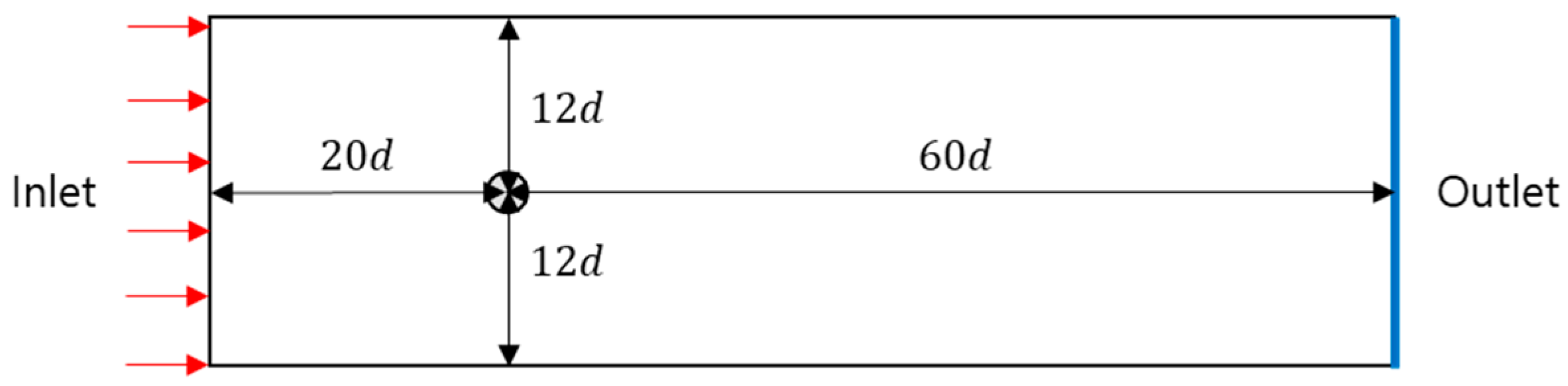
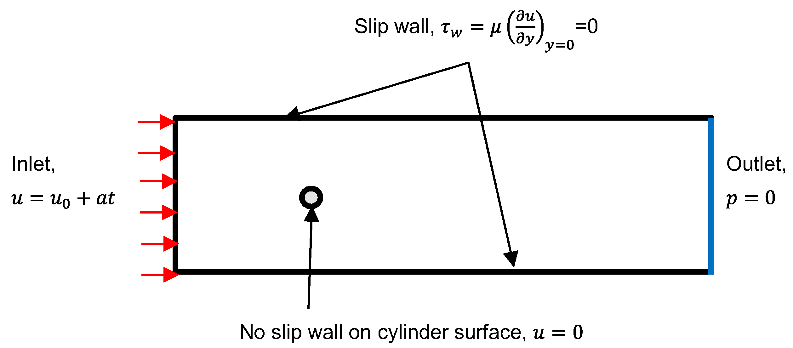
2.2. Computational Domain and Boundary Conditions

The schematic views of a 2D circular cylinder and relevant boundary conditions are shown in Figure 1. The computational domain was determined considering the study of Fackrell [17]. Figure 1 illustrates the computational domain of size of 20 d × 80 d with a cylinder of diameter, d = 0.0127 m. The distance from the center of cylinder to inlet and outlet were set to 20 d and 60 d , respectively, while the distance of 12 d from the center of the circular cylinder to the side walls was set.
The boundary conditions of the numerical model are shown in Figure 2. A uniform velocity was imposed on the inlet of the domain with constant acceleration; a 0-Pa condition was defined at the outlet. The no-slip condition was imposed on the surface of the body, and the slip wall was applied on the side walls, where u 0 is the initial velocity, t is the time, τ w is the wall shear stress, y is the distance from the side wall. As the inflow velocity increases with time, the inflow becomes turbulent from laminar due to flow instability; however, the turbulence was not modeled in the inflow by considering the uniformity of inflow.
As described in Figure 3, the fluid was initially allowed to achieve a steady flow and was then accelerated. The inflow boundary condition was defined by a user-defined function.

2.3. Validation of the Present Method

In order to validate the method employed in this study, the results were compared with the experimental results of Sarpkaya and Garrison [16], in which a vertical water tunnel with a quick-release bottom gate was constructed to obtain a unidirectional, constant flow of fluid over a fixed circular cylinder. The experiments were conducted for the acceleration range of 0.155–0.994g. In this study, the fluid properties were set to a density of 998.2 kg/ m 3 and a kinematic viscosity of 0.001003 kg/m- s .

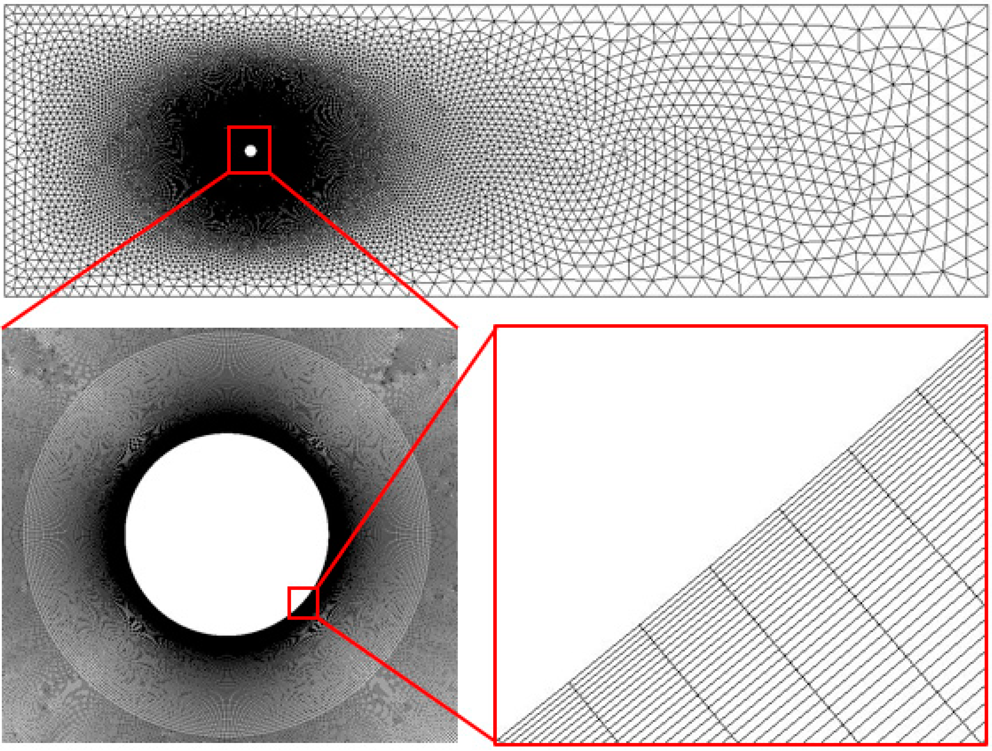
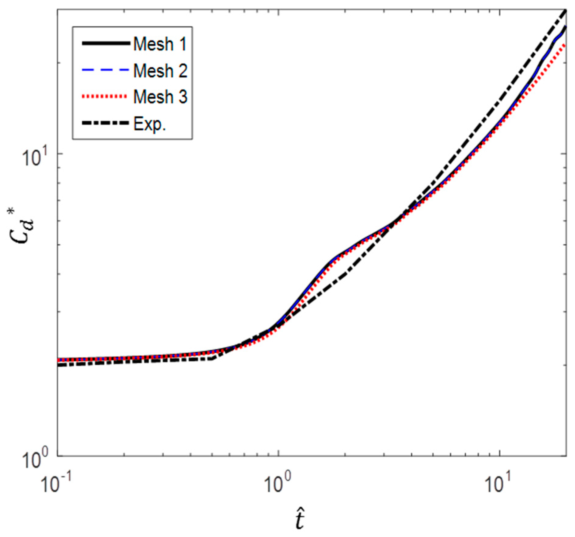
2.3.1. Grid Convergence

In the flow analysis around the bluff body, high gradients are formed along the surface of the cylinder. Therefore, it is important to set the grid around the cylinder adequately. In addition, considering the time required for computational analysis, an appropriate total number of grids should be used, and it is common to set the grids slightly far away from the cylinder. Therefore, as shown in Figure 4, the grid around the cylinder was finely modeled using hexahedra, and the other regions are coarsely modeled using tetrahedra. The computational grid was constructed to calculate the laminar region near the wall, and thus the y + value was close to one.
Three cases of grid configurations, listed in Table 1, were used to determine the appropriate grid size and distribution. To consider the importance of the height of the first cells next to the circular cylinder wall, Mesh 2 was modeled such that y + = 1, and Meshes 1 and 3 were modeled with y + values less than and greater than 1, respectively. At this time, Mesh 3 was modeled such that the total number of grids and the number of grids around the cylinder were greater than those of Mesh 2 to determine the effect of the height of the first layer.
Figure 5 shows the variation in drag coefficient with nondimensional time, compared to the experimental results of Sarpkaya and Garrison [16]. The acceleration given here is a = 9.81 m/s2 and the drag coefficient is defined as
C d * = F d a ρ A
where F d is the drag force per unit length, and A is the area of the circular cylinder.
Keulegan and Carpenter [11] reported that the drag coefficient in a flow with constant acceleration correlated with the relative dimensionless displacement and was not function of time or Reynolds number. Based on this, Sarpkaya and Garrison [16] proposed an analysis using a relative displacement of s/d = 0.5at2/d where s is the displacement of the fluid flow. In this study, for a more intuitive understanding, it was denoted as a nondimensional time t ^ , defined as
t ^ = a t 2 2 d = ( u u 0 ) t 2 d
As can be seen from Figure 5, Mesh 3 case with the largest first grid height deviates the most from the experimental results. When the first grid height is decreased by 2.9 ×   10 6 m, the C d * value is closer to the experimental result than in the case of Mesh 3. However, decreasing the first grid height further by 1.9 ×   10 6 m does not affect the results. Mesh 2 is then selected for the simulations to ensure that the high velocity gradients are resolved and to reduce the computational cost. In Mesh 2, y + = 1 was satisfied for all cases studied, including the most critical case of a/g = 1 at t ^ = 10 .

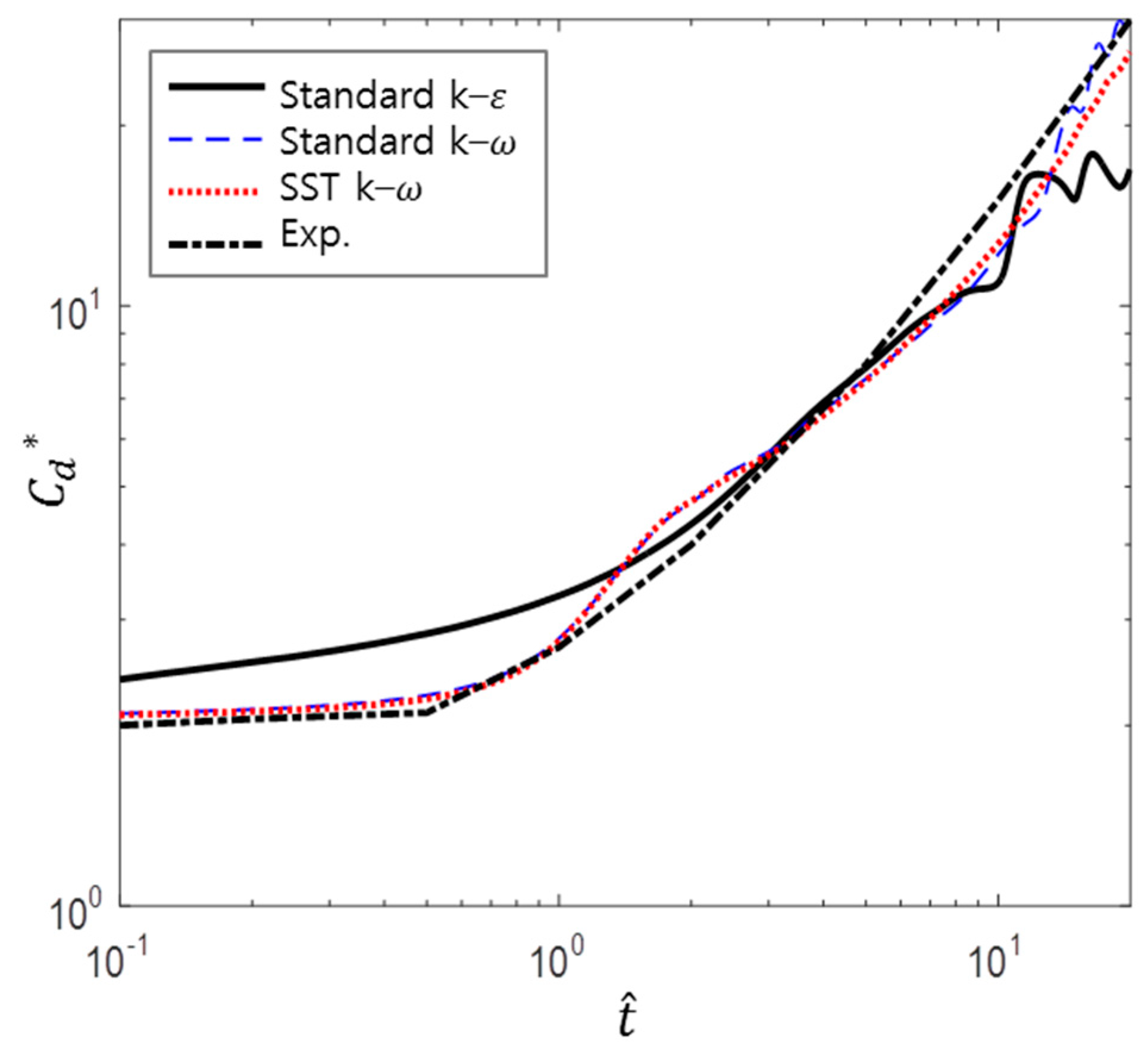
2.3.2. Choice of Turbulence Model

If a bluff body is immersed in a flow with constant acceleration, the surrounding flow enters the turbulent region as the velocity increases. The method used to simulate the turbulence of the unsteady state has a crucial effect on the analytical accuracy.
The most common methods to analyze turbulent flow are is the direct numerical simulation (DNS), the large eddy simulation (LES) and the Reynolds-averaged Navier–Stokes (RANS) equation approach. DNS numerically solves the Navier–Stokes equations without the use of a turbulence model. Using DNS, it is possible to obtain results that are relatively close to actual phenomena with the cost of a large amount of computing resources. LES also enables simulation of real phenomena with sufficient accuracy but requires a large amount of computational resources since it resolves directly large eddies while small eddies are modeled. On the other hand, RANS in general models turbulence of all the scales and offers relatively reasonable results, which saves the computational. In these perspective, this study employs RANS in order for higher computational efficiency with less requirement for resources, and we consider the k–ε model, standard k–ω model, and SST k–ω model among the two-equation models of RANS.
In order to determine the two-equation model for this study, the drag coefficients computed by using different models were compared with experimental data, and the results are shown in Figure 6. In the case of the k–ε model, the initial value of C d * is closer to 2.3 upon inspection. This deviates from the experimental results; thus, this model cannot be used. Furthermore, the k–ε model and standard k– ω model show that vortex shedding occurs in the early stage of the simulation, whereas the SST k–ω model does not. In addition, Sarpkaya’s experimental results do not indicate vortex shedding, and hence these models are unrealistic. The remaining model, the SST k–ω model, shows excellent agreement with only a slight difference at larger values of t ^ ; hence, this model is considered applicable and chosen as the turbulence model.

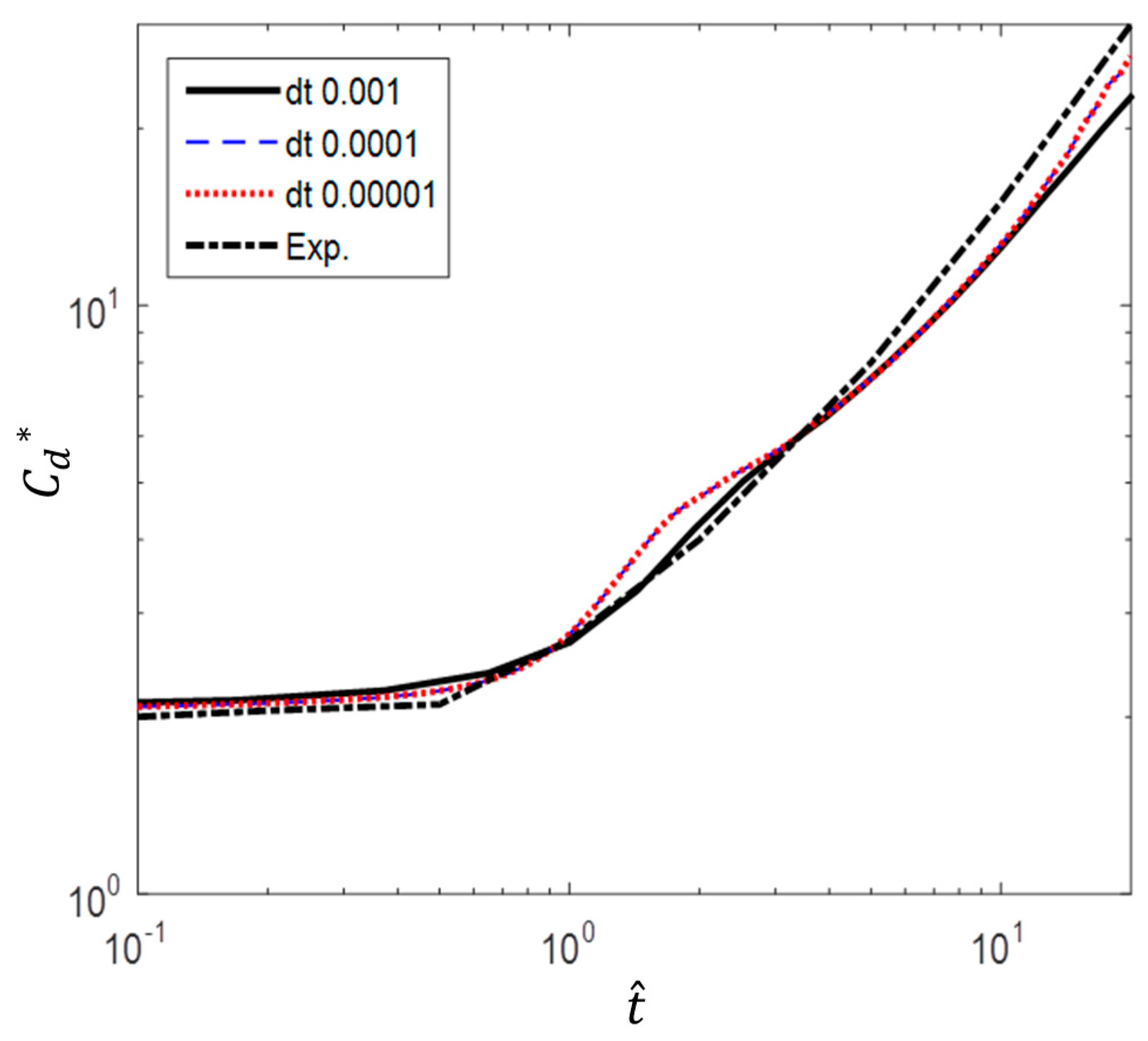
2.3.3. Time Step Convergence

In order to determine the time step size, three different values of 0.001 s, 0.0001 s and 0.00001 s were considered. Figure 7 shows the comparison of the computed drag coefficients with experimental data. Both results with the time step of 0.0001 s and 0.00001 s show that C d * is closer to the experimental data while the result with 0.001 s depicts larger discrepancy. And it was found that the fluid particles were not allowed to pass more than one cell with the time step size of 0.0001s, including the most critical case of a/g = 1 at t ^ = 10 . Therefore, the time step size of 0.0001s was selected for this study.

2.4. Scope of Study

The fluid is initially allowed to achieve a fully developed flow at R e = 40 and 1000 and is then accelerated with the accelerations of 0.0981–9.81 m/s2 as listed in Table 2. The Reynolds number, R e is defined as
R e = ρ v d μ
For a low Reynolds number ( R e = 40), the flow is steady and symmetric, and the wake is laminar, whereas for a high Reynolds number ( R e = 1000), the flow is unsteady, and the vortex street is fully turbulent. However, in the case of high initial velocity ( R e 0 = 1000), only the three accelerations of a = 9.81, 0.981, and 0.4905 m/s2 are studied. Fackrell [17] extended the study on unidirectional constant acceleration of an initial stationary fluid to include a flow with a small initial velocity ( R e 0 < 40), and the case of low Reynolds number in this study was set with reference to this.

3. Drag in Accelerated Flow at Low Initial Velocity

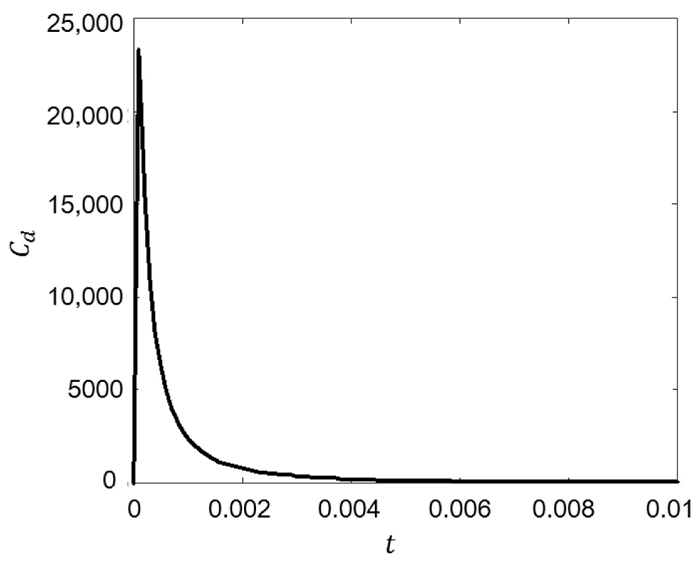
3.1. Overshoot of Drag Force

Figure 8 shows the drag coefficient versus Reynolds number when the flow is accelerated with a = 9.81 m/s2 from the initial constant velocity ( R e 0 = 40). When the flow accelerated, an overshoot phenomenon of the fluid force is evident. The drag coefficient C d is defined as
C d = F d 1 2 ρ v 2 A
The value of C d reached 23,320, which is much greater than that if the motion was steady. However, the C d values constantly decreased after overshoot. A comparison of C d values of non-accelerated and accelerated flow for various acceleration ranges is presented in the following section.

3.2. Difference between Non-Accelerated and Accelerated Flow

In Section 2.3, the computational modeling and numerical methods were verified via comparison with the experimental results of Sarpkaya and Garrison [16]. Based on this, the fluid force was analyzed with varying ranges of acceleration from the low initial velocity ( R e 0 = 40).
Figure 9 shows a comparison between the drag C d of a circular cylinder obtained experimentally by Bullivant [20] and that obtained numerically in this study. The experimental result was measured when the flow was fully developed with constant velocity at each Reynolds number. In contrast, the numerical results describe the instantaneous fluid force during acceleration.
As shown in Figure 9, the drag of accelerated flow is higher than that of non-accelerated flow. The difference between accelerated and non-accelerated flow decreases as the acceleration decreases. In the cases of a/g = 1 and 0.5, the drag steadily decreased, except in the ranges of 30,000 R e 50,000 and 15,000 R e 40,000, respectively, where a constant value was maintained for some time. In the cases of a/g = 0.1, 0.5, and 0.01, the supercritical region observed at a high Reynolds number in the case of steady flow was also found for the ranges of 6000 R e 10,000, 4000 R e 6000, and 1300 R e 1800, respectively. Moreover, except in this region, the drag constantly decreased regardless of whether the region was subcritical or critical. In Figure 9, R e 0 is the Reynolds number defined with the initial velocity.

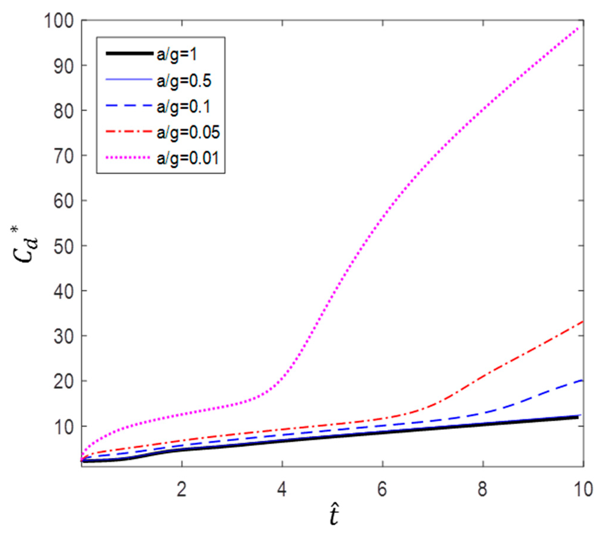
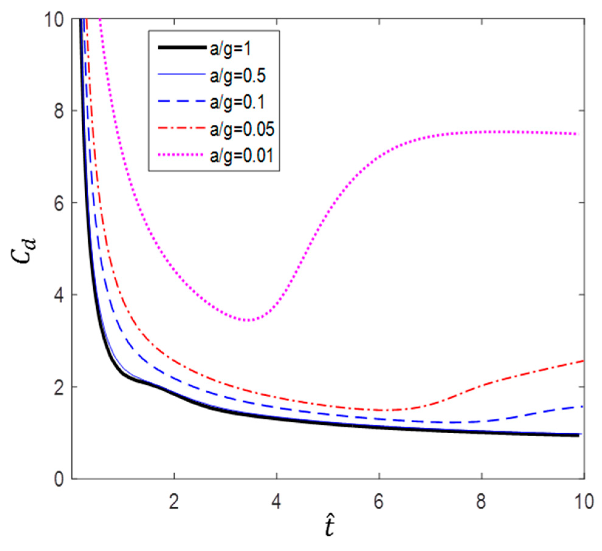
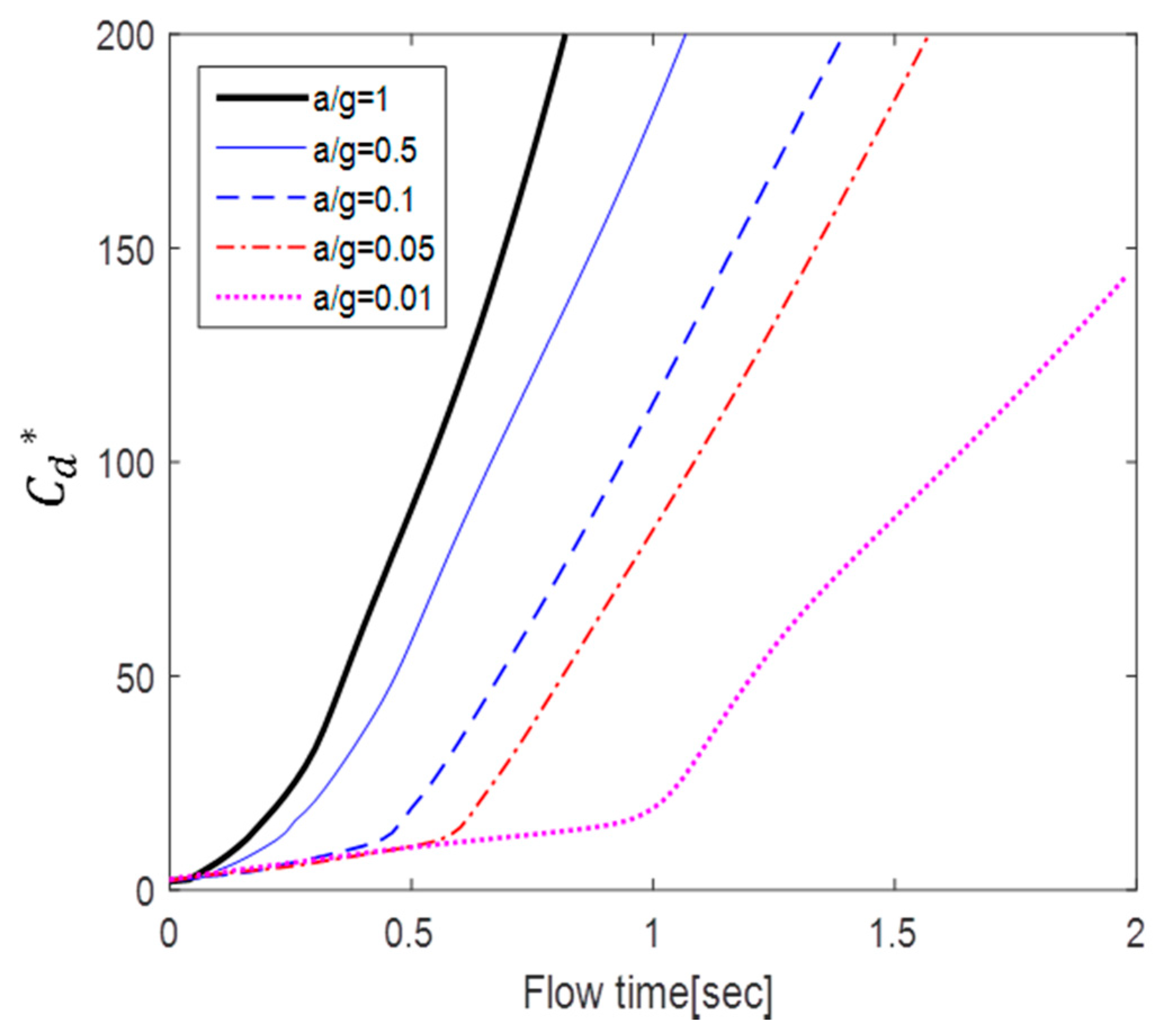
3.3. Drag Changes over Dimensionless Time and Flow Time

According to Figure 10, Figure 11 and Figure 12, the C d value of a circular cylinder immersed in accelerated flow increases while C d * decreases with t ^ and R e . This is because C d is dimensioned by a square term of the velocity and the denominator of C d * contains an acceleration term. At the same time, the fluid force F increases over time. Therefore, the drag coefficient varies greatly according to the dimensionless method; in this paper, C d or C d * is used as necessary.
As mentioned earlier, Sarpkaya and Garrison [16] proved that there is a correlation among drag coefficients   ( C d * ) in terms of dimensionless distance (s/d), and Fackrell [17] also showed that correlation among the data was very good for a/g = 1, 0.5, and 0.2. In this study, we found that the correlation of the data is good for a/g = 1 and 0.5. However, as can be seen in Figure 10, for a/g = 0.1, 0.05, and 0.5, the gradient of C d * increases as the acceleration decreases. Furthermore, Figure 11, which shows the variation in C d according to dimensionless time.
According to Figure 10 and Figure 11, a lower acceleration results in larger C d   at the same dimensionless time. However, more flow time is required to achieve the same change in dimensionless time with lower accelerations. For example, the case of a/g = 10 takes 10 times longer to achieve the flow time of the case of a/g = 1. Figure 12 shows the variation in C d * with flow time t. The results show that the smaller the acceleration, the smaller the value of C d * . In addition, the inflection point at which the slope increases sharply is shown in the cases of a/g = 0.1, 0.05, and 0.01.

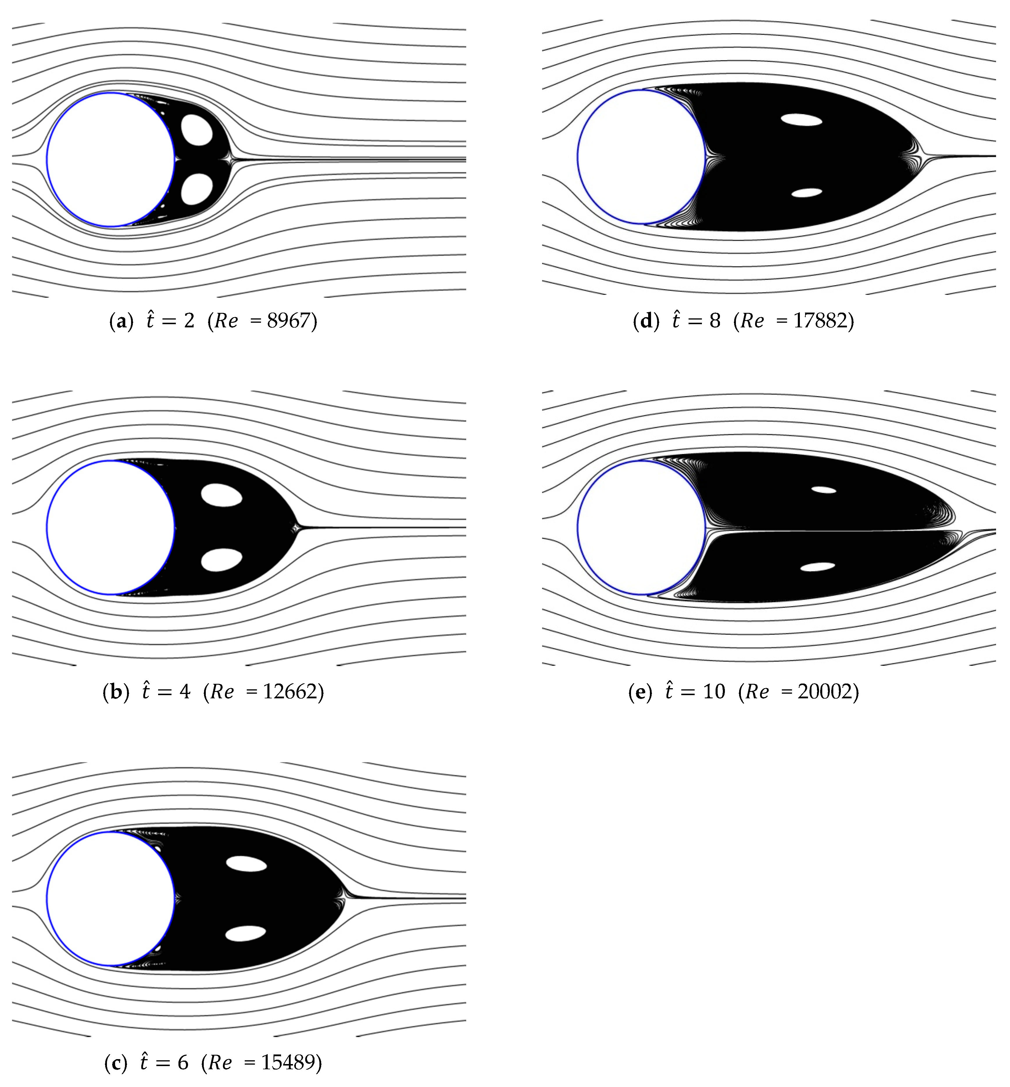
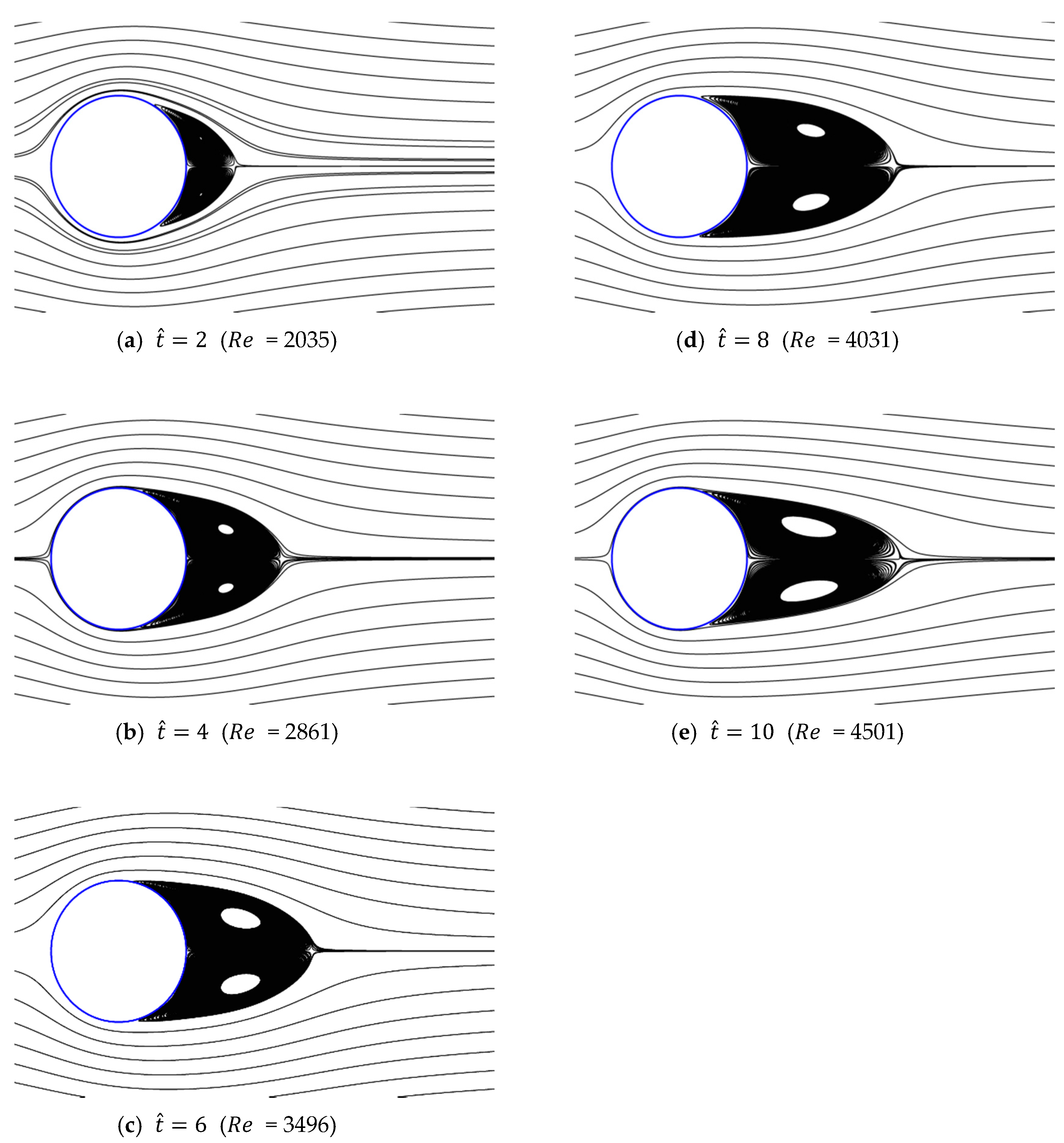
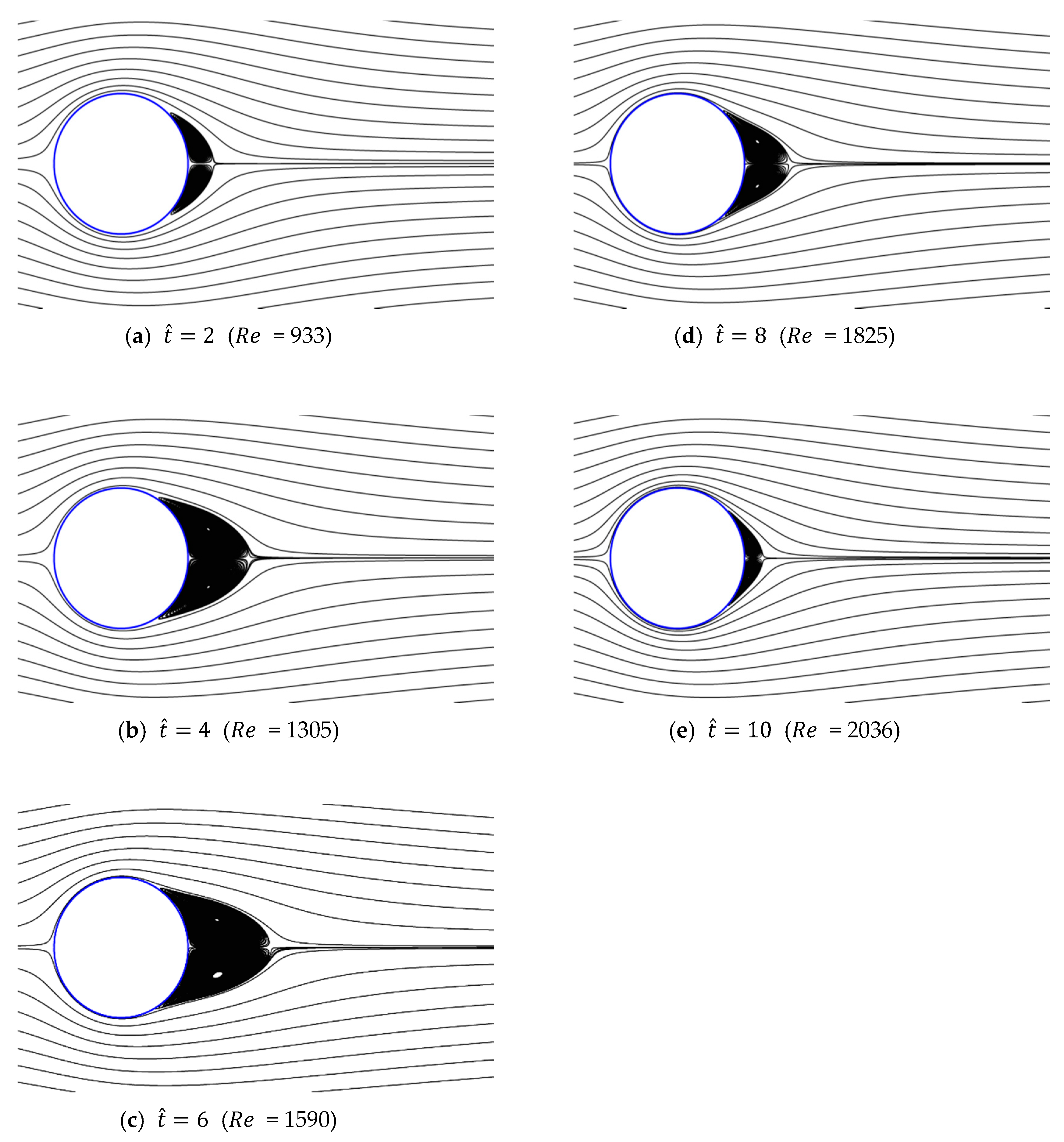
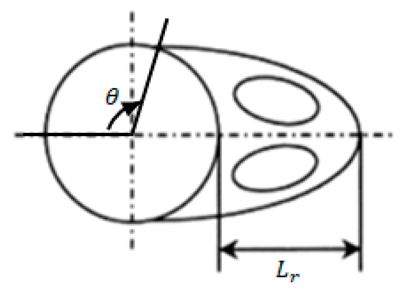
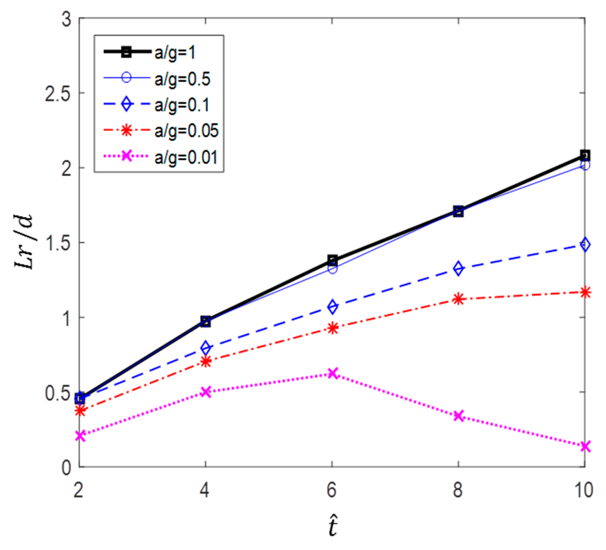
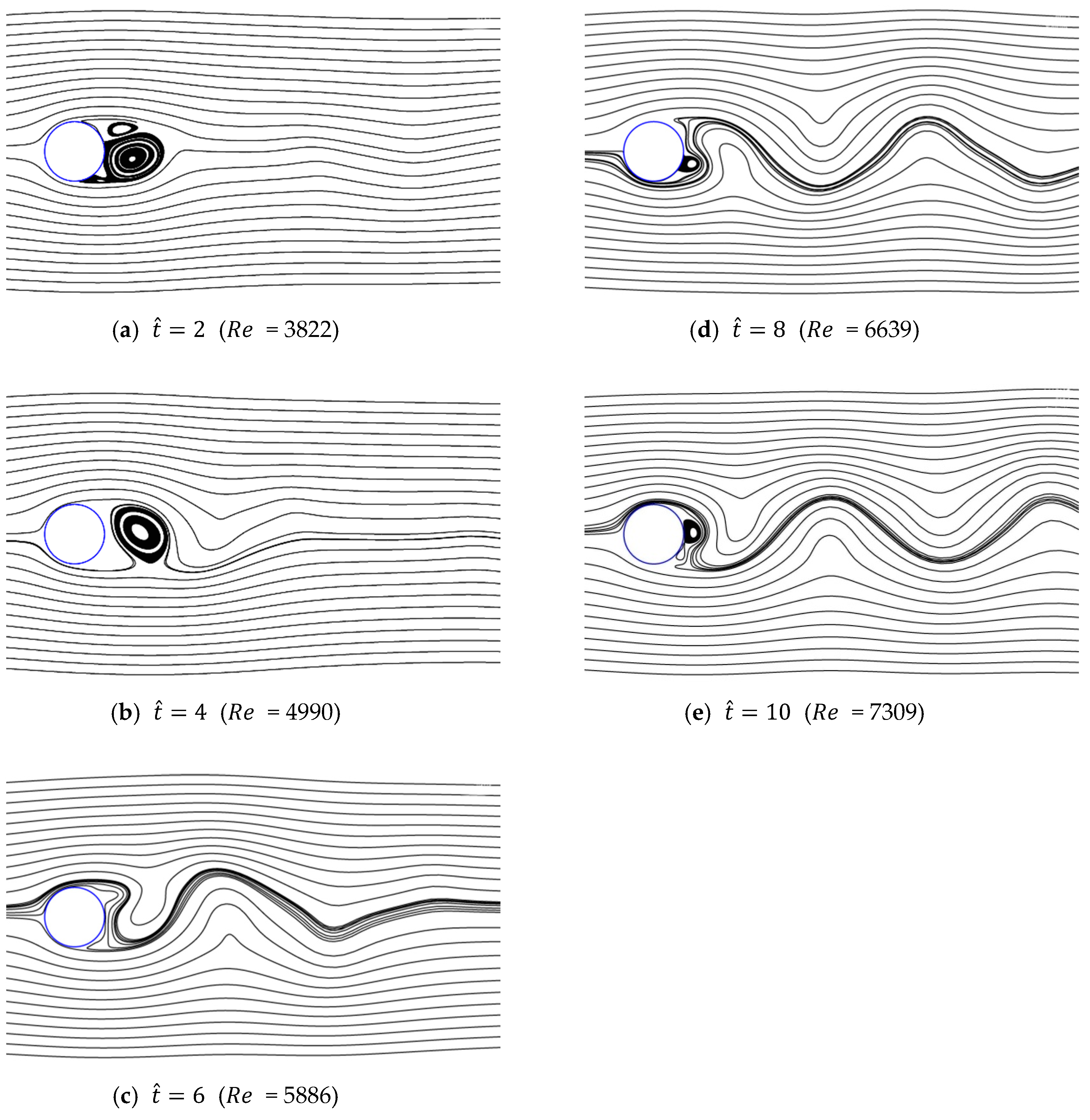
3.4. Vortex Formation and Development

Figure 13, Figure 14, Figure 15, Figure 16 and Figure 17 show the streamlines for various values of t ^ and a/g. If the circular cylinder is immersed in unidirectional constant flow with a high Reynolds number, the symmetrical pattern becomes unstable and vortex shedding occurs behind the cylinder. In the case of accelerated flow, as the velocity increases, the vortex forms and grows, but vortex shedding does not appear. These results are consistent with Sarpkaya and Garrison’s [16] experiment, which showed no vortex shedding in the range of t ^ < 30. This indicates that even if the Reynolds number of the fully developed steady flow and that of the accelerated unsteady flow match instantaneously, the wake situation behind the object at that moment is different. The size of the vortex tends to increase as the dimensionless time increases because the energy generated by acceleration contributes to the increasing size of the vortex. In addition, as the dimensionless time increases, the length of the recirculation length gradually grows, except for the case of a/g = 0.01, where it starts to dwindle at t   ^ = 6 . Furthermore, as per the correlation between the drag coefficients, shown in Figure 10 and Figure 11, respectively, for the cases of a/g = 1 and 0.5, the wake shape behind the cylinder according to t ^ is very similar.
The recirculation length and separation angle are closely related to the drag acting on the circular cylinder and are a part of the criteria for quantifying the size of the vortices. The recirculation length and separation angle are defined as L r and θ , as shown in Figure 18.
The recirculation length at low Reynolds numbers, in the range of 20 R e 80, has been studied by Acrivos et al. [21]. In this study, vortex shedding did not appear, even at high Reynolds numbers. Therefore, to quantitatively evaluate the size of the vortex, the variation in the recirculation length according to the dimensionless time in each case is shown in Figure 19. The results show that at higher acceleration and dimensionless time, the recirculation length and its rate of increase are greater. In particular, in the cases of a/g = 1 and 0.5, the recirculation length increases linearly with the relative time ( t ^ ), whereas in the cases of a/g = 0.1 and 0.05, its rate of increase was found to decrease. In addition, as shown in Figure 20, the separation angle also increases the size of the vortex by causing it to move in the windward direction along the surface of the cylinder as a/g and t ^ increase. These trends can be seen in Figure 13, Figure 14, Figure 15, Figure 16 and Figure 17. This change in the vortex behind the cylinder is directly related to the variation in C d shown in Figure 11. Ultimately, when the size of vortex is larger, C d is decreased. In the case of a/g = 0.01, the recirculation length decreases after t ^ = 6, and this is considered to influence the recovery of the C d value.

4. Drag in Accelerated Flow at High Initial Velocity

4.1. Difference between Non-Accelerated and Accelerated Flow

In Section 3, the drag characteristics of circular cylinders immersed in flow that is accelerated from a low initial velocity ( R e 0 = 40) were analyzed. In this section, flow accelerated from a high initial velocity ( R e 0 = 1000) is considered. First, various acceleration ranges are examined. Then, the effect of initial velocity on drag change is analyzed in Section 5.
Figure 21 shows the logarithmic distribution of C d obtained experimentally in the case of non-accelerated flow by Bullivant [20] and that obtained numerically in the case of accelerated flow in this study. As evident from Figure 21, the C d values of accelerated flow were higher for all ranges than those of non-accelerated flow. Furthermore, the lower the acceleration, the smaller the difference between the drag values of the accelerated and non-accelerated flows. It is noticeable that C d values of accelerated flow decrease with time and oscillate when approaching the value of the non-accelerated flow in all acceleration ranges. In addition, the supercritical regions did not appear, unlike in the case of low initial velocity.

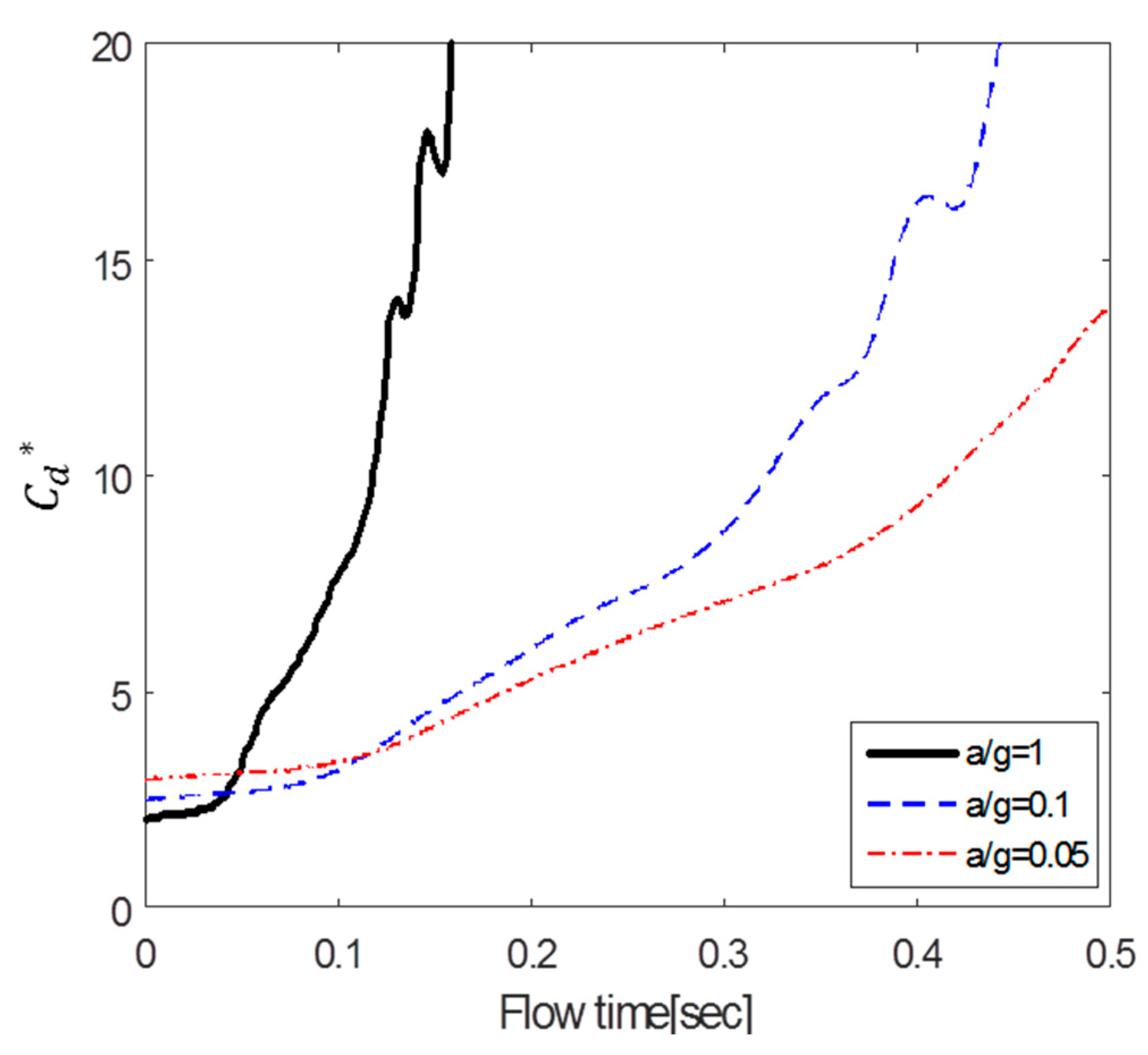
4.2. Drag Changes over Dimensionless Time and Flow Time

Figure 22 and Figure 23 show the variations in C d * and C d , respectively, with t ^ . As mentioned earlier, it was confirmed that the results for several different accelerations showed good correlation in the case of low initial velocity. In the high initial velocity cases, it can be seen that the C d * and C d values correlated well with respect to dimensionless time.
Figure 24 illustrates the variation in C d * with time. The results show that the smaller the acceleration, the smaller the value of C d * . The inflection point at which the slope increases sharply appears in the case of a/g = 1 only.

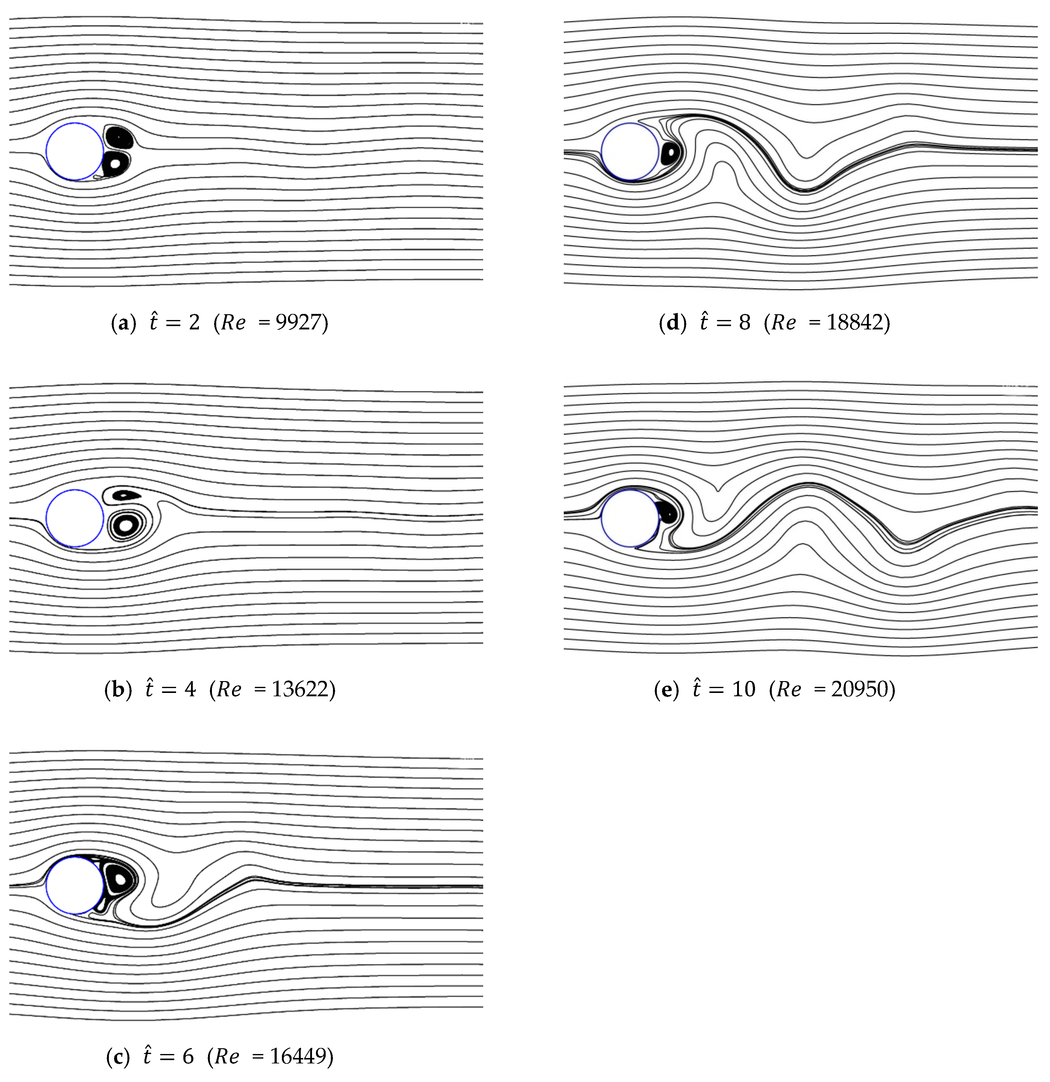
4.3. Vortex Shedding Formation Development

Figure 25, Figure 26 and Figure 27 show the streamlines for various values of t ^ and a/g. As shown previously, in the case of low initial velocity, the size of symmetrical vortices tends to increase as the dimensionless time is increased. In contrast, in the case of high initial velocity, asymmetrical pair vortices are generated at the beginning, and the vortex is then created and destroyed alternately. Vortex shedding also gradually develops as time passes. Because of the growth of this wake, the supercritical region is not shown, but C d rapidly approaches the drag of the non-accelerated flow with oscillations, as shown in Figure 21.

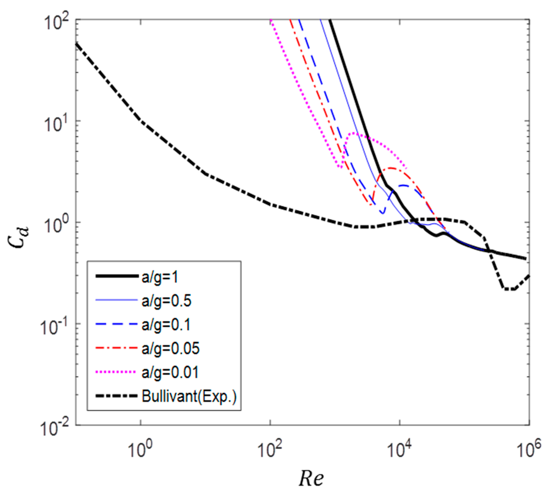
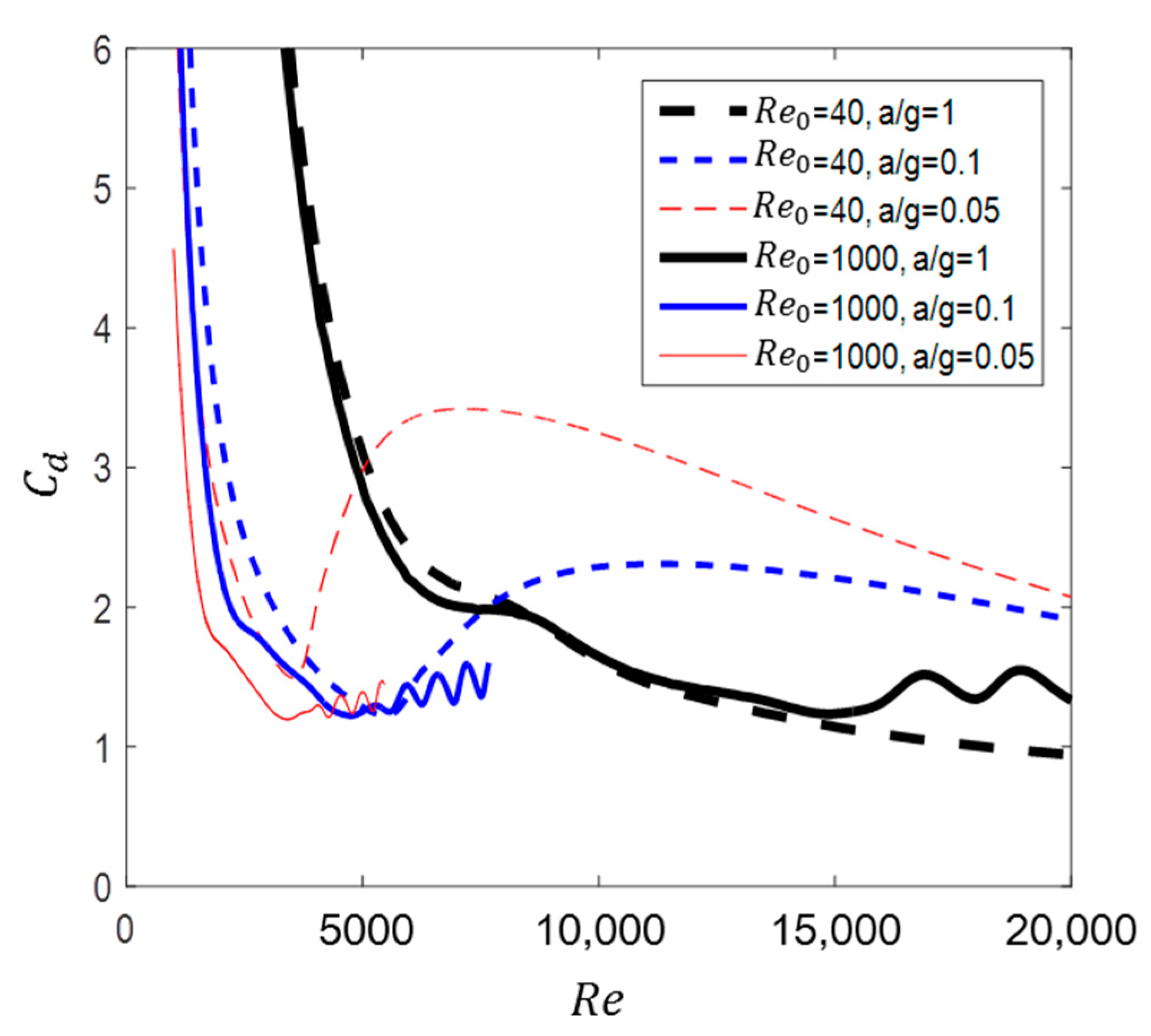
5. Comparison of Fluid Force by Initial Velocity

Thus far, the fluid forces for two initial velocities have been analyzed with respect to several accelerations. Figure 28 presents the effect of the initial state of flow past a circular cylinder on the drag change. When the flow is accelerated at R e 0 = 40 , the supercritical region is prominent due to the variation in the vortex size. In contrast, in the case of R e 0 = 1000 , the oscillation of C d occurred due to the generation and development of vortex shedding. As a result, the influence of the initial state is transmitted even when the acceleration continues, which eventually leads to a difference in the drag between the two initial velocities.
The formation of vortex shedding is evident from the variation in lift coefficient with Reynolds number, as shown in Figure 29. The lift coefficient C l was defined as follows:
C l = F l 1 2 ρ v 2 A
where F l is the lift force per unit length. In the case of R e 0 = 40, C l converged to 0. In the case of R e 0 = 1000, the value of C l varied due to vortex shedding, and the amplitude also increased with time.

6. Conclusions

In this study, the effects of accelerated flow on a 2D bluff body were analyzed numerically. To investigate the drag increase and its relationship with the form and development of the wake behind the cylinder, this study employed a finite-volume based computational fluid dynamics method using Fluent 19.2 with the SST k–ω model for turbulence effects.
Fackrell [17] showed that good correlation among results was achieved when using dimensionless parameters in the limited range of acceleration at a/g = 0.2, 0.5 and 1.0 with the low initial Reynolds number used. This study extended the scope of the investigation by considering different initial Reynolds numbers ( R e 0 = 40 and 1000) and the acceleration range was extended to 0.01–1.0g.
In addition, a dimensionless time t ^ was introduced to aid in intuitive understanding, and the change in drag according to t ^ was analyzed. Because the drag acting on the body and the wake are closely related, the separation angle and the recirculation length were investigated. The numerical results obtained are summarized as follows:
(1) The results show that the initial drag increases due to overshoot, and that the drag decreases as dimensionless time increases. In addition, the calculated drag in this study is in good agreement with that from previous studies, clearly showing an increase in comparison with the drag in the flow with constant velocity.
(2) The value of C d decreases as R e and t ^ increase, whereas the value of C d   * increases as R e and t ^ increase. When C d * is expressed over time t, the inflection point at which the slope increases sharply is observed. The results also show that the smaller the acceleration, the smaller the value.
(3) As in the previous study, it was confirmed that the correlation of data is good for a/g = 1 and 0.5, but in the case of a/g = 0.1, 0.05, and 0.01, where the flow is relatively steady, the value of C d   * increases.
(4) In the case of the low initial Reynolds number, as the acceleration and t ^ increase, the recirculation length gradually increases, and the recirculation length decreases after t ^ = 6 only when a/g = 0.01. Similarly, the separation location moves toward the windward direction along the surface of cylinder, which results in the increase of the size of the vortex as the acceleration and t ^ increase. This variation in the size of the vortex behind the cylinder is directly related to the C d ; when the size of vortex is larger, C d is decreased.
(5) In the case of the high initial Reynolds number, an asymmetrical pair of vortices is generated at the beginning. Then, the vortex is created and destroyed alternately. Vortex shedding also gradually develops with time. Due to the growth of this wake, the supercritical region is not shown, but C d rapidly approaches the value of the non-accelerated flow with oscillations.
(6) In the case of a low initial Reynolds number, vortex shedding does not occur, but the supercritical region is prominent due to the variation in the vortex size, whereas in the case of a high initial Reynolds number, the drag force fluctuates due to the generation and development of vortex shedding. This shows that the influence of the initial Reynolds number propagates in the accelerated flow, resulting in a change in the fluid force.
As a final remark, the drag force in an accelerated flow field over a stationary circular cylinder is considerably different from that in a constant velocity flow field at the same Reynolds number. Therefore, the load evaluation of the bluff body in an accelerated flow must be considered based on the unsteady state conditions.

Author Contributions

Conceptualization, H.A.S. and S.L.; methodology, H.A.S. and S.L.; software, H.A.S. and S.L.; validation, H.A.S.; formal analysis, H.A.S.; investigation, H.A.S., S.L., and J.L.; resources, H.A.S., S.L., and J.L.; data curation, H.A.S. and S.L.; writing—original draft preparation, H.A.S. and S.L.; writing—review and editing, H.A.S. and S.L.; visualization, H.A.S. and S.L.; supervision, S.L.; project administration, S.L.; funding acquisition, S.L. All authors have read and agreed to the published version of the manuscript.

Funding

This research was funded by a grant (2018-MOIS31-009) from Fundamental Technology Development Program for Extreme Disaster Response funded by Korean Ministry of Interior and Safety(MOIS).

Conflicts of Interest

The authors declare no conflict of interest.

References

  1. Nomura, T.; Kitamura, N.; Kitagawa, T. Characteristics of unsteady drag on a square cylinder under sudden change of wind speed. In Proceedings of the 3rd International Symposium on Computational Wind Engineering (CWE 2000), Birmingham, UK, 4–7 September 2000. [Google Scholar]
  2. Matsumoto, M.; Shimamura, M.; Maeda, T.; Shirato, H.; Yagi, T. Drag forces on 2-D cylinders due to sudden increase of wind velocity. In Proceedings of the 12th International Conference on Wind Engineering, Cairns, Australia, 1–6 July 2007; pp. 1727–1734. Available online: https://www.tib.eu/en/search/id/TIBKAT%3A661555100/12th-International-Conference-on-Wind-Engineering/ (accessed on 20 November 2019).
  3. Takeuchi, T.; Maeda, J. Effects of inertia force proportional to flow acceleration on unsteady wind forces acting on an elliptic cylinder under short-rise-time gusts. In Proceedings of the 5th International Symposium on Computational Wind Engineering, Chapel Hill, NC, USA, 23–27 May 2010; Available online: https://www.jstage.jst.go.jp/article/kazekosymp/21/0/21_0_185/_article/-char/en (accessed on 10 October 2019).
  4. Rho, J.; Lee, Y.; Kim, K.H.; Lee, D.H.; Cho, H.K. Experimental studies on aerodynamic characteristics in unsteady accelerated flow. In Proceedings of the Spring Conference of the Korean Society for Aeronautical & Space Sciences, Seoul, Korea, February 2008; pp. 582–585. Available online: http://www.dbpia.co.kr/journal/articleDetail?nodeId=NODE01116210 (accessed on 29 May 2019).
  5. Lee, Y.; Rho, J.; Kim, K.H.; Lee, D.H. Wind tunnel test of the aerodynamic characteristics around a circular and square cylinders in unsteady accelerated flow. In Proceedings of the Spring Conference of The Korean Society for Aeronautical & Space Sciences, Daejun, Korea, February 2009; pp. 78–81. Available online: http://www.dbpia.co.kr/journal/articleDetail?nodeId=NODE01203450 (accessed on 29 May 2019).
  6. Lee, Y.; Rho, J.; Kim, K.H.; Lee, D.H. Fundamental studies on free stream acceleration effect on drag force in bluff bodies. J. Mech. Sci. Technol. 2011, 25, 695–701. [Google Scholar] [CrossRef]
  7. Mason, M.S.; Yang, T. Modulation of vortex induced crosswind forces on a square cylinder during accelerating flow. In Proceedings of the 20th Australasian Fluid Mechanics Conference, Perth, Australia, 5–8 December 2016; Available online: https://people.eng.unimelb.edu.au/imarusic/proceedings/20/639%20Paper.pdf (accessed on 11 June 2019).
  8. Lamb, H. Hydrodynamics, 6th ed.; Dover Publications: New York, NY, USA, 1945. [Google Scholar]
  9. Birkhoff, G. Chapter 6: Added Mass. In Hydrodynamics: A Study in Logic, Fact, Similitude; Princeton University Press: Princeton, NJ, USA, 1960. [Google Scholar]
  10. Yih, C.S. Fluid Mechanics: A Concise Introduction to the Theory; West River Press: New York, NY, USA, 1969. [Google Scholar]
  11. Keulegan, G.H.; Carpenter, L.H. Forces on cylinders and plates in oscillating fluid, United States Bureau of Standards. J. Res. 1958, 60, 423–440. [Google Scholar]
  12. Patton, K.T. Tables of hydrodynamic mass factors for translational motion. In American Society of Mechanical Engineers—Meeting WA/UNT-2; ASME: New York, NY, USA, 1965. [Google Scholar]
  13. Kennard, E. Irrotational Flow of Frictionless Fluids: Mostly of Invariable Density; Report 2299; David Taylor Model Basin: Washington, DC, USA, 1967. [Google Scholar]
  14. Brennen, C.E. A Review of Added Mass; Fluid Inertial Forces; Report CR 82.010; Naval Civil Engineering Laboratory: Port Hueneme, CA, USA, 1982. [Google Scholar]
  15. Sarpkaya, T. Lift, drag, added-mass coefficients for circular cylinder immersed in time-dependent flow. J. Appl. Mech. 1962, 30, 13–15. [Google Scholar] [CrossRef]
  16. Sarpkaya, T.; Garrison, C.J. Vortex formation and resistance in unsteady flow. J. Appl. Mech. 1963, 30, 16–24. [Google Scholar] [CrossRef]
  17. Fackrell, S. Study of the Added Mass of Cylinders and Spheres. Ph.D. Thesis, University of Windsor, Windsor, ON, Canada, 2011. Available online: https://scholar.uwindsor.ca/cgi/viewcontent.cgi?article=1457&context=etd (accessed on 25 January 2018).
  18. Benim, A.C.; Pasqualotto, E.; Suh, S.H. Modeling turbulent flow past a circular cylinder by RANS, URANS, LES and DES. Progress Comput. Fluid Dyn. Int. J. 2008, 8, 299–307. [Google Scholar] [CrossRef]
  19. Liuliu, S.; Yang, G.; Yao, S. Large eddy simulation of flow past a square cylinder with rounded leading corners: A comparison of 2D and 3D approaches. J. Mech. Sci. Technol. 2018, 32, 2671–2680. [Google Scholar]
  20. Bullivant, W.K. Test of the NACA 0025; 0035 Airfoils in the Full Scale Wind Tunnel; NACA Technical Report 708; NACA: Langley Field, VA, USA, 1941; Available online: https://digital.library.unt.edu/ark:/67531/metadc66369/m1/1/ (accessed on 1 April 2020).
  21. Acrivos, A.; Leal, L.G.; Snowden, D.D.; Pan, F. Further experiments on steady separated flows past bluff objects. J. Fluid Mech. 1968, 34, 25–48. [Google Scholar] [CrossRef]
Figure 1. Schematic views of the computational domain.
Water 12 01790 g001
Figure 2. Boundary conditions.
Water 12 01790 g002
Figure 3. Inflow boundary condition.
Water 12 01790 g003
Figure 4. Mesh in the computational domain.
Water 12 01790 g004
Figure 5. Comparison of different grid configurations (experimental data from Sarpkaya and Garrison [16]).
Water 12 01790 g005
Figure 6. Comparison of different turbulence models (experimental data from Sarpkaya and Garrison [16]).
Water 12 01790 g006
Figure 7. Comparison of different time steps (experimental data from Sarpkaya and Garrison [16]).
Water 12 01790 g007
Figure 8. Overshoot phenomenon of drag force.
Water 12 01790 g008
Figure 9. Comparison of drag coefficient C d between non-accelerated flow (Bullivant [20]) and accelerated flow ( R e 0 = 40 ).
Water 12 01790 g009
Figure 10. Dimensionless time variation of drag coefficient C d * ( R e 0 = 40 ).
Water 12 01790 g010
Figure 11. Dimensionless time variation of drag coefficient C d ( R e 0 = 40 ).
Water 12 01790 g011
Figure 12. Temporal variation of drag coefficient C d * ( R e 0 = 40 ).
Water 12 01790 g012
Figure 13. Streamlines around circular cylinder (a/g = 1, R e 0 = 40 ).
Water 12 01790 g013
Figure 14. Streamlines around circular cylinder (a/g = 0.5, R e 0 = 40 ).
Water 12 01790 g014
Figure 15. Streamlines around circular cylinder (a/g = 0.1, R e 0 = 40 ).
Water 12 01790 g015
Figure 16. Streamlines around circular cylinder (a/g = 0.05, R e 0 = 40 ).
Water 12 01790 g016
Figure 17. Streamlines around circular cylinder (a/g = 0.01, R e 0 = 40 ).
Water 12 01790 g017
Figure 18. Definition of recirculation length and separation angle.
Water 12 01790 g018
Figure 19. Recirculation length versus t ^ for various accelerations.
Water 12 01790 g019
Figure 20. Separation angle versus t ^ for various accelerations.
Water 12 01790 g020
Figure 21. Comparison of drag coefficient C d between non-accelerated flow (Bullivant [20]) and accelerated flow ( R e 0 = 1000 ).
Water 12 01790 g021
Figure 22. Dimensionless time variation of drag coefficient C d * ( R e 0 = 1000 ).
Water 12 01790 g022
Figure 23. Dimensionless time variation of drag coefficient C d ( R e 0 = 1000 ).
Water 12 01790 g023
Figure 24. Temporal variation of drag coefficient C d * ( R e 0 = 1000 ).
Water 12 01790 g024
Figure 25. Streamlines around circular cylinder (a/g = 1, R e 0 = 1000 ).
Water 12 01790 g025
Figure 26. Streamlines around circular cylinder (a/g = 0.1, R e 0 = 1000 ).
Water 12 01790 g026
Figure 27. Streamlines around circular cylinder (a/g = 0.05, R e 0 = 1000 ).
Water 12 01790 g027
Figure 28. C d versus R e for flow past circular cylinder at two initial velocities
Water 12 01790 g028
Figure 29. C l versus R e for flow past circular cylinder of two different initial velocity.
Water 12 01790 g029
Table 1. Mesh information for grid convergence.
First Grid Height (m)Total Number of GridsNumber of Grids around the Cylinder
Mesh 11.9 ×   10 6 454,012940
Mesh 22.9 ×   10 6 229,211800
Mesh 35.9 ×   10 6 376,6801600
Table 2. Computational cases.
a/g a   ( m / s 2 )
19.81
0.54.905
0.10.981
0.050.4905
0.010.0981

