Article

Seasonal Distributions of Phytoplankton and Environmental Factors Generate Algal Blooms in the Taehwa River, South Korea

1
Marine Environment Research Division, National Institute of Fisheries Science, 216 Gijanghaean-ro, Gijang-eup, Gijang-gun, Busan 46083, Korea
2
Research and Development Planning Division, National Institute of Fisheries Science, 216 Gijanghaean-ro, Gijang-eup, Gijang-gun, Busan 46083, Korea
3
Fisheries Resources and Environment Research Division, South Sea Fisheries Research Institute, 22 Sepodangmeori-gil, Hwayang-myeon, Yeosu 59780, Korea
4
Oceanic Climate and Ecology Research Division, National Institute of Fisheries Science, 216 Gijanghaean-ro, Gijang-eup, Gijang-gun, Busan 46083, Korea
*
Author to whom correspondence should be addressed.
Water 2020, 12(12), 3329; https://doi.org/10.3390/w12123329
Submission received: 27 October 2020 / Revised: 20 November 2020 / Accepted: 24 November 2020 / Published: 26 November 2020
(This article belongs to the Special Issue The Ecological Assessment of Rivers and Estuaries: Present and Future)

Abstract

:
Algal blooms have occurred in the Taehwa River estuary in South Korea despite the improvement of water quality since environmental renewal projects in the 1990s. In this study, we investigated the causes of algal blooms by measuring the water retention time using a floating buoy, water quality parameters, and phytoplankton distribution data from 2012. An algal bloom did not occur in February because of phosphate limitations in the Taehwa River estuary; however, the concentration of nutrients in the water inflow from the basin triggered a significant algal bloom in the upper estuary in the month of May. In this regard, the phytoplankton population was dominated by nano- and pico-sized flagellates. In August, the freshwater inflow into the estuary greatly increased due to heavy rainfall, resulting in a shorter retention time of the water bodies, which seemed to prevent an algal bloom. In November, a bloom of Cryptophyceae occurred at one of the sites (the U2 site) due to sufficient nutrients in the water and the long retention times of the water bodies. Our results indicate that a decrease in the nutrients (N and P) supplied from the basin is required for a reduction in algal blooms in the Taehwa River estuary. Additional studies are needed to further elucidate the effects of the land-based, nutrient-rich pollutants flowing into the Taehwa River estuary on algal bloom generation considering the fact that the streams have different environmental characteristics.

1. Introduction

Algal blooms are generally considered to be a major problem in estuaries and coastal areas worldwide [1,2,3]. Nutrient-rich rivers have begun to flow into estuaries as the world becomes increasingly industrialized and urbanized [4]. After industrialization and urbanization, the influx of anthropogenically introduced nutrients has increased by more than 10 times in recent years [5]. The state of nutrient over-enrichment in the water has caused algal blooms and has led to high primary productivity [6,7]. Algal blooms also enhance the deposition of organic matter [8], which can lead to hypoxia at the water and sediment interface of an estuary and also in the sediments. Such an impact could negatively affect the entire dynamics of the aquatic and benthic ecosystem.
Climate changes have increased the occurrence of harmful algal blooms [9] and the increasing water temperature has resulted in a stronger pycnocline, which affects phytoplankton growth [10]. Because of climate change, a large-scale dinoflagellate bloom broke out in San Francisco Bay in 2004; this type of algal bloom had not occurred for 30 years [11]. Significant ecosystem changes have been observed due to the effect of climate change on various coastal areas [12], the open ocean [13], as well as changes in fishery resources in the Republic of Korea (ROK) [14]. Harmful algal blooms caused by Cochlodinium polykrikoides frequently occur in the southern coastal areas of the ROK in summer [15,16]. Those blooms have extended to the southern and eastern coastal areas due to climate change [17], and increasing solar radiation and water temperature have also given rise to algal blooms during the winter season [18]. Algal blooms have also started to proliferate earlier, with a longer duration than expected and a higher cell density [19].
The study area was conducted in the southern region of Korea located in the middle latitude (33~38° N), and therefore it has four seasons. The climate of ROK is largely characterized by having temperate monsoon with rainy seasons (June—September, especially July—August) and dry seasons (October—May). For this reason, the ecological environment including rivers in ROK has changed significantly. Ulsan city is one of the largest cities in the ROK that is located on the banks of the Taehwa River. The Taehwa River has a length of 47.54 km and flows across the center of the town to discharge into the East Sea. Since the 1960s, Korea has become rapidly industrialized and urbanized. Many industrial complexes have also been constructed around the Taehwa River estuary since the 1960s. After the development of these complexes, various pollutants, originating from raw domestic and industrial sewage, run into the Taehwa River [20,21,22]. As a result, algal blooms frequently occur and fish mass mortality has been occurring in the Taehwa River estuary. Therefore, effective management strategies that decrease the input of nutrients (N, P) into the estuary are needed to decrease the threat of algal blooms in the river [6].
Since the mid-1990s, the Ulsan local government has been investing large sums of money, endeavoring to improve the Taehwa River water quality. Several projects have been undertaken to improve the river environment, including building a sewage treatment plant, connecting a waste pipe, and dredging the stream. As an outcome of these projects, the water quality and ecosystem were improved from a “very poor” grade in 1997 to a “good” grade in 2007 [23]. Although the water quality has improved, the seasonal recurrence of algal blooms is still being observed. Some studies have been conducted on algal blooms in the Taehwa River estuary, with most focusing on the Ulsan Bay (the Taehwa River flows into the Ulsan Bay). The main factors that influence the occurrence of algal blooms are considered to be precipitation and flow rate [24], small streams, and sewage drains connected to the Taehwa River [25]. These studies mainly focused on algal blooms in the Taehwa River that occur in the winter. Algal blooms that were mainly dominated by non-toxic cryptomonads occurred in the Taehwa River during the dry season (November to April [26]). Other studies suggest that algal blooms may also occur during the winter season, although algal bloom outbreaks mainly occur during the spring and summer seasons [25]. The objective of this study is to analyze the causes of seasonal algal blooms by evaluating key water characteristics based on the physical environment. The results of this study could provide useful data for maintaining and preserving a healthy ecological system in the Taehwa River estuary.

2. Materials and Methods

We conducted surveys from the Taehwa River estuary to the mouth of the Ulsan Bay (Figure 1). There were twelve sampling stations from the upper section of the estuary (U1) to Ulsan Bay (U12); these were the same sites as a previous study on the sedimentary environment of the Taehwa River estuary [27]. U1 is located near the old Samho Bridge and is connected to the Mugeot stream. U2 is located near the Taehwa River national garden, and U3 is located in Ulsan Park that surrounds the garden. U4 is located near the Beonyeong Bridge. U5 is located before the Dong River joins to the Thaehwa River. U6 is at the lower site after joining the Dong River near the Myeongchon Bridge. U7 and U8 are located near industrial complex areas; the Myeongchon stream flows across the center of complexes and joins U8. U9 is located near the Ulsan Port and is joined to the Yeocheon stream, and U10 is located between the ports and shipyard through the Ulsan Bridge. U11 is located in the mouth of Ulsan Bay with some breakwaters nearby. U12 is located in the open sea and is joined to the Oehang River.
The water depths of the survey area ranged between 0.6 and 35.0 m. The upper areas (U1–U8) had a relatively lower water depth, ranging from 0.6 to 4.0 m (average depth: 1.9 m), and deepened progressively toward the open sea.
We surveyed the physical environment in March and November 2012 using two floating buoys per survey to trace surface water flow. Water current data in 5 min intervals were acquired from the receiver equipment (KW-H100, KWORKS, Daejeon, South Korea). The buoys were floated starting at the upper estuary in March and starting at the lower estuary in November. Wind speed and direction data for Ulsan city were acquired from the automatic ocean observation buoy provided by the Korea Meteorological Administration (http://www.weather.go.kr/w/ocean/now/buoy.do).
Water environmental surveys were conducted quarterly in February, May, August, and November 2012 to observe seasonal changes. Each survey was conducted in February (winter and dry seasons), May (spring and dry seasons), August (summer and rainy seasons), and November (fall and dry seasons). Water temperature and salinity were measured in situ using Conductivity, Temperature, Depth (CTD) equipment (SBE19, Sea-Bird Scientific, Bellevue, WA, USA) and dissolved oxygen and pH were measured in situ using a water quality measuring device (YSI-6000, YSI, Yellow Springs, OH, USA). Water samples were collected from the Niskin sampler at surface depth (0.5 m beneath the water) and bottom depth (1 m above the sediment); seawater samples were collected from the surface water only at U1–U8 because of shallow depths. Water samples were filtered by a GF/F glass fiber filter in situ, frozen, and then transported to the laboratory for analysis.
We analyzed suspended solids (SS), volatile suspended solids (VSS), and chemical oxygen demand (COD) in the water samples following the guidelines of the Korean Standard Methods for the Marine Environment [28]. SS were analyzed by the following steps: first, a 500 mL water sample was filtered using filter paper (47 mm GF/F), and then the filter paper with solids was dried in an oven (110 °C) after which the weight of the dry samples was measured. After SS measurement, the dried samples were combusted at 550 °C and weighed again for the measurement of VSS. COD concentrations in the water were measured using the potassium permanganate (KMnO4) method. Nutrients (NH4+-N, NO3-N, NO2-N, PO43−-P, and SiO2-Si) –were measured by a nutrient autoanalyzer (QUAATRO, SEAL Analytical GmbH, Norderstedt, Germany) in the laboratory after in situ filtering. Total nitrogen (TN) and total phosphate (TP) were measured as the sum of organic and non-organic forms, measured using an alkaline persulfate digestion technique and a TN/TP autoanalyzer (QUAATRO, SEAL Analytical GmbH, Norderstedt, Germany). Total organic carbon (TOC) concentrations in the water were measured as the summed values of the particulate organic carbon (POC) and dissolved organic carbon (DOC) concentrations. POC was measured by an Elemental Analyzer (Flash EA 1112, Thermo Finnigan, Milan, Italy) in the laboratory after 200 mL of water was filtered in situ using GF/F filter paper, and the inorganic carbon was removed by adding 0.1 N HCl. DOC was measured using filtered water and was analyzed by a total organic carbon analyzer (TOC-VCPH, Shimadzu, Japan). Chlorophyll a (Chl.a) samples were transported frozen after filtering 500 mL of water through GF/F filter paper in situ. In the laboratory, Chl.a was extracted using 100% acetone solvent for 24 h in the dark under cold conditions at 4 °C, and Chl.a samples were analyzed by High Performance Liquid Chromatography (Waters 2690 system, Waters Corp., Parsippany, NJ, USA).
Phytoplankton samples for cell density and species composition were collected by a Niskin sampler, and samples were transported to the laboratory after being preserved in Lugol’s solution. In the laboratory, samples were concentrated twice and then identified and counted 200–400 times using an optical microscope.
To understand the correlation between physical–chemical factors, we calculated the Pearson correlation coefficient. We also performed clustering analysis based on surveyed data, and the results were plotted as dendrograms to divide the estuary spatially using the SPSS (ver. 18) program (IBM, Armonk, NY, USA).

3. Results

3.1. Physical Environment

We plotted the data of two buoys with tide level and wind velocity on trace graphs; tide level data were acquired from the Korean Hydrographic and Oceanographic Agency (www.khoa.go.kr), and wind velocity data were acquired from the Korea Meteorological Administration (www.kma.go.kr).
We floated two buoys in the upper and middle sections of the estuary in March 2012, respectively. Because the ROK has semidiurnal tide, we calculated the velocities of both buoys in consideration of one tidal cycle from approximately 1 pm on 14 March to approximately 3 pm on 15 March. The northerly wind dominated during the survey, and wind speed (4–5 m s−1) was high during the low tide period. One buoy started to float between U1 and U2 and moved near U4 at 0.25 km h−1 (14.7 h, 3.6 km) speed (Figure 2a). The other buoy started to float near U5 and moved toward U8 at a speed of approximately 0.23 km h−1 (13.5 h, about 3.2 km) (Figure 2b); this buoy appeared to go upstream because of the southerly wind and flood current. The current velocities of the two buoys changed with the tidal cycle, and those buoys were sometimes stuck on obstacles such as bridges or washed ashore on the riverside. Overall, the flow in the upper estuary appeared to last a significant length of time when considering its short distance.
We also floated two buoys in the relatively lower estuary in November 2012. The velocities of both buoys were calculated in consideration of three tidal cycles from approximately 11 am on 21 November to approximately 2 pm on 23 November. One buoy started to float near U7 and moved approximately 0.5 km over 7.2 h (0.07 km h−1) (Figure 2c). This slow movement (section A–B) was considered to be stagnant because of eddies, and at that time the wind velocities were low, less than 2 m s−1, even though the wind blew in a southeasterly direction. After this period, the buoy moved fast toward Ulsan Bay (B–D Section) at a speed of about 0.27 km h−1 (25.5 h, 6.9 km) with an ebb tide current; however, the movement of the buoy was stopped at station D because the buoy washed up on shore after two tidal cycles. The other buoy started to float at U10 and moved toward the open sea where the signal was lost (Figure 2d). This buoy was almost stagnant during the two tidal cycles (section A–E) because those areas were not affected by strong tidal currents. Then, the water flow slowly increased at a speed of 0.1 km h−1 in section E–F due to the tide current. In section F–I, current velocities increased, resulting in the buoy moving quickly from the mouth of the Ulsan Bay (section F–I) with a strong wind speed of 3–5 m s−1 in a southwesterly direction. We were also able to observe an eddy formation when the freshwater met seawater through such observations of floating bouys.

3.2. Water Environment

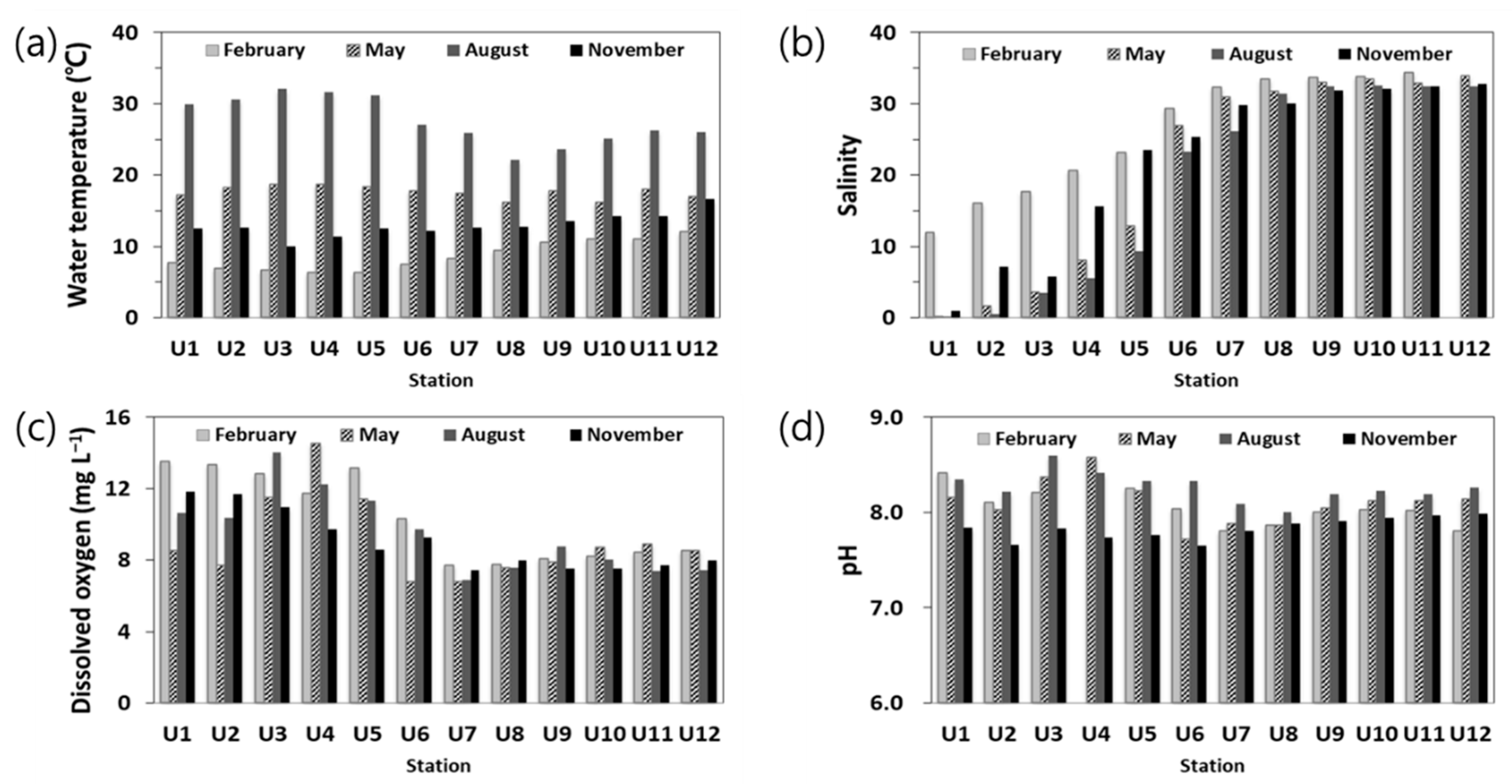
3.2.1. Temperature, Salinity, Dissolved Oxygen (DO), and pH

We surveyed the temperature, salinity, DO, and pH of the water body. The annual variation of water temperature was in the range of 6.32–32.13 °C (average: 15.13 °C) (Figure 3a). The water temperature changed according to the season (p < 0.01): lower temperatures were recorded in February during the winter season and higher temperatures were recorded during the summer season; seasonal water temperature changes are a typical characteristic of temperate latitudes. The water temperature differences between the surface and bottom waters were between 0–7.74 °C. These differences increased toward Ulsan Bay because the depth of the water increased, and higher values were recorded in the summer season compared to the winter season (p < 0.01).
Salinity changes in the surface water ranged between 0.15–34.37 (average: 33.95) (Figure 3b). Salinity values were relatively high (average: 23.61) in February (winter) and lower (average: 19.15) in August (summer). The salinity differences between surface and bottom waters were in the 0.00–14.39 range (average: 2.20). We spatially divided the data into two groups: the first group (U1–U5) had large salinity changes that exceeded 10; the second group (U6–U12) had smaller salinity changes, less than 5, depending on the season.
DO concentrations in surface water were in the range of 6.78–14.54 mg L−1 (average: 8.82 mg L−1) (Figure 3c). We also divided the data into two groups based on season (similar to the salinity groups): one group (U1–U6) had larger changes that exceeded 3 mg L−1 (range: 3.07–5.64 mg L−1); the other group (U7–U12) had relatively smaller changes less than 2 mg L−1 (range: 0.41–1.52 mg L−1), depending on the season. DO concentration differences between surface and bottom waters ranged between 0–8.54 mg L−1 (average: 1.46 mg L−1). Larger differences in the DO concentrations between the surface and bottom waters appeared at U2–U5 (except for the February survey).
pH changes in surface water ranged between 7.65–8.60 (average: 7.90) (Figure 3d); seasonal pH changes were relatively larger at U1–U6, similar to the DO concentrations (p < 0.01). Average pH values were relatively higher in August and lower in November.

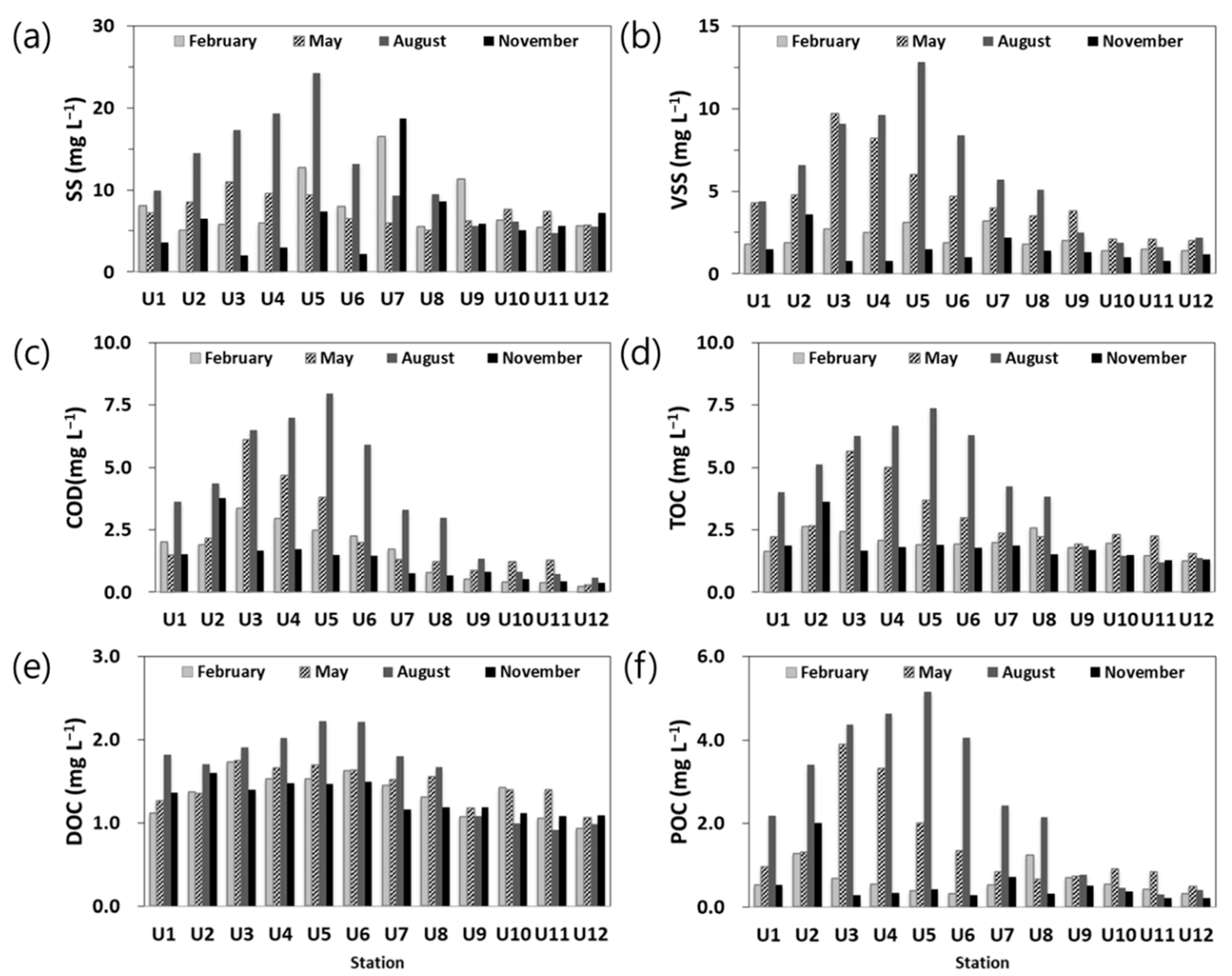
3.2.2. Organic Contents
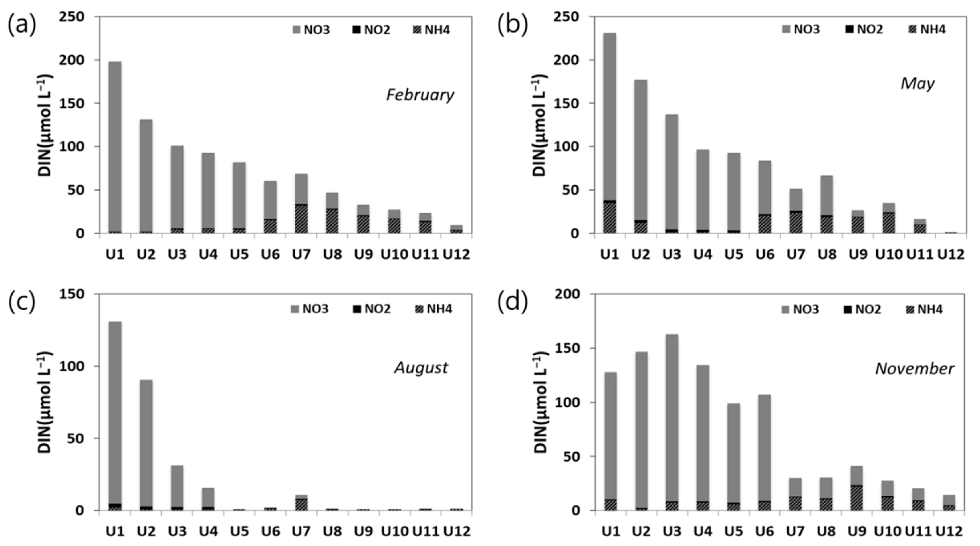
SS concentrations in the surface water were between 2.00–24.20 mg L−1 (average: 8.36 mg L−1), and SS concentrations in the bottom water (U9–U12) were between 5.20–45.00 mg L−1 (average: 10.91 mg L−1) (Figure 4a). These results showed relatively higher SS concentrations in August, similar to the results from another study [29] because precipitation is heavy in Korea during summer. We spatially divided the data into two groups for SS concentrations. The differences in SS concentrations between the surface and bottom waters were relatively high at U1–U7 and lower at U8–U12. It was found that the SS input into the upper estuary originated from small streams.
Total SS were divided into volatile suspended solids (VSS) and fixed suspended solids (FSS); in this study, we focused only on VSS. The changes in VSS concentrations in the surface water were between 0.80–12.80 mg L−1 (average: 3.49 mg L−1), and the VSS in the bottom water (U9–U12) ranged between 10.90–5.40 mg L−1 range (average: 2.11 mg L−1) (Figure 4b). High VSS contents in TSS indicate high amounts of organic matter in the water samples. Therefore, we calculated the VSS/TSS ratio, and the ratio showed relatively higher values, i.e., an average of 0.41 (range: 0.12–0.88), in the surface water, with lower values, i.e., an average of 0.22 (range: 0.12–0.38), in the bottom water. Seasonally, the VSS/TSS ratio showed a high value with an average of 0.59 (range: 0.28–0.88) in May, especially at U4 and U5, which displayed relatively high values, i.e., 0.88 and 0.85, respectively. Spatially, U2 and U3 (upper estuary) showed higher values than stations in the lower estuary except for the August survey. In August, the surface water of U6 and U7 showed a higher VSS/TSS ratio than other stations because of high amounts of VSS input to the Taehwa estuary through the Dong River during the summer, which is a season with high rainfall. The bottom water at U9 showed the highest SS value (45 mg L−1) in August, but VSS/TSS appeared to be low at 0.12, which indicated high amounts of inorganic matter in the water.
The changes in the COD concentration in the surface water ranged between 0.24–7.97 mg L−1 (average: 2.20 mg L−1). COD concentrations in the bottom water ranged between 0.23–1.52 mg L−1 (average: 0.66 mg L−1) (Figure 4c). COD concentrations showed a similar tendency to the VSS concentrations (r = 0.914, p < 0.01), but COD concentrations in August showed higher values on average, 3.76 mg L−1, compared to other months. Spatially, higher COD values appeared at U3 and U4 in most seasons, but the highest concentration of COD was observed at U5 in August.
TOC was the calculated sum of POC and DOC in this study. TOC concentration changes ranged between 1.21–7.37 mg L−1 (average: 2.71 mg L−1) in the surface water and 0.90–2.44 mg L−1 (average: 1.52 mg L−1) in the bottom water (Figure 4d). The highest concentration of TOC in the surface water was an average of 4.14 mg L−1 in August, similar to the COD concentrations. TOC was compared to the spatial distributions of VSS and COD concentrations. The TOC results in the upper estuary showed higher values except for some of the stations. There was a strong positive correlation between POC and DOC (r = 0.792, p < 0.01). Generally, DOC concentrations were higher than POC concentrations, but POC concentrations were higher in the upper estuary (U1–U6) in May and August (Figure 4e,f).
Although VSS, COD, and TOC have different analysis methods, these three indicators allow the measurement of the concentration of organic matter. The respective correlations between VSS and COD, between VSS and TOC, and between COD and TOC were r = 0.914 (p < 0.01), r = 0.950 (p < 0.01), and r = 0.952 (p < 0.01), i.e., strong positive correlations. VSS, COD, and TOC exhibited seasonal changes, i.e., higher concentrations in August and lower concentrations in February or November. Spatial distributions showed that concentrations of the three variables increased from U1 to U3 and decreased from U3 to U12 in May, but the concentrations increased from U1 to U5 and decreased from U5 to U12 in August. COD concentrations were higher at U2–U3 compared with other stations, unlike VSS and TOC, in February and November. There were no differences between surface and bottom waters in terms of the VSS, COD, and TOC concentrations at U9–U12.

3.2.3. Nutrients

Sufficient nutrients (N, P) and appropriate water temperature are needed in the water column for phytoplankton growth [30,31,32,33]. We analyzed five nutrients: ammonium (NH4+-N), nitrite (NO2-N), nitrate (NO3-N), phosphate (PO43−-P), and silicate (SiO2-Si). Dissolved inorganic nitrogen (DIN, the sum of ammonium, nitrite, and nitrate) concentrations in the surface water showed a tendency to decrease toward the lower estuary regardless of season (Figure 5). Higher nutrient concentrations in the upper estuary are due to the input of industrial sewage, agricultural and livestock farming sewage, and urban wastewater, [34]; on the other hand, relatively lower nutrient concentrations in the lower estuary are due to dilution by seawater [35,36]. Relatively low DIN concentrations of 23.89 μmol L−1 (range: 0.68–130.77 μmol L−1) were found in August (Figure 5c). High precipitation in summer (August) transported the nutrients to the open sea, so the nutrient concentration was low because nutrients have a short retention time in water [37]. Nitrate nitrogen generally accounted for a high proportion of DIN (Figure 5), i.e., 3.5–98.8% (average: 60.9%) of DIN. The nitrate ratios in DIN appeared to be relatively high in the upper estuary compared to the lower estuary. The nitrate ratio decreased and the ammonium ratio increased from U5 to U12 in August. The nitrate ratio of DIN was 92.1% (U1–U4: 84.1–96.9%) in the upper estuary and 9.5% (U5–U12: 3.5–22.3%) in the lower estuary. After the Dong River joined the Taehwa River, nitrate ratios decreased in all surveys.
Ammonium concentrations of the surface water ranged between 0.62–34.86 μmol L−1 (average 9.14 μmol L−1) (Figure 6a). Low ammonium concentrations (average: 1.50 μmol L−1) were found in August and high ammonium concentrations (average: 13.86 μmol L−1) were found in May. The highest ammonium concentration was found at U1 and the lowest ammonium concentrations were found at the U2–U5 stations in May. This is the result of a phytoplankton bloom, because phytoplankton take up ammonium ions first rather than other nitrogen forms [38,39]. There were no differences in nitrite concentrations among stations in February and November (Figure 6b). On the other hand, nitrite concentrations gradually decreased from the upper to lower estuary in May and August (except for U5 and U6). Nitrate concentrations also gradually decreased from the upper to lower estuary in all seasons (Figure 6c). Distributions of phosphate concentrations displayed a similar pattern to those for ammonium (r = 0.544, p < 0.01) (Figure 6d). Phosphate concentrations appeared to be relatively low in the upper estuary (U1–U5) and high in U7 (U6 in August) and then decreased toward the open sea. Seasonally, there was a lower concentration in August except for U6 and U7, and the highest concentration (0.514 μmol L−1) was measured at U6 in August. This meant that the water had a higher phosphate concentration when flowing into the estuary from the Dong River in summer. Silicate concentrations were higher (average: 1.57 μmol L−1) in November than in other months; spatially high values appeared in the upper estuary with low values in the lower estuary (Figure 6d).

3.2.4. Chl.a

Chl.a concentrations were in the 0.24–127.20 μg L−1 range (average: 8.68 μg L−1) in the surface water and were in the 0.29–2.31 μg L−1 range (average: 1.30 μg L−1) in the bottom water (Figure 6f). Seasonally, chl.a concentrations were low in February, in the 0.24–1.75 μg L−1 range (average: 0.57 ± 0.42 μg L−1). Chl.a concentrations were in the 0.46–38.22 μg L−1 range (average: 8.62 ± 12.72 μg L−1) in May, with higher values at U3 and U4 because of the algal bloom, i.e., 38.22 μg L−1 and 34.52 μg L−1, respectively. Chl.a concentrations were in the 0.64–23.14 μg L−1 range (average: 12.51 ± 7.81 μg L−1) in August. Chl.a concentrations were in the 0.95–127.20 μg L−1 range (average: 13.64 ± 34.34 μg L−1) in November and the highest value was 127.20 μg L−1 at U2. As mentioned in the Introduction, non-toxic algal blooms dominated by Cryptomonads occur in the upper estuary (U2–U4) during the dry seasons (November–May) in the Taehwa estuary [24,25,26]. We also observed an algal bloom in a small area in November; therefore, the chl.a concentrations were high in that area.

3.3. Phytoplankton

3.3.1. Species Composition

A total of 83 phytoplankton species were recorded in the Taehwa River estuary during the survey period. The most abundant group was Bacillariophyceae, with 49 species (58%, as a percentage of the total number of species), followed by Dinophyceae with 16 species (19%), Chlorophyceae with 11 species (13%), Euglenophyceae with 2 species (2%), Dictyochaceae with 2 species (2%), Cryptophyceae with 2 species (2%), and Cyanophyceae with 1 species (1%). Chaetoceros sp. (Bacillariophyceae) were the most abundant, i.e., five species, and four Protoperidinium sp. (Dinophyceae) were recorded. Bacillariophyceae appeared with a high emergence rate in this study area. Euglenophyceae and Chlorophyceae appeared in the upper estuary because these are freshwater plankton species, and Dinophyceae appeared in the lower estuary.
The most abundant taxa were Bacillariophyceae, with 32 species in February, and Dinophyceae, with 11 species in August. Seasonally, 41 phytoplankton species emerged in February. Bacillariophyceae had a high rate of emergence, with 32 species (78%), and Dinophyceae with 3 species (7.3%). Euglenophyceae emerged with two species (4.9%), and Dictyochaceae, Cryptophyceae, Chlorophyceae, and Cyanophyceae emerged with one species (2.4%) each (Figure 7a). A total of 28 species emerged in August; the most abundant taxa were Bacillariophyceae with 23 species (82.1%), Chlorophyceae with 3 species (10.7%), and Dinophyceae and Dictyochaceae with 1 species (3.6%) each (Figure 7b). The number of species were higher in August (52 species in total) than in the other seasons. Among the emergent species, there were 29 Bacillariophyceae species (55.8%), 11 Dinophyceae species (21.2%), 9 Chlorophyceae species (17.3%), 2 Dictyochaceae species (3.85%), and 1 Euglenophyceae species (1.92%) (Figure 7c). In November, a total of 34 species emerged, and there were 20 Bacillariophyceae species (58.8%), 8 Dinophyceae species (2.5%), 3 Chlorophyceae species (8.8%), 2 Dictyochaceae species (5.9%), and 1 Euglenophyceae species (2.9%) (Figure 7d).

3.3.2. Phytoplankton Population and Dominant Species

The monthly average phytoplankton population ranged between 87–375 cells mL−1 in this study. The phytoplankton population was relatively low in May and high in August. Spatially, there was a higher population in the upper estuary than in the lower estuary. (Figure 8a). These results, compared to other studies, showed that the average phytoplankton population in the Taehwa estuary was higher than that in the Seomjin River estuary, which was in the 137–212 cells mL−1 range [40], lower than that in Ulsan Bay, which was in the 486–10,456 cells mL−1 range during summer [41], and lower than that in the Nakdong River, which was in the 642–6064 cells mL−1 range [42].
The average phytoplankton population was 100 cells mL−1 in February, with the highest value of 444 cells mL−1 found at U1 and U2 (Figure 8a). Bacillariophyceae accounted for 51.0% of the total population (Figure 8b). Spatially, Fragilaria construens dominated at U1, and Euglena spp. dominated at U4–U6. The average phytoplankton population was 87 cells mL−1 in May, with the highest value of 456 cells mL−1 at U4 (Figure 8a). Unidentified small-sized flagellates were extremely dominant, i.e., 88–96% at U3–U5 (Figure 8b). The highest average population was measured in August, i.e., 375 cells mL−1 (Figure 8a). Diatoms mostly dominated at all stations, and the Cyclotella spp. population among diatoms was high in the upper estuary, and Chaetoceros spp. were abundant in the lower estuary. These results are similar to those of a previous study [43] in which Chaetoceros compressus dominated in the Taehwa River estuary during summer. More diatoms (Chaetoceros spp., Skeletonema spp.) occurred at U7–U8, because high amounts of nutrients were provided from the Dong River due to high summer precipitation. Actinastrum hantzschii var. fluviatile dominated at U1, and unidentified flagellates dominated at U5–U6. The average phytoplankton population in November was 139 cells mL−1. The highest value of 1322 cells mL−1 was measured at U2, and relatively low values were found in the 1.2–176.4 cells mL−1 range at other stations (Figure 8a). Cryptomonas spp. dominated at most stations (Figure 8b) in this study; these results are similar to a previous study [25] in which Cryptomonas sp. dominated near U3 in December 2010 (winter season). Silicate concentrations in the water body were higher in November than in other months (Figure 6d) because Cryptomonas sp. dominated in November. Diatoms take up silicate for their cells unlike other phytoplankton, so the higher silicate concentrations in November allowed Cryptomonas sp. to become dominant in the water. Cryptomonas sp. can live in both freshwater and seawater, and if the population increases rapidly (blooms), the water color can turn brown and cause bad odors (e.g., a fishy smell).

4. Discussion

4.1. Seasonal Environmental Factors According to Water Flow

The Nakdong River flood control office provides hydrological data for the Taehwa River estuary, and this observation point is located between U3 and U4 (www.nakdongriver.go.kr). These hydrological data are shown in Table 1, with average values of the monthly water level and the rate of flow. According to the Korean Meteorological Administration data (www.kma.go.kr), the total precipitation of Ulsan city was 12 mm in February 2012, which is in the dry season. The average water level was 0.96 m, and the average flow rate was 6.10 m3 s−1, which are lower values than those in other seasons. High salinity values were recorded in the upper estuary, which was affected by the seawater due to the lower precipitation during the dry season (February). Algal blooms in the Taehwa River estuary occur under low water levels [24]. In this study, we did not detect an algal bloom in February, which was during the dry season, because the water level was higher and the flow rate was double compared to the results of the other study [24]; we also found that other factors disrupt algal blooms. The average flow rates were 11.33 m3 s−1 in May and 12.50 m3 s−1 in August, which are higher than the values of the other seasons due to high precipitation (Table 1). Typically, there is high rainfall in summer (August) in Korea, which was also experienced during this study. High amounts of inorganic and organic matter from land are supplied to the Taehwa River and higher SS concentrations were found at the upper estuary (U1–U5) where there are relatively low current velocities in May and August. As a result, phytoplankton grew better in a low current environment in May than in August because precipitation was lower and nutrients were abundant; these nutrients were provided from upper sections of the river, and the phytoplankton had enough time to take up the nutrients and grow.

4.2. Water Retention Time and Algal Blooms

We measured the water retention time using two floated buoys for each survey in the Taehwa estuary (upper: March 2012; lower: November 2012). The water in the upper estuary had a long retention time and moved a short distance. On the other hand, the water in the lower estuary had a short retention time except for the stagnation zone (caused by eddy currents), and U2–U3 had a long retention time (Figure 2a, A–B section). As a result, if nutrients were provided to U2–U3 from a small stream, the possibility of algal bloom occurrence would increase as the phytoplankton would have enough time to grow. Algal blooms could also extend to U3–U4, which also had a relatively long retention time. Many studies [24,25,26] have investigated the occurrence of algal blooms near U2–U3, similar to our study. Unlike the upper estuary, in the lower estuary, the possibility of algal bloom occurrence was low even though nutrients were provided from the Dong River because the water flows fast toward the open sea and is diluted by the seawater.

4.3. Water Quality Assessment

Water quality is commonly found to be poor near ports, bays, and estuaries because of the many land-based pollutants flowing into the water. In the ROK, there is a river water environmental standard concerning water quality and water ecosystems in the official environmental policy. According to this standard, water quality is divided into seven grades: very good (Ia), good (Ib), slightly good (II), normal (III), slightly poor (IV), poor (V), and very poor (VI). Water quality in the Taehwa River was considered very poor (VI) in 1997 because of the growth of cities and industrial developments; however, the water quality and ecosystem recovered and were re-graded to be good (Ib) after the Ulsan local government actively implemented the environmental renewal project to improve the Taehwa River water quality. The 2012 water quality in the Taehwa River estuary was estimated based on the results in this study. There are eight total indicators for the river water environmental standard: pH, BOD (biochemical oxygen demand), COD, TOC, SS, DO, TP, and coliform groups (total coliform, fecal coliform). In this study, we investigated six indicators (BOD and the coliform group were not included). The water quality grade was individually calculated for each survey and all stations were graded good (Ib) or slightly good (II) in February. A good (Ib) grade was calculated for U1 and U2, and a slightly poor (IV) grade was calculated for U3 because of higher COD and TOC concentrations. In May, a normal (III) grade was given to U4 and U6, a good (Ia) grade was given to U12, and a slightly good (II) grade was given to the other stations. In August, lower water quality grades were calculated as slightly poor (IV) for U2 and bad (V) for U3–U6 because of higher COD and TOC concentrations. The other stations were considered good (Ib) or normal (III) in August. In November, good (Ib) or slightly good (II) grades were obtained, which indicates a better water environment compared to other surveys. As a result, we argue that in the upper estuary, organic matter in the water in spring and summer needs to be managed to improve the water quality.
In the case of the estuary area, the water quality could also be calculated by the Marine Environment Standard [44], which is determined by the Ministry of Maritime Affairs and Fisheries (MOF). This marine environment standard has five grades: very good (I), good (II), normal (III), poor (IV), and very poor (V). The MOF evaluates seawater quality based on marine environmental standards through the national marine environmental monitoring system to grade the seawater of each region. The upper Taehwa River estuary (U6–U12) did not achieve the target grade twice in five years from 2013 to 2017 [45]; therefore, the Taehwa River estuary needs long-term continued management to improve water quality and to decrease the occurrence of algal blooms.

4.4. Chl.a and Biomass

The correlation coefficient was low between Chl.a and phytoplankton biomass in this study (R2 = 0.3451, linear regression). Seasonally, the correlation between Chl.a and phytoplankton biomass was high in February and November, but there was no correlation in August. These results are similar to those from a previous study [29], where the correlation between Chl.a and phytoplankton biomass was low because of small-sized diatoms in summer. This low correlation occurred because dominant species are different each season, and species have different characteristics such as their chl.a concentrations per cell, cell size, etc. [43,46,47,48]. Chl.a concentrations are determined based on the cell density of flagellates [46]. In this study, unidentified flagellates were dominant in May, but diatoms were dominant (>55%) in August. Therefore, our Chl.a data were underestimated in August when diatoms were dominant. Moreover, in the case of dominant nano–pico-sized phytoplankton, cell density could be underestimated because small-sized phytoplankton cannot be observed through a microscope [43,49,50,51,52]. Micro (20–200 μm)-sized phytoplankton grow well in a nutrient-rich environment, but pico (0.2–2 μm) and nano (2–20 μm)-sized phytoplankton grow at a high rate in a nutrient-poor environment [50,53]. Ammonium and phosphate had low concentrations at U3–U5 in May, and chl.a concentrations were high but biomasses were low, which meant that there were numerous nano–pico-sized flagellates at U3–U5 in May. Similarly, a prior case study documented that numerous pico- and nano-sized phytoplankton appeared in Ulsan Bay during a summer before the rains [54].

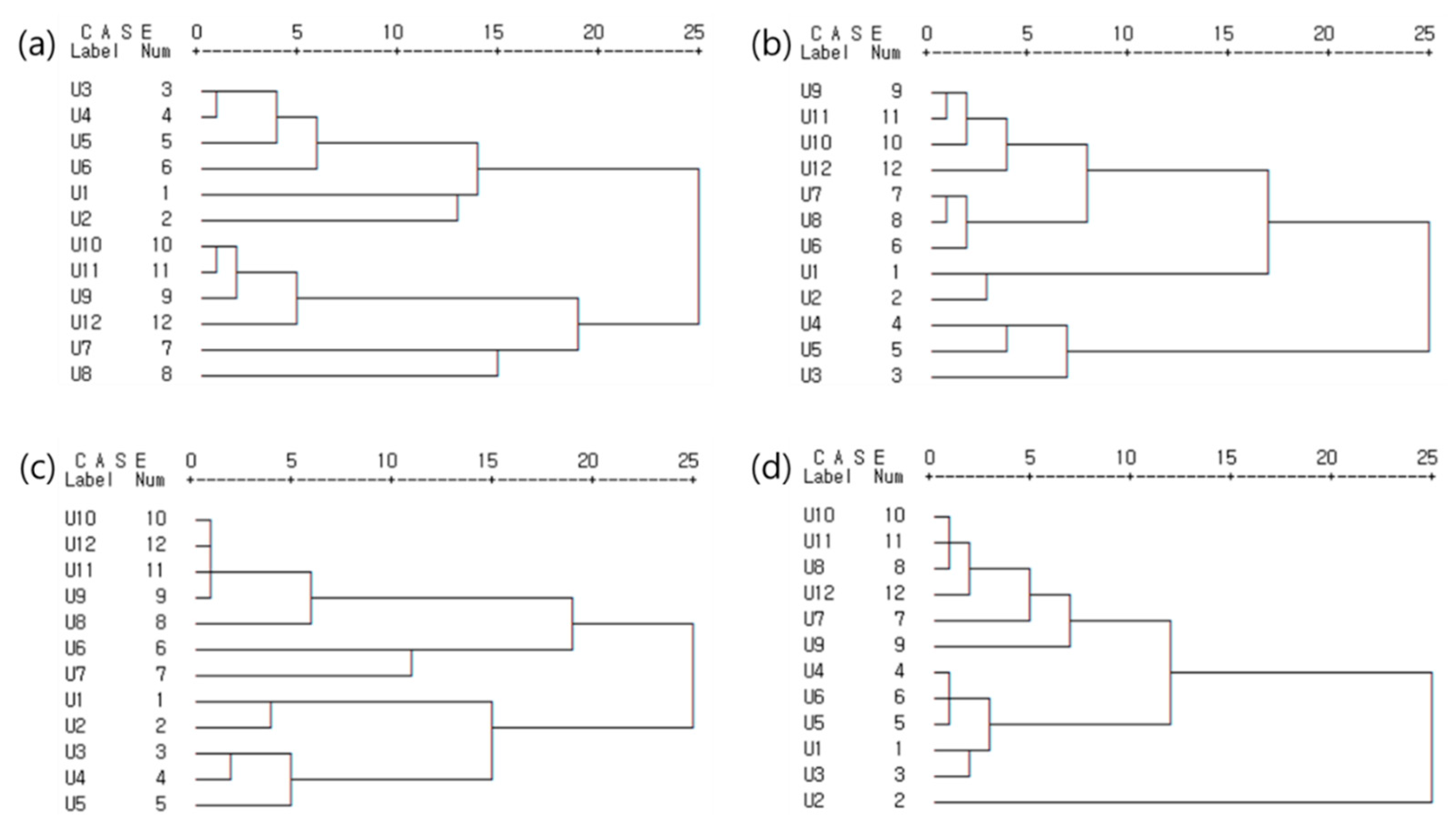
4.5. Estuary Classification

This estuary was physically divided into several groups through clustering analysis. First, two or three groups were created based on water quality factors. In February, the estuary was divided into two groups, U1–U6 and U7–U12 (Figure 9a). In May, the estuary was divided into three groups (U1–U2, U3–U5, and U6–12) because an algal bloom occurred in the U3–U5 section (Figure 9b). In August, the estuary was divided based on the Dong River connection, i.e., into the U1–U5 group and U6–U12 group (Figure 9c). In November, the estuary was divided into two groups, U1–U6 and U7–U12, except for U2 where an algal bloom occurred, which is similar to the result obtained for February (Figure 9d). In summary, the Taehwa River estuary was divided into two groups based on the area between U5 and U6 (spring and summer) and between U6 and U7 (fall and winter).
The Taehwa River estuary was also divided into two groups based on phytoplankton species composition. One group was the upper estuary (U1–U6) where freshwater phytoplankton occurred, such as Actinastrum hantzschii var. fluviatile, Cryptomonas spp., Cyclotella spp., and Scenedesmus spp., and the other group was the lower estuary (U7–U12), where seawater phytoplankton occurred, such as Chaetoceros spp., Leptocylindrus danicus, Prorocentrum triestinum, Protoperidinium spp., and Skeletonema spp. (Figure 10). As a result, the Taehwa River estuary was divided into the upper estuary, i.e., U1–U6, and the lower estuary, i.e., U7–U12; this division was also made in a previous study [27], which classified the estuary based on sedimentary environmental factors. Based on the results obtained pertaining to the water quality, sediment environmental factors, and biological data, the Taehwa River estuary can be spatially divided into two areas: U1–U6 and U7–U12.

4.6. Causes of Seasonal Algal Blooms

At most stations, chl.a concentrations were low in February (Figure 11a) and phytoplankton cell densities were also low except at some stations. Because the water temperature and nutrient concentrations were low at the starting point of the algal bloom in February, both temperature and nutrients were found to be important factors in the growth of phytoplankton. If N < 1 μmol L−1, P < 0.2 μmol L−1, or S < 2 μmol L−1 in the water column, phytoplankton growth is limited [55]. Average phosphate concentrations were 0.125 μmol L−1, i.e., lower values than the nutrient limitation at U1–U5 (where algal blooms frequently occurred during other seasons). Therefore, the chl.a concentration and phytoplankton population were low in February. Euglena spp., a pollution indicator species, were dominant at U4–U6, especially at U5. Euglena spp. are freshwater species that occur in stagnant waters of urban rivers, most of which are polluted in ROK [56,57]. Euglena spp. are sensitive to nutrients and cause large algal blooms when nutrients are supplied and water temperature increases in spring [58,59]; therefore, if nutrients are supplied to the upper estuary during the dry winter season, a green tide could occur due to Euglena spp. growth. Water temperatures are increasing in the winter because of climate change, so the possibility of winter algal blooms could also increase after precipitation in the Taehwa River estuary.
Chl.a concentrations were high at U3–U5 where an algal bloom started in May in this study (Figure 11b). The phytoplankton population was also high at U3–U5 and the dominant species were unidentified flagellates (88–96%). Because the size of unidentified flagellates was less than 20 μm, we did not distinguish between species. We found that at the beginning of the algal bloom in May, nano–pico-sized flagellates dominated in the survey area. The growth of flagellates increased significantly as nutrients were supplied, so ammonium and phosphate concentrations were low at U3–U5 in May (Figure 11b). Additionally, another study concluded that nano–pico-sized plankton absorbed more phosphate than other sized plankton [60], which is in agreement with the results of our study.
In August, A. hantzschii var. fluviatil Cyclotella sp., which is a freshwater species, dominated the upper estuary. Similar to the survey results of May, many Cyclotella sp. and nano–pico-sized flagellates appeared at U2–U5, which resulted in high chl.a concentrations and a low phytoplankton population (Figure 11c). Chaetoceros sp. and Skeletonema sp., which are seawater species, dominated at U7–U8, contrary to the findings for the upper estuary. It was found that organic matter and nutrients (especially phosphate) were supplied from the Dong River. The abundance of dominant dinoflagellates increased during summer to fall from the lower estuary of the Taehwa River to the coastal area of Ulsan Bay [43]. More Dinophyceae appeared in August and November than in other seasons at U9–U12. Although the number of diverse species increased, the Dinophyceae population decreased to 0.7–13.3% at U9–U12, except for U8 (39.5%). Algae flourish where the water temperature is 25°C and salinity is 30–35 [61], so water temperature and salinity appear to be good conditions for algal growth during summer at U9–U10; however, Chaetoceros sp. and Skeletonema sp. were dominant and both algae are rival species to red tide species, so an algal bloom did not occur at U9–U10 during summer. Another study showed that Chaetoceros sp. dominated near U8 in summer [43].
In November, a Cryptomonas sp. bloom occurred at U2; it is known that Cryptomonas sp. blooms every winter. Cryptomonas spp. cause toxic Karlodinium veneficum blooms in a well-nourished environment [62]. Fortunately, K. veneficum was not discovered during survey periods, but we still conclude that attention should be paid to toxic blooms. High amounts of Fe and P in water bodies accelerate the growth of Cryptomonas sp. and cause blooms of this species [63]. There were higher trace metal concentrations that exceeded the ERL (effect range low) standard in the surface sediment of U2 compared to the other stations, and trace metals Fe, Cu, As, and Zn showed higher values [27]. Materials could be exchanged between the water and sediment, with more Fe and P in sediment released into the water column [63]. High levels of nutrients, including phosphate concentrations, were found at U1–U2 (Figure 11d). As a result, high Fe and P accelerated the Cryptomonas sp. bloom in November, and the long water retention time allowed phytoplankton to absorb sufficient nutrients. Another study has shown that algal blooms occurred when the river flow rate was slow because of low precipitation in the Hyeonsang River estuary [64].
To summarize, this section details the seasonal causes of algal blooms considering various water and environmental parameters. Algal blooms in the Taehwa River estuary broke out at U2 and spread toward the lower estuary; the main causes of the algal blooms were nutrient concentrations and water retention time. In this study, we observed two algal bloom phenomena: one was unidentified flagellate blooms, which consisted of nano–pico-sized phytoplankton in May, and the other was a Cryptophyceae bloom in November 2012. We did not observe any algal blooms in August and February because the retention time of nutrients in the water was short in summer because of greater river flow, and in winter, nutrients were limited because of low precipitation. Further investigations are required to determine the effect of land-based pollutants, including nutrients and organic matter, on the river water quality through the streams or rivers that join the Taehwa River. The phytoplankton community and algal bloom surveys according to various scales of precipitation will be investigated in a further study.

5. Conclusions

The ecology in the Taehwa River estuary of ROK has recovered through environmental improvement projects; however, algal blooms still occur in the upper estuary from winter to spring, especially in the dry season. In this study, we investigated the seasonal cause of algal blooms based on various water environmental factors. We also surveyed the seasonal changes in the phytoplankton community as well as water flow characteristics using floating buoys. The main cause of phytoplankton growth was the supply of nutrients from water supplied from a connecting river and the long water retention time. Algal blooms did not occur in February 2012 because of P limitation, even though this period was relatively dry and the total precipitation was at its lowest (12 mm for the month). On the other hand, algal blooms of nano–pico-sized flagellates occurred, which increased rapidly at U3–U4 in May. The water flow rate increased because of higher precipitation in August, resulting in a shorter water retention time; for these reasons, algal blooms did not occur in August. Under these circumstances, the phytoplankton in freshwater dominated in the upper estuary, but Chaetoceros sp. and Skeletonema sp., which compete with red tide algae, were dominant in the lower estuary after nutrients were introduced from the Dong River. An algal bloom of non-toxic Cryptophyceae occurred at U2 in November because of the nutrients and long water retention time. We divided the Taehwa River estuary based on cluster analysis and distinguished the predominantly freshwater areas from the predominantly seawater areas. Our results indicate that a management strategy that focuses on reducing the supply of nutrients (N, P) into the estuary is needed to reduce the occurrence of algal blooms. Further investigations are needed to generalize the effects of land-based pollutant inflow into the Taehwa River estuary on algal bloom generation, which should include more streams with different environmental characteristics, data on water quality with different magnitudes, and exposure periods.

Author Contributions

Conceptualization, B.-R.S., H.-C.K. and C.-S.K.; methodology, B.-R.S., J.-H.K., K.-W.P. and W.-A.L.; formal analysis, C.-S.K., J.-H.K., K.-W.P. and W.-A.L.; investigation, H.-C.K., C.-S.K. and J.-H.K.; validation, B.-R.S., C.-S.K., J.-H.K. and W.-A.L.; visualization, B.-R.S. and K.-W.P.; writing—original draft, B.-R.S.; writing—review and editing, B.-R.S., H.-C.K. and W.-A.L.; project administration, W.-C.L.; funding acquisition, W.-C.L. All authors have read and agreed to the published version of the manuscript.

Funding

This research was funded by the National Institute of Fisheries Science, Republic of Korea (Grant No. R2020050).

Acknowledgments

The authors would like to thank our colleagues for their assistance with sampling and analyses. The authors also thank the reviewers for their useful comments and suggestions to improve the scientific quality of the manuscript.

Conflicts of Interest

The authors declare no conflict of interest.

References

  1. Hallegraeff, G.M. Harmful algal blooms in the Australian region. Mar. Pollut. Bull. 1992, 25, 186–790. [Google Scholar] [CrossRef]
  2. Tang, D.; Kester, D.R.; Ni, I.-H.; Qi, Y.; Kawamura, H. In situ and satellite observations of a harmful algal bloom and water condition at the Pearl River estuary in late autumn 1998. Harmful Algae 2003, 2, 89–99. [Google Scholar] [CrossRef]
  3. Anderson, D.M.; Burkholder, J.M.; Cochlan, W.P.; Gilbert, P.M.; Gobler, C.J.; Heil, C.A.; Kudela, R.; Parsons, M.L.; Rensel, J.E.J.; Townsend, D.W.; et al. Harmful algal blooms and eutrophications: Examining linkages from selected coastal regions of the United States. Harmful Algae 2008, 8, 39–53. [Google Scholar] [CrossRef] [PubMed] [Green Version]
  4. Paerl, H.W. Assessing and managing nutrient-enhanced eutrophication in estuarine and coastal waters: Interactive effects of human and climatic perturbations. Ecol. Eng. 2006, 26, 40–54. [Google Scholar] [CrossRef]
  5. Howarth, R.W.; Bilen, G.; Swaney, D.; Townsend, A.; Jaworski, N.; Lajtha, K.; Oowning, J.A.; Elmgren, R.; Caraco, N.; Jordan, T.; et al. Regional nitrogen budgets and riverine N and P fluxes for the drainages to the North Atlantic Ocean: Natural and human influences. Biogeochemistry 1996, 35, 75–79. [Google Scholar] [CrossRef]
  6. D’Elia, C.F. Too much of a good thing: Nutrient enrichment of the Chesapeake Bay. Environment 1987, 29, 2. [Google Scholar] [CrossRef]
  7. National Research Council (NRC). Clean Coastal Waters: Understanding and Reducing the Effects of Nutrient Pollution; National Academy Press: Washington, DC, USA, 2000. [Google Scholar]
  8. Clesceri, E.J. Sources and Depositional Patterns of Particulate Organic Matter in the Neuse River Estuary, North Carolina (USA). Ph.D. Thesis, University of North Carolina at Chapel Hill, Chapel Hill, NC, USA, February 2004. [Google Scholar]
  9. Moore, S.K.; Trainer, V.L.; Mantua, N.J.; Parker, M.S.; Laws, E.A.; Backer, L.C.; Fleming, L.E. Impacts of climate variability and future climate change on harmful algal blooms and human health. Environ. Health 2008, 7, S4. [Google Scholar] [CrossRef] [Green Version]
  10. Rabalais, N.N.; Turner, R.E.; Diaz, R.J.; Justic, D. Global change and eutrophication of coastal waters. ICES J. Mar. Sci. 2009, 66, 1528–1537. [Google Scholar] [CrossRef]
  11. Cloern, J.E.; Schraga, T.S.; Lopez, C.B.; Knowles, N. Climate anomalies generate an exceptional dinoflagellate bloom in San Francisco Bay. Geophys. Res. Lett. 2005, 32, L14608. [Google Scholar] [CrossRef] [Green Version]
  12. Jahan, R.; Choi, J.K. Climate regime shift and phytoplankton phenology in a macrotidal estuary: Long-term surveys in Gyeonggi Bay, Korea. Estuaries Coasts 2014, 37, 1169–1187. [Google Scholar] [CrossRef]
  13. Revstock, G.A.; Kang, Y.S. A comparison of three marine ecosystems surrounding the Korean peninsula: Responses to climate change. Prog. Oceanogr. 2003, 59, 357–379. [Google Scholar] [CrossRef]
  14. Kim, S.; Zhang, C.-I.; Kim, J.-Y.; Oh, J.-H.; Kang, S.; Lee, J.B. Climate variability and its effects on major fisheries in Korea. Ocean Sci. J. 2007, 42, 179–192. [Google Scholar] [CrossRef]
  15. Lee, M.O.; Kim, J.K. Characteristics of algal blooms in the southern coastal waters of Korea. Mar. Environ. Res. 2008, 65, 128–147. [Google Scholar] [CrossRef]
  16. Lee, M.O.; Kim, B.K.; Kwon, Y.; Kim, J.K. Characteristics of the marine environment and algal blooms in Gamak Bay. Fish. Sci. 2009, 75, 410–411. [Google Scholar] [CrossRef]
  17. Shim, J.M.; Hwang, J.D.; Jeong, C.S.; Lee, Y.H.; Jeon, K.A.; Kwong, K.Y. The influence of oceanic conditions on the occurrence of Cochlodinium polykrikoides blooms in the East Sea. J. Environ. Sci. 2010, 19, 1385–1395. [Google Scholar] [CrossRef]
  18. Lee, J.; Han, M.-S. Change of blooming pattern and population dynamics of phytoplankton in Masan Bay, Korea. J. Korean Soc. Oceanogr. 2007, 12, 147–158. [Google Scholar]
  19. Kim, H.G.; Jung, C.S.; Lim, W.A.; Lee, C.K.; Kim, S.Y.; Youn, S.H.; Cho, Y.C.; Lee, S.G. The spatio-temporal progress of Cochlodinium polykrikoides blooms in the coastal waters of Korea. Korean Soc. Fish. Aquat. Sci. 2001, 34, 691–696. [Google Scholar]
  20. Khim, J.S.; Lee, K.T.; Kannan, K.; Villeneuve, D.L.; Giesy, J.P.; Koh, C.H. Trace organic contaminants in sediment and water from Ulsan Bay and its vicinity, Korea. Arch. Environ. Contam. Toxicol. 2001, 40, 141–150. [Google Scholar]
  21. Koh, C.H.; Kim, G.B.; Maruya, K.A.; Anderson, J.W.; Jones, J.M.; Kang, S.G. Induction of the P450 reporter gene system bioassay by polycyclic aromatic hydrocarbons in Ulsan Bay (South Korea). Environ. Pollut. 2001, 111, 437–445. [Google Scholar] [CrossRef]
  22. Ra, K.; Kim, J.K.; Hong, S.H.; Yim, U.H.; Shim, W.J.; Lee, S.Y.; Kim, T.O.; Lim, J.; Kim, E.S.; Kim, K.T. Assessment of pollution and ecological risk of heavy metals in the surface sediments of Ulsan Bay, Korea. Ocean Sci. J. 2014, 49, 279–289. [Google Scholar] [CrossRef]
  23. Ulsan City. Ulsan Environment Report; Ulsan City Hall: Ulsan, Korea, 2008; Available online: http://www.ulsan.go.kr/rep/ghpaper4 (accessed on 6 April 2020).
  24. Cho, H.-J.; Yoon, Y.-B.; Kang, H.-S.; Yoon, S.-K. Characteristics of red tide blooms in the lower reaches of Taehwa River. J. Korean Soc. Water Wastewater 2011, 25, 453–462. [Google Scholar] [CrossRef]
  25. Sohn, E.R.; Park, J.I.; Lee, B.R.; Lee, J.W.; Kim, J.S. Seasonal variation of physic-chemical factors and size-fractionated phytoplankton biomass at Ulsan seaport of East Sea in Korea. Korean J. Microbiol. 2013, 49, 30–37. [Google Scholar] [CrossRef] [Green Version]
  26. Shin, M.K. Final Report: Research on Algal Bloom in the Taewha River; Ulsan Regional Environmental Technology Development Center: Ulsan, Korea, 2007. [Google Scholar]
  27. Sim, B.-R.; Kim, H.C.; Kim, C.-S.; Hwang, D.-W.; Park, J.-H.; Cho, Y.-S.; Hong, S.; Lee, W.-C. Spatio-temporal changes of sediment environment in the Taehwa River estuary, Ulsan of Korea. J. Coast. Res. 2018, 85, 41–45. [Google Scholar] [CrossRef]
  28. MLTMA (Ministry of Land, Transport and Maritime Affairs). Processes of the Korean Standard Methods for Marine Environment; MLTMA: Gwacheon-si, Korea, 2010; p. 493. (In Korean) [Google Scholar]
  29. Jung, S.W.; Lim, D.I.; Shin, H.H.; Jeong, D.H.; Roh, Y.H. Relationship between physic-chemical factors and chlorophyll-a concentration in surface water of Masan Bay: Bi-daily monitoring data. Korean J. Environ. Biol. 2011, 29, 98–106. [Google Scholar]
  30. Hecky, R.E.; Kilham, P. Nutrient limitation of phytoplankton in freshwater and marine environments: A review of recent evidence on the effect of enrichment. Limnol. Oceanogr 1998, 33, 796–822. [Google Scholar] [CrossRef] [Green Version]
  31. Del-Amo, Y.; Pape, O.L.; Treguer, P.; Quequuiner, B.; Menesquen, A.; Aminit, A. Impacts of high nitrate freshwater inputs on macrotidal ecosystems. I. Seasonal evolution of nutrient limitation for the diatom dominated phytoplankton of Bay of Brest (France). Mar. Ecol. Prog. Ser. 1997, 161, 213–224. [Google Scholar] [CrossRef]
  32. Twomey, L.; Thompson, P. Nutrient limitation of phytoplankton in seasonally open bar-built estuary: Wilson inlet, Western Australia. J. Phycol. 2001, 37, 16–29. [Google Scholar] [CrossRef]
  33. Hashimoto, T.; Nakano, S. Effect of nutrient limitation on abundance and growth of phytoplankton in a Japanese Pearl farm. Mar. Ecol. Prog. Ser. 2003, 258, 43–50. [Google Scholar] [CrossRef] [Green Version]
  34. Shen, Z.L.; Liu, Q. Nutrients in the Changjiang River. Environ. Monit. Assess. 2009, 153, 27–44. [Google Scholar] [CrossRef]
  35. Liu, S.M.; Hong, G.H.; Zhang, J.; Ye, X.W.; Jiang, X.L. Nutrient budgets for large Chinese estuaries. Biogeosciences 2009, 6, 2245–2263. [Google Scholar] [CrossRef] [Green Version]
  36. Chang, W.K.; Ryt, J.; Yi, Y.; Lee, W.C.; Kang, D.; Lee, C.H.; Hong, S.; Nam, J.; Khim, J.S. Improved water quality in response to pollution control measures at Masan Bay, Korea. Mar. Pollut. Bull. 2012, 64, 427–435. [Google Scholar] [CrossRef] [PubMed]
  37. Royer, T.V.; Tank, J.L.; David, M.B. Transport and fate of nitrate in headwater agricultural streams in Illinois. J. Environ. Qual. 2004, 33, 1296–1304. [Google Scholar] [CrossRef] [PubMed]
  38. Rendell, A.R.; Horrobin, T.M.; Jickells, T.D.; Edmunds, H.M.; Brown, J.; Malcolm, S.J. Nutrient cycling in the Great Ouse estuary and its impact on nutrient fluxes to the Wash, England. Estuar. Coast. Shelf Sci. 1997, 45, 653–668. [Google Scholar] [CrossRef]
  39. Hu, J.; Li, S. Modeling the mass fluxes and transformations of nutrients in the Pearl River Delta, China. J. Mar. Syst. 2009, 78, 146–167. [Google Scholar] [CrossRef]
  40. Kwon, K.Y. Behavior of Basic Ecological Components Along the Salinity Gradients in Low Turbidity Estuarine Water. Ph.D. Thesis, Pukyong National University, Busan, Korea, 2002. [Google Scholar]
  41. Lee, J.Y. Consideration of Environmental Factors on Phytoplankton and Dinoflagellate Cyst Distribution of Ulsan Bay in Summer. Master’s Thesis, Pukyong National University, Busan, Korea, 2007. [Google Scholar]
  42. Moon, C.H.; Choi, H.J. Studies on the environmental characteristics and phytoplankton community in the Nakdong River estuary. J. Korean Soc. Oceanogr. 1991, 26, 144–154. [Google Scholar]
  43. Yoon, Y.H.; Jeong, D.S. Spatio-temporal distributions of phytoplankton community and it’s variation characteristics in the Ulsan coastal waters. Southern east sea of Korea. J. Korean Soc. Mar. Environ. Energy 2019, 22, 159–171. [Google Scholar] [CrossRef]
  44. Ministry of Oceans and Fisheries (MOF). Marine Environment Standards; MOF: Sejong, Korea, 2018. [Google Scholar]
  45. Park, M.-O.; Lee, Y.-W.; Park, J.-K.; Kang, C.-S.; Kim, S.-G.; Kim, S.-S.; Lee, S.M. Evaluation of the seawater quality in the coastal area of Korea in 2013–2017. J. Korean Soc. Mar. Environ. Energy 2019, 22, 47–56. [Google Scholar] [CrossRef]
  46. Honjo, T.; Shimouse, T.; Hanaika, T.A. Red tide occurred at the Hakozaki fishing port, Hakada Bay, in 1973-The growth process and the chlorophyll content. Bull. Plankton Soc. Jpn. 1978, 25, 7–21. [Google Scholar]
  47. Curl, H.J.; McLeod, G.C. The physiological ecology of a marine diatom, Skeletonema costutum (Grev.) Cleve. J. Mar. Res. 1961, 19, 70–88. [Google Scholar]
  48. Türkoglu, M. Temporal variations of surface phytoplankton, nutrients and chlorophyll a in the Dardanelles (Turkish Straits system): A coastal station sample in weekly time intervals. Turk. J. Biol. 2010, 34, 319–333. [Google Scholar]
  49. Yoon, Y.H.; Rho, H.G.; Kim, Y.K. Seasonal succession of phytoplankton population in the Hamdok port, Northern Cheju Island. Bull. Mar. Cheju Natl. Univ. 1992, 16, 27–42. [Google Scholar]
  50. Maita, Y.; Odate, T. Seasonal change in size-fractionated primary production and nutrient concentrations in the temperate neritic water of Funka Bay, Japan. J. Oceanogr. Soc. Jpn. 1988, 44, 268–279. [Google Scholar] [CrossRef]
  51. Yoon, Y.H. Marine Environment and Phytoplankton Community in the Southwestern Sea of Korea; Choi, J.K., Ed.; The Plankton Ecology of Korean Coastal Waters, Donghwa Tech. Publ. Co.: Seoul, Korea, 2011; pp. 68–93. [Google Scholar]
  52. Guo, C.; Liu, H.; Zheng, L.; Song, S.; Chen, B.; Huang, B. Seasonal and spatial patterns of picophytoplankton growth, grazing and distribution in the East China Sea. Biogeosciences 2014, 11, 1847–1862. [Google Scholar] [CrossRef] [Green Version]
  53. Iriate, A.; Purdie, D.A. Size distribution of chlorophyll-a biomass and primary production in a temperate estuary (Southampton water)—The contribution of photosynthetic picoplankton. Mar. Ecol. Prog. Ser. 1994, 115, 283–297. [Google Scholar] [CrossRef]
  54. Lee, M.-J.; Kim, D.S.; Kim, Y.O.; Sohn, M.H.; Moon, C.H.; Baek, S.H. Seasonal phytoplankton growth and distribution pattern by environmental factor changes in inner and outer bay of Ulsan, Korea. J. Korean Soc. Oceanogr. 2016, 21, 24–35. [Google Scholar] [CrossRef]
  55. Dortch, Q.; Whitledge, T.E. Does nitogen or silcon limit phytoplankton production in the Mississippi River plume and nearby regions. Cont. Shelf Res. 1992, 12, 1293–1309. [Google Scholar] [CrossRef]
  56. Kim, J.T. Taxonomic and Floristic Accounts of the Green Euglenoids (Euglenophyta) in Korean Fresh Waters. Ph.D. Thesis, Chungnam National University, Daejon, Korea, 1998. [Google Scholar]
  57. Kim, J.T.; Boo, S.M. The relationships between green Euglenoids and environmental variables in the urban drainage Jeonjucheon in Korea. Koean J. Limnol. 2001, 34, 81–89. [Google Scholar]
  58. Palmer, C.M. A composite rating of algae tolerating organic pollution. J. Phycol. 1969, 5, 78–82. [Google Scholar] [CrossRef]
  59. Kim, J.T.; Boo, S.M. Morphological variation and density of Euglena viridis (Euglenophyceae) related to environmental factors in the urban drainages. Korean J. Limnol. 2001, 34, 185–191. [Google Scholar]
  60. Wang, H.; Hyang, B.; Hong, H. Size-fractionated productivity and nutrient dynamics of phytoplankton in subtropical coastal environments. Hydtobiologia 1997, 352, 97–106. [Google Scholar] [CrossRef]
  61. Lee, C.K.; Kim, H.C.; Lee, S.-G.; Jung, C.S.; Kim, H.G.; Lim, W.A. Abundance of harmful algae, Cochlodinium catenatum in the coastal area of South sea of Korea and their effects of temperature, salinity, irradiance and nutrient on the growth in culture. J. Korean Fish. Soc. 2001, 34, 536–544. [Google Scholar]
  62. Adolf, J.E.; Bachvaroff, T.; Place-Allen, R. Can cryptophyte abundance trigger toxic Karlodinium veneficum blooms in eutrophic estuaries. Harmful Algae 2008, 8, 119–128. [Google Scholar] [CrossRef]
  63. Weng, H.-X.; Qin, Y.-C.; Sun, X.-W.; Dong, H.; Chen, X.-H. Iron and phosphorous effects on the growth of Cryptomonas sp. (Cryptophycea) and their availability in sediments from the Pearl River Estuary, China. Estuar. Coast. Shelf Sci. 2007, 73, 501–509. [Google Scholar] [CrossRef]
  64. Lee, C.S. Investigation of water quality and hydrological characteristic when red tide develop in the mouth of Hyeongsan River. J. Environ. Sci. 2009, 18, 1155–1162. [Google Scholar] [CrossRef] [Green Version]
Figure 1. Sampling stations in the Taehwa River estuary in Korea.
Water 12 03329 g001
Figure 2. Lagrangian trajectories of the floating buoys with tidal elevation and wind vectors in the Taehwa River estuary in Korea in March and November 2012. (a,b: tide level during the survey; c,d: wind velocity during the survey; e,f: buoy trajectories in march 2012; g,h: buoy trajectories in November 2012; Tide level data were acquired from the Korean Hydrographic and Oceanographic Agency (www.khoa.go.kr); Wind velocity data were acquired from the Korea Meteorological Administration (www.kma.go.kr)).
Water 12 03329 g002
Figure 3. Spatiotemporal distributions of surface water environmental parameters in the Taehwa River estuary in Korea. (a) Water temperature, (b) salinity, (c) dissolved oxygen, and (d) pH.
Water 12 03329 g003
Figure 4. Spatiotemporal distributions of organic matter in the Taehwa River estuary in Korea. (a) Suspended solids (SS), (b) volatile suspended solids (VSS), (c) chemical oxygen demand (COD), (d) total organic carbon (TOC), (e) dissolved organic carbon (DOC), and (f) particulate organic carbon (POC).
Water 12 03329 g004
Figure 5. The rates of dissolved inorganic nitrogen (DIN, the sum of ammonium, nitrite, and nitrate) at different stations in the Taehwa River estuary in Korea. (a) February, (b) May, (c) August, and (d) November.
Water 12 03329 g005
Figure 6. Spatio temporal distributions of nutrients in the Taehwa River estuary in Korea. (a) Ammonium, (b) nitrite, (c) nitrate, (d) phosphate, (e) silicate and (f) chlorophyll a.
Water 12 03329 g006
Figure 7. Seasonal phytoplankton composition in the Taehwa River estuary in Korea. (a) February, (b) May, (c) August, and (d) November.
Water 12 03329 g007
Figure 8. Spatiotemporal phytoplankton abundance (a) and seasonal composition of the phytoplankton community (b) in the Taehwa River estuary in Korea.
Water 12 03329 g008
Figure 9. Dendrograms of the environmental parameters of 10 sampling sites in the Taehwa River estuary, Korea. (a) February, (b) May, (c) August, and (d) November.
Water 12 03329 g009
Figure 10. Dendrogram of the phytoplankton communities of 10 sampling sites in the Taehwa River estuary, Korea.
Water 12 03329 g010
Figure 11. Chl.a and nutrients (ammonium, phosphate) at stations in the Taehwa River estuary in Korea. (a) February, (b) May, (c) August, and (d) November.
Water 12 03329 g011
Table 1. Average water level, water discharge, and total precipitation in the Taehwa River estuary in Korea.
FebruaryMayAugustNovember
Avg. water level (m)0.961.091.251.1
Avg. water discharge (m3·s−1)6.111.3312.56.61
Total precipitation (mm)1238.1220.465.9
Publisher’s Note: MDPI stays neutral with regard to jurisdictional claims in published maps and institutional affiliations.

