Evaluation of Rainfall Temporal Distribution Models with Annual Maximum Rainfall Events in Seoul, Korea


Abstract
:1. Introduction
2. Models of Rainfall Temporal Distribution
2.1. The Yen and Chow Model
2.2. The Mononobe Model
2.3. The Alternating Block Method
2.4. The Huff Model
2.5. The Keifer and Chu Model
3. Data and Model Fitting
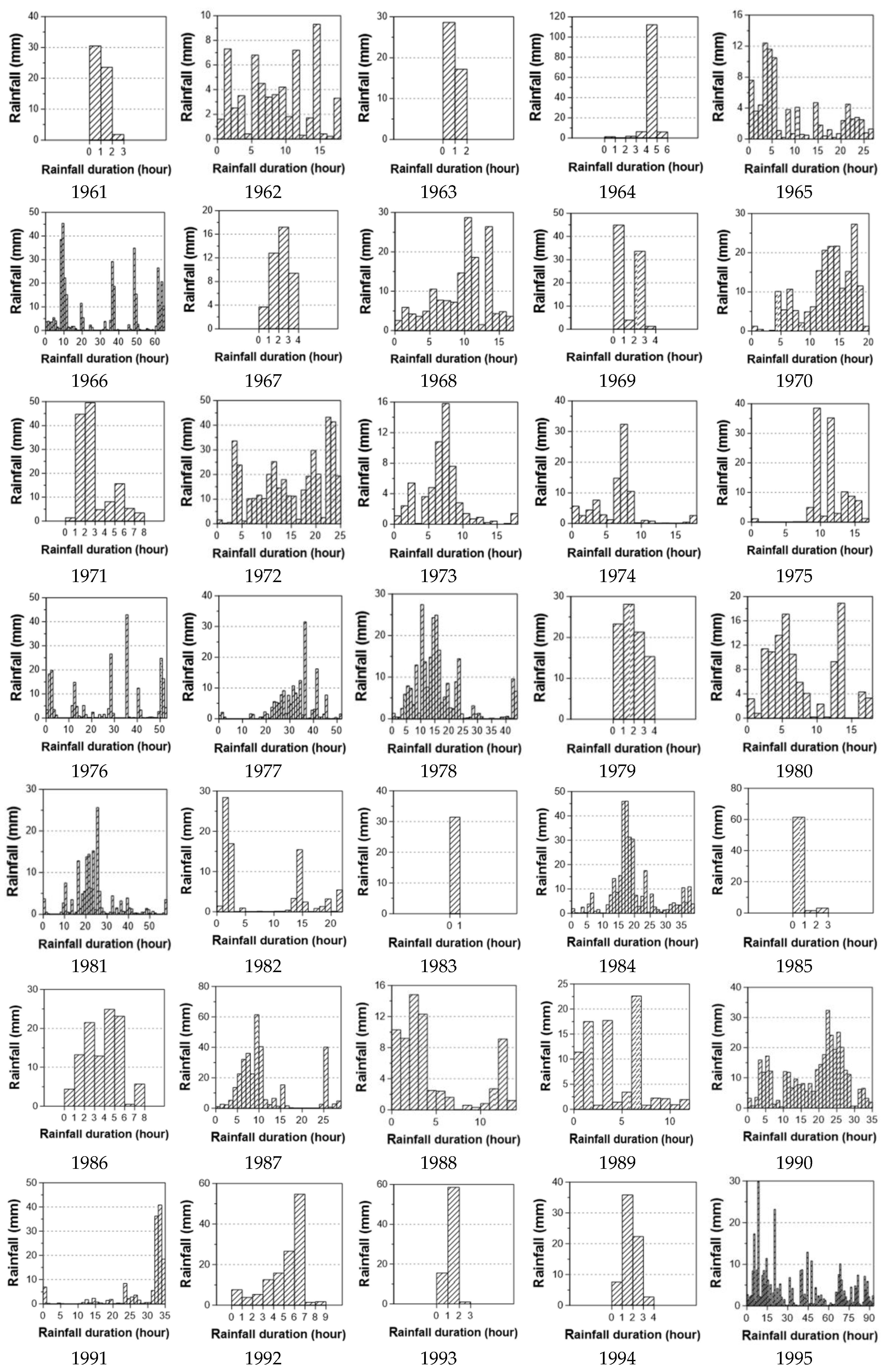
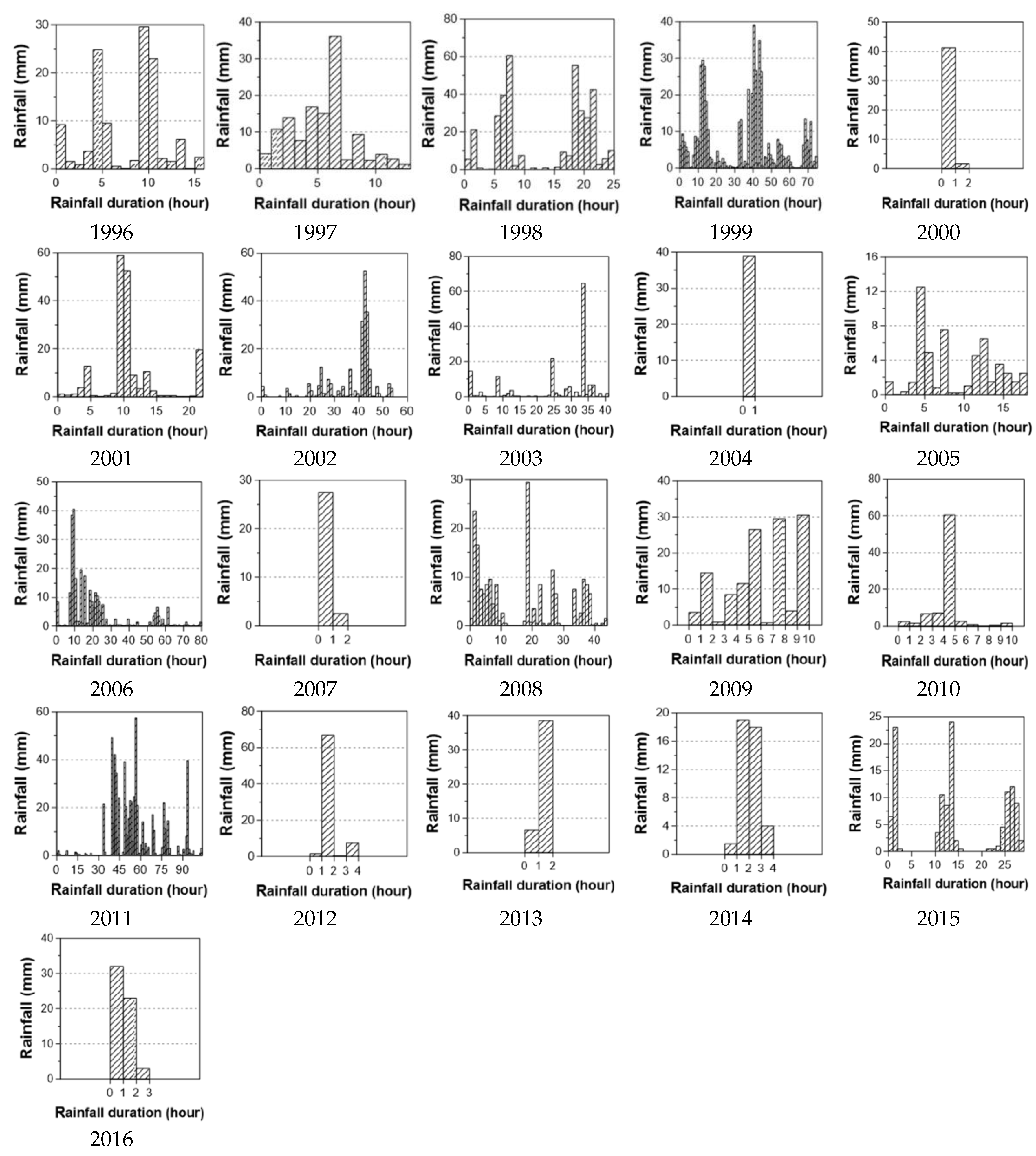
3.1. Data
3.2. Model Fitting
4. Evaluation of the Rainfall Temporal Distribution Models
4.1. Evaluation Methods and Evaluation Measures
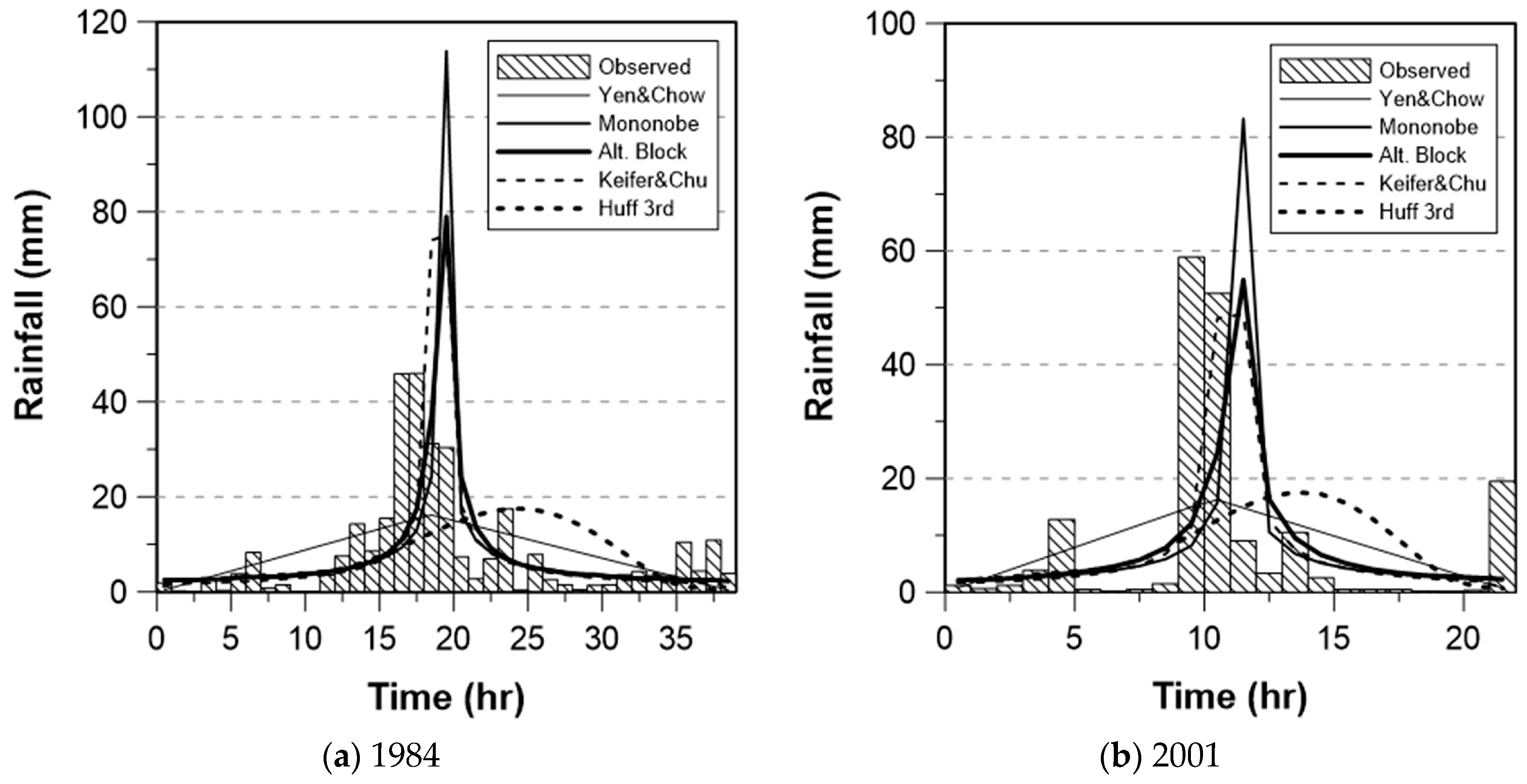
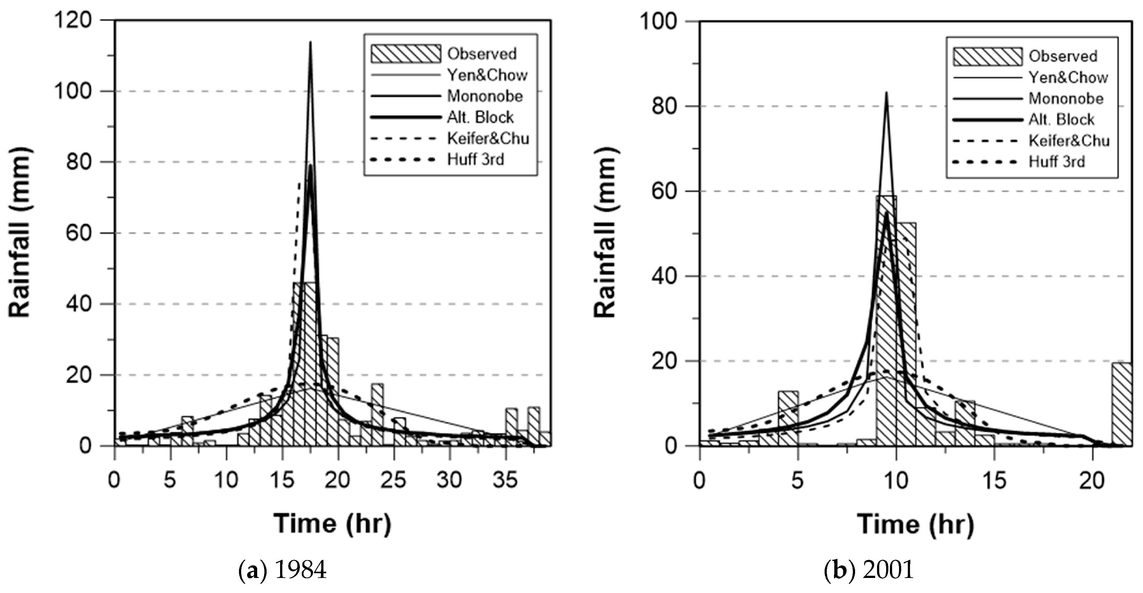
4.2. Evaluation Results
5. Sensitivity of the Runoff Peak to the Rainfall Temporal Distribution
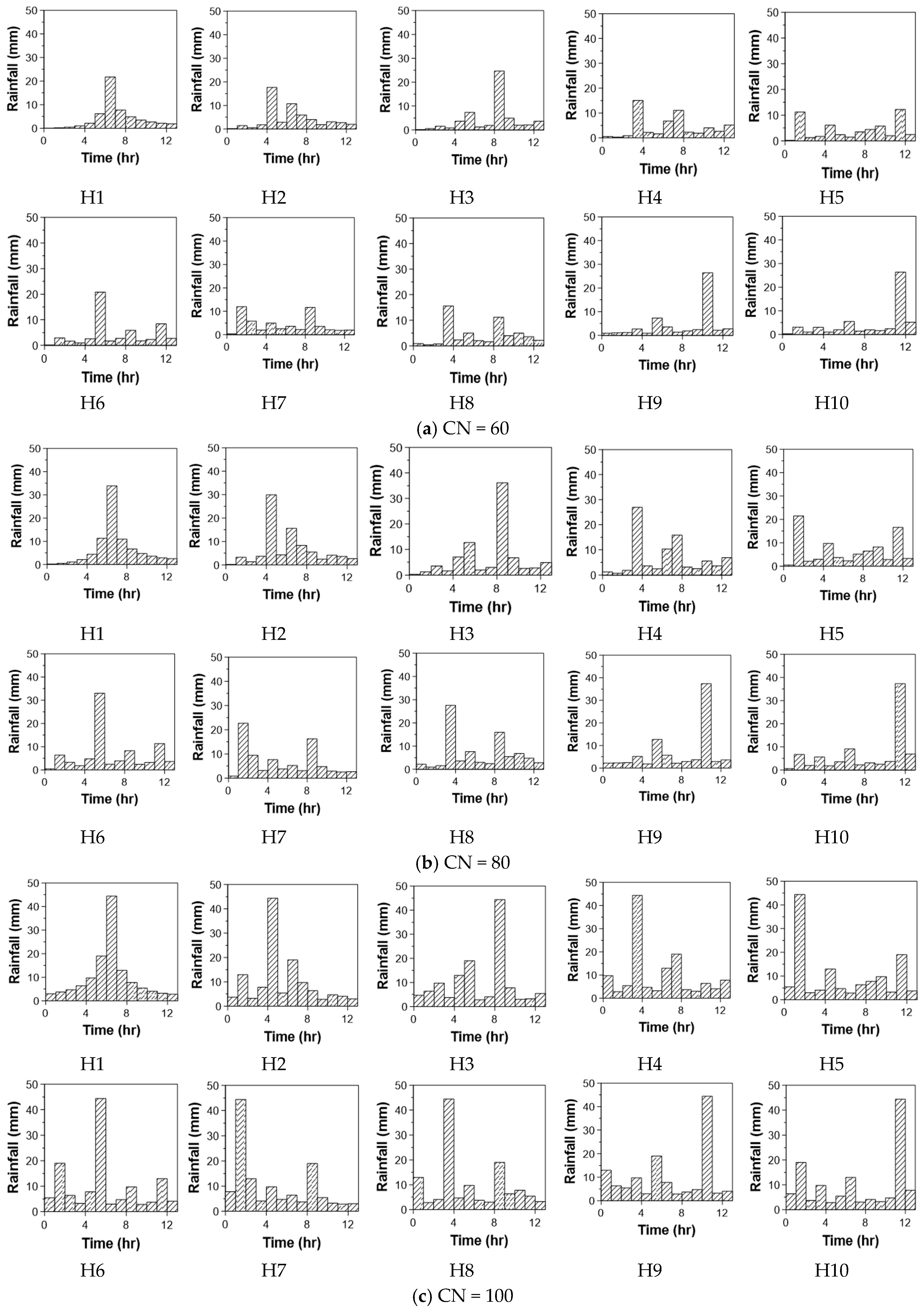
5.1. Preparation of the Rainfall–Runoff Model
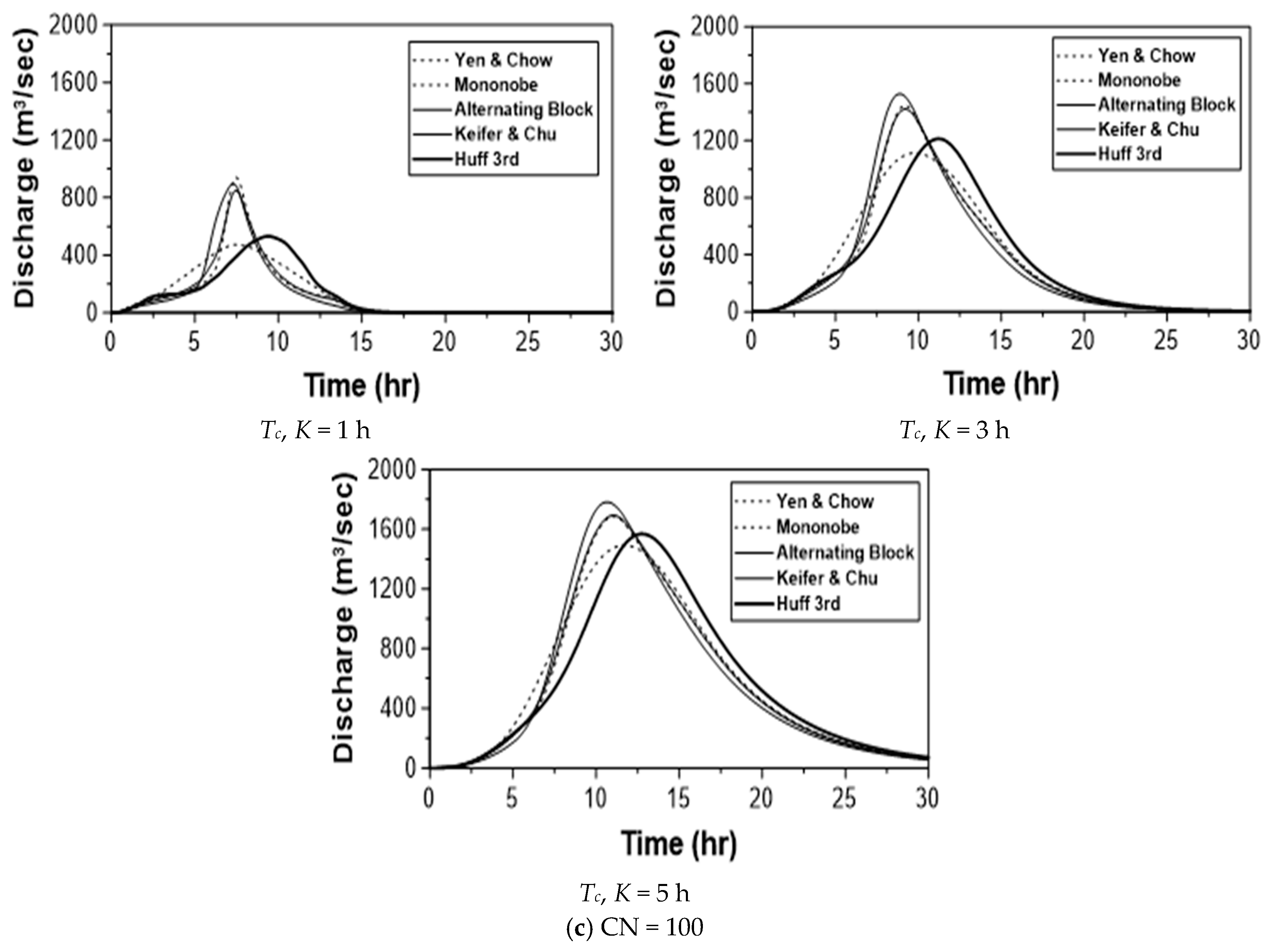
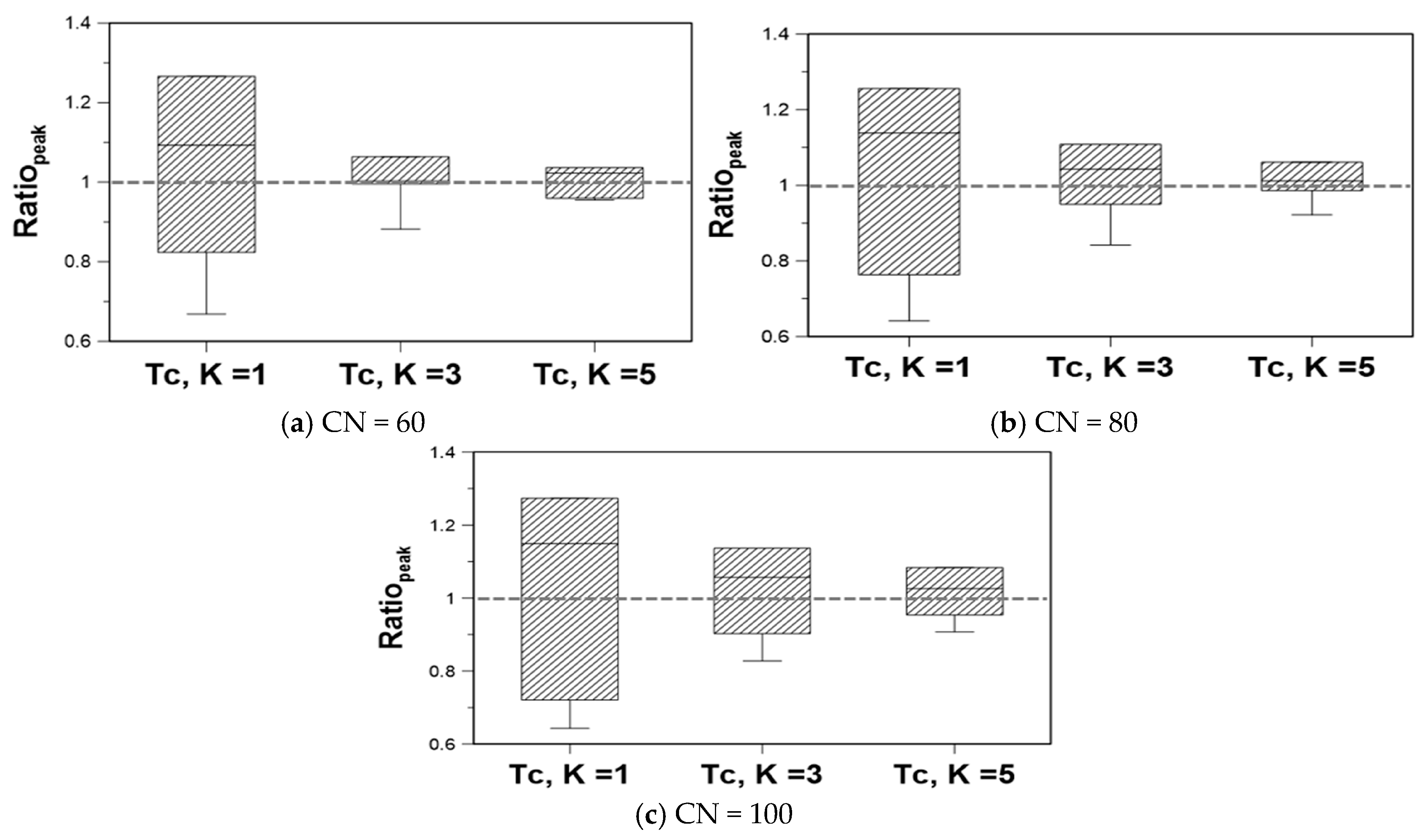
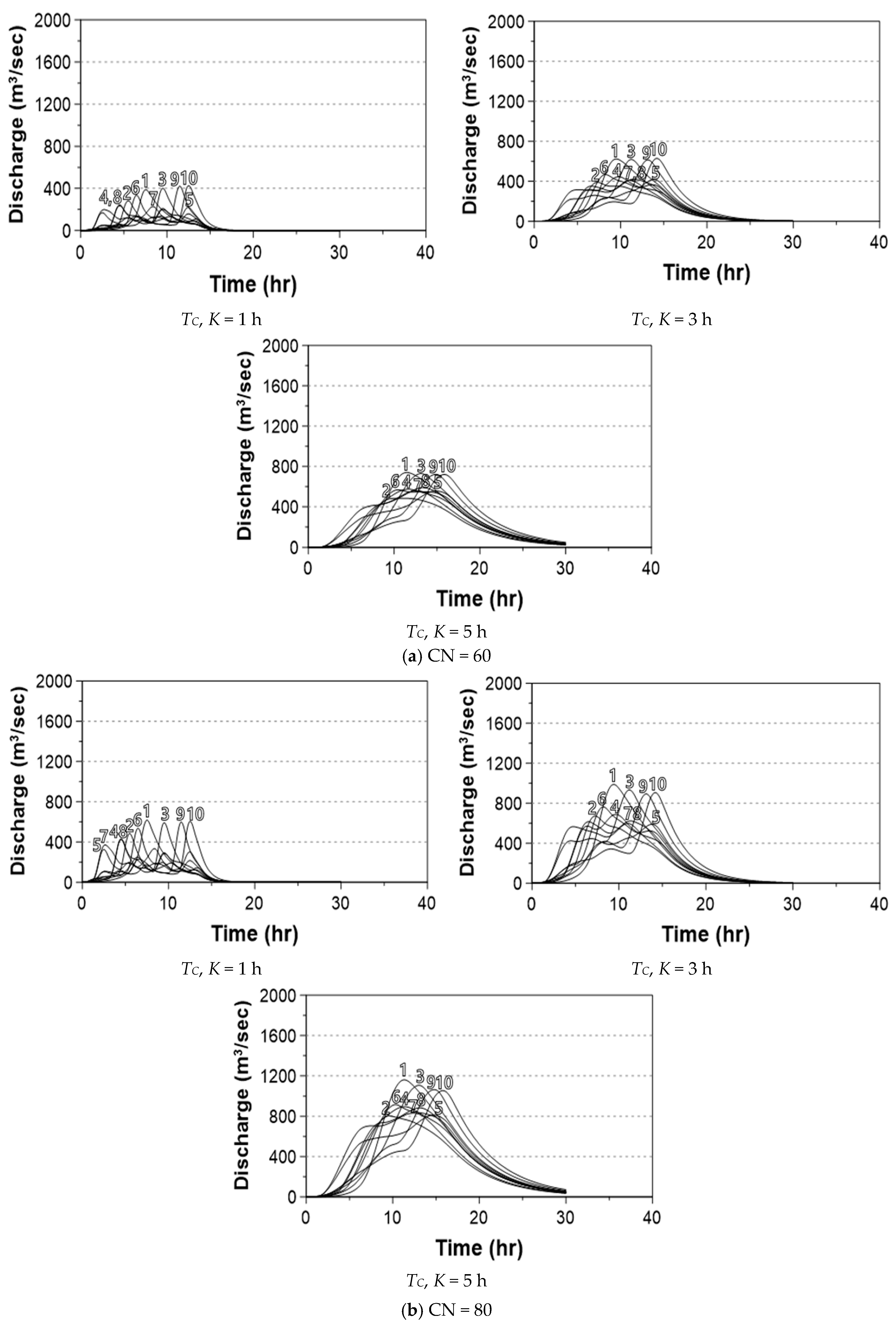
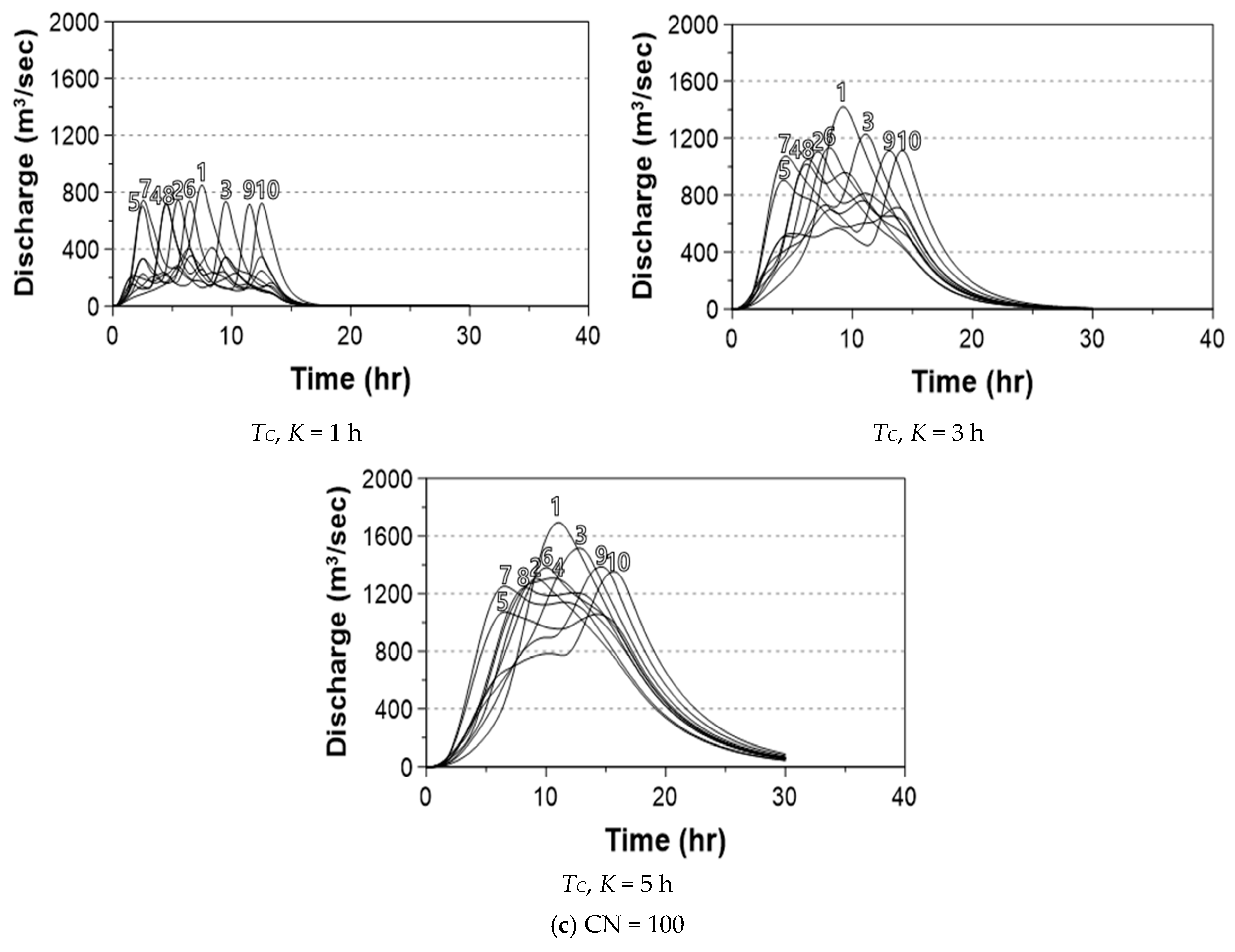
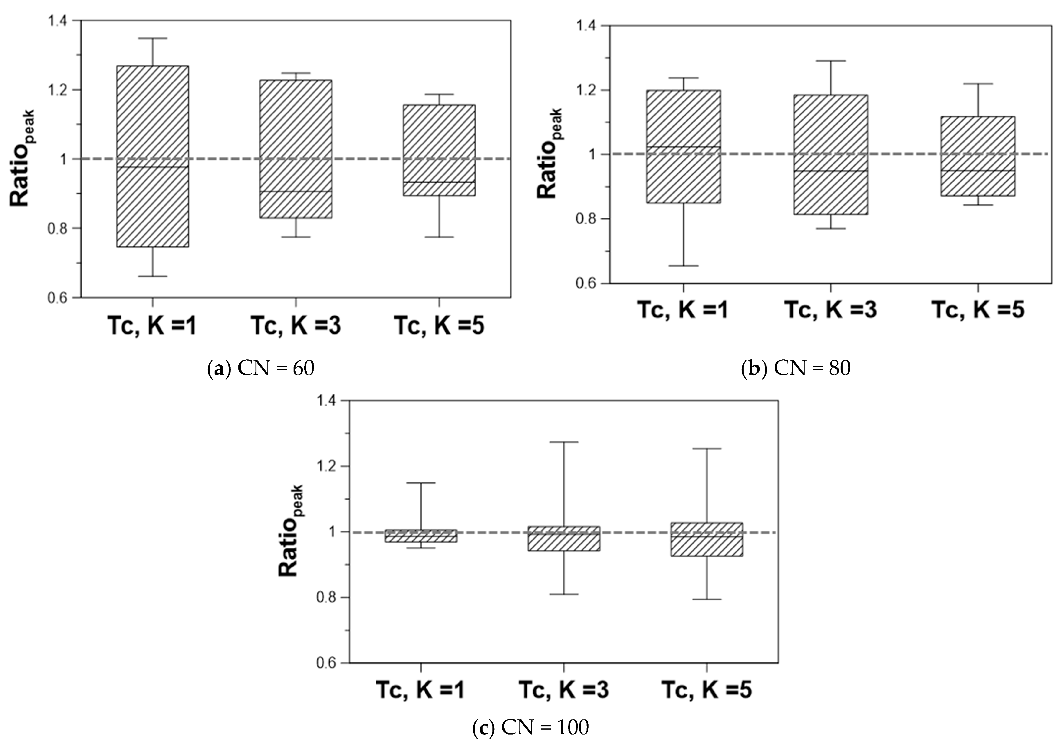
5.2. Sensitivity to the Rainfall Temporal Distribution Models
5.3. Preparation of the Rainfall–Runoff Model
6. Summary and Conclusions
Author Contributions
Funding
Conflicts of Interest
References
- Nouh, M.A. Effects of Rainfall Runoff Model Assumptions on Optimal Storm-Sewer System-Design. Arab. J. Sci. Eng. 1987, 12, 19–35. [Google Scholar]
- U.S. Soil Conservation Service (SCS). A Method for Estimating Volume and Rate of Runoff in Small Watersheds; U.S. Soil Conservation Service: Washington, DC, USA, 1973. [Google Scholar]
- Huff, F.A. Time Distribution of Rainfall in Heavy Storms. Water Resour. Res. 1967, 3, 1007–1019. [Google Scholar] [CrossRef]
- Jeong, J.H.; Yoon, Y.N. Design Practices for Water Resources; Goomi Press: Seoul, Korea, 2007. [Google Scholar]
- Pilgrim, D.H.; Cordery, I. Rainfall Temporal Patterns for Design Floods. J. Hydraul. Div. ASCE 1975, 101, 81–95. [Google Scholar]
- Yen, B.C.; Chow, V.T. Design Hyetographs for Small Drainage Structures. J. Hydraul. Div. ASCE 1980, 106, 1055–1076. [Google Scholar]
- Chow, V.T.; Maidment, D.R.; Mays, L.W. Applied Hydrology; McGraw-Hill: New York, NY, USA, 1988. [Google Scholar]
- Keifer, C.J.; Chu, H.H. Synthetic storm pattern for drainage design. J. Hydraul. Div. 1957, 83, 1–25. [Google Scholar]
- Lee, K.T.; Ho, J.Y. Design hyetograph for typhoon rainstorms in Taiwan. J. Hydrol. Eng. 2008, 13, 647–651. [Google Scholar] [CrossRef]
- Garcia-Guzman, A.; Aranda-Oliver, E. A Stochastic-Model of Dimensionless Hyetograph. Water Resour. Res. 1993, 29, 2363–2370. [Google Scholar] [CrossRef]
- Lin, G.F.; Chen, L.H.; Kao, S.C. Development of regional design hyetographs. Hydrol. Process. 2005, 19, 937–946. [Google Scholar] [CrossRef]
- Cheng, K.S.; Hueter, I.; Hsu, E.; Yen, H.C. A scale-invariant Gauss—Markov model for design storm hyetographs. J. Am. Water Resour. Assoc. 2001, 37, 723–735. [Google Scholar] [CrossRef]
- Wu, S.J.; Yang, J.C.; Tung, Y.K. Identification and stochastic generation of representative rainfall temporal patterns in Hong Kong territory. Stoch. Environ. Res. Risk Assess. 2006, 20, 171–183. [Google Scholar] [CrossRef]
- National Ocanic and Atmospheric Administration (NOAA). Precipitation-Frequency Atlas of the United States; NOAA: Silver Spring, MD, USA, 2013. [Google Scholar]
- Chan, E.S.; Balmforth, D.; Kan, Y.; Koike, T.; Lampe, L.; Lim, K.K.; Yong, K.K. Report on Key Conclusions and Recommendations of the Expert Panel on Drainage Design and Flood Protection Measures; Singapore’s National Water Agency: Singapore, 2012. [Google Scholar]
- Ministry of Construction and Transportation (MOCT). River Maintenance Basic Plan and Instructions of River Maintenance Report; MOCT: Seoul, Korea, 2004. [Google Scholar]
- Yin, S.Q.; Xie, Y.; Nearing, M.A.; Guo, W.L.; Zhu, Z.Y. Intra-Storm Temporal Patterns of Rainfall in China Using Huff Curves. Trans. ASABE 2016, 59, 1619–1632. [Google Scholar] [Green Version]
- Nelson City Council. Maitai River Flood Hazard Mapping Modelling Report; Nelson City Council: Nelson, New Zealand, 2013. [Google Scholar]
- Palla, A.; Gnecco, I. Assessing the urban catchment hydrologic response under different environmental scenarios. In Proceedings of the NOVATECH 2016—9th International Conference on Planning and Technologies for Sustainable Urban Water Management, Lyon, France, 28 June–1 July 2016. [Google Scholar]
- Japan International Cooperation Agency (JICA). Technical Standards and Guidelines for Planning of Flood Control Structures; JICA: Tokyo, Japan, 2010; pp. 39–42. [Google Scholar]
- Drainage Services Department. Stormwater Drainage Manual: Planning, Design and Management; Drainage Services Department: Hong Kong, China, 2018; Volume 26. [Google Scholar]
- Japanese Ministry of Land, Infrastructure, Transport and Tourism (MLITT); Kanazawa, H.; Yoshitani, J.; Shintaku, S. Technical Criteria for River Works: Practical Guide for Planning; MLITT: Tokyo, Japan, 2009. [Google Scholar]
- Al-Rawas, G.A.; Valeo, C. Characteristics of rainstorm temporal distributions in arid mountainous and coastal regions. J. Hydrol. 2009, 376, 318–326. [Google Scholar] [CrossRef]
- Aron, G.; Wall, D.J.; White, E.L.; Dunn, C.N. Regional Rainfall Intensity-Duration-Frequency Curves for Pennsylvania. Water Resour. Bull. 1987, 23, 479–485. [Google Scholar] [CrossRef]
- Guo, J.C.Y.; Hargadin, K. Conservative Design Rainfall Distribution. J. Hydrol. Eng. 2009, 14, 528–530. [Google Scholar] [CrossRef]
- Kimoto, A.; Canfield, H.E.; Stewart, D. Comparison of Synthetic Design Storms with Observed Storms in Southern Arizona. J. Hydrol. Eng. 2011, 16, 935–941. [Google Scholar] [CrossRef]
- Nguyen, V.T.V.; Desramaut, N.; Nguyen, T.D. Optimal rainfall temporal patterns for urban drainage design in the context of climate change. Water Sci. Technol. 2010, 62, 1170–1176. [Google Scholar] [CrossRef] [PubMed]
- Ministry of Construction and Transportation (MOCT). 1999 Report on the Development of Water Resources Management Techniques: Design Rainfall Temporal Distribution; MOCT: Seoul, Korea, 2000. [Google Scholar]
- Ministry of Land, Transport and Maritime Affairs (MLTM). Research on the Improvement of Probability Rainfall; MLTM: Seoul, Korea, 2011. [Google Scholar]
- Choi, S.; Joo, K.; Shin, H.; Heo, J. Improvement of Huff’s Method Considering Severe Rainstorm Events. J. Korea Water Resour. Assoc. 2014, 47, 985–996. [Google Scholar] [CrossRef]
- Joo, J.; Lee, J.; Jo, D.; Jun, H.; Kim, J. Development of a Rainfall Time Distribution Model for Urban Watersheds. J. Korea Water Resour. Assoc. 2007, 40, 655–663. [Google Scholar] [CrossRef] [Green Version]
- Knapp, H.V.; Terstriep, M.L. Effects of Basin Rainfall Estimates on Dam Safety Design in Illinois; Illinois State Water Survey: Champaign, IL, USA, 1981; pp. 14–22. [Google Scholar]
- Ward, A.B.; Bridges, T.; Barfield, B. An evaluation of hydrologic modeling techniques for determining a design storm hydrograph. In Proceedings of the International Symposium on Urban Storm Runoff, University of Kentucky, Lexington, Kentucky, 28–31 July 1980; pp. 28–31. [Google Scholar]
- Lee, J.K.; Chu, H.J. Time distribution characteristics of an annual maximum rainfall according to rainfall durations using Huff’s method. J. Korean Soc. Civ. Eng. 2006, 26, 519–528. [Google Scholar]
- Park, M.; Yoo, C.; Kim, H.; Jun, C. Bivariate frequency analysis of annual maximum rainfall event series in Seoul, Korea. J. Hydrol. Eng. 2014, 19, 1080–1088. [Google Scholar] [CrossRef]
- Park, C.; Yoo, C. Review of parameter estimation procedure of Freud bivariate exponential distribution. J. Korea Water Resour. Assoc. 2012, 45, 191–201. [Google Scholar] [CrossRef]
- Loveridge, M.; Babister, M.; Retallick, M. Australian Rainfall and Runoff Revision Project 3: Temporal Patterns of Rainfall; Department of Industry, Innovation and Science: Canberra, Australia, 2015. [Google Scholar]
- Mockus, V. National Engineering Handbook: Section 4, Hydrology; U.S. Department of Agriculture: Washington, DC, USA, 1965. [Google Scholar]


| Year | Rainfall Duration (h) | Rainfall Depth (mm) | Rainfall Intensity (mm/h) | Year | Rainfall Duration (h) | Rainfall Depth (mm) | Rainfall Intensity (mm/h) |
|---|---|---|---|---|---|---|---|
| 1961 | 3 | 55.9 | 18.6 | 1989 | 12 | 82.7 | 6.9 |
| 1962 | 18 | 62.0 | 3.4 | 1990 | 35 | 352.2 | 10.1 |
| 1963 | 2 | 45.8 | 22.9 | 1991 | 35 | 138.1 | 3.9 |
| 1964 | 6 | 127.4 | 21.2 | 1992 | 9 | 129.5 | 14.4 |
| 1965 | 27 | 87.0 | 3.2 | 1993 | 3 | 75.0 | 25.0 |
| 1966 | 65 | 361.7 | 5.6 | 1994 | 4 | 68.4 | 17.1 |
| 1967 | 4 | 43.1 | 10.8 | 1995 | 93 | 331.8 | 3.6 |
| 1968 | 17 | 156.7 | 9.2 | 1996 | 16 | 116.5 | 7.3 |
| 1969 | 4 | 83.7 | 20.9 | 1997 | 13 | 126.3 | 9.7 |
| 1970 | 20 | 191.8 | 9.6 | 1998 | 25 | 359.7 | 14.4 |
| 1971 | 8 | 132.8 | 16.6 | 1999 | 75 | 500.3 | 6.7 |
| 1972 | 25 | 394.5 | 15.8 | 2000 | 2 | 42.9 | 21.5 |
| 1973 | 18 | 59.5 | 3.3 | 2001 | 22 | 180.3 | 8.2 |
| 1974 | 18 | 87.0 | 4.8 | 2002 | 54 | 227.9 | 4.2 |
| 1975 | 17 | 112.1 | 6.6 | 2003 | 41 | 159.5 | 3.9 |
| 1976 | 53 | 226.3 | 4.3 | 2004 | 1 | 38.9 | 38.9 |
| 1977 | 52 | 168.2 | 3.2 | 2005 | 18 | 52.8 | 2.9 |
| 1978 | 44 | 244.3 | 5.6 | 2006 | 80 | 281.3 | 3.5 |
| 1979 | 4 | 88.0 | 22.0 | 2007 | 2 | 30.0 | 15.0 |
| 1980 | 18 | 116.0 | 6.4 | 2008 | 44 | 192.2 | 4.4 |
| 1981 | 58 | 156.2 | 2.7 | 2009 | 10 | 129.8 | 13.0 |
| 1982 | 22 | 80.2 | 3.6 | 2010 | 10 | 83.5 | 8.4 |
| 1983 | 1 | 31.4 | 31.4 | 2011 | 104 | 630.0 | 6.1 |
| 1984 | 39 | 317.5 | 8.1 | 2012 | 4 | 76.5 | 19.1 |
| 1985 | 3 | 66.0 | 22.0 | 2013 | 2 | 45.0 | 22.5 |
| 1986 | 8 | 106.2 | 13.3 | 2014 | 4 | 42.5 | 10.6 |
| 1987 | 29 | 323.8 | 11.2 | 2015 | 29 | 119.5 | 4.1 |
| 1988 | 14 | 67.8 | 4.8 | 2016 | 3 | 58.0 | 19.3 |
| Evaluation Measure | Year | Case | Yen and Chow | Mononobe | Alternating Block | Keifer and Chu | Huff |
|---|---|---|---|---|---|---|---|
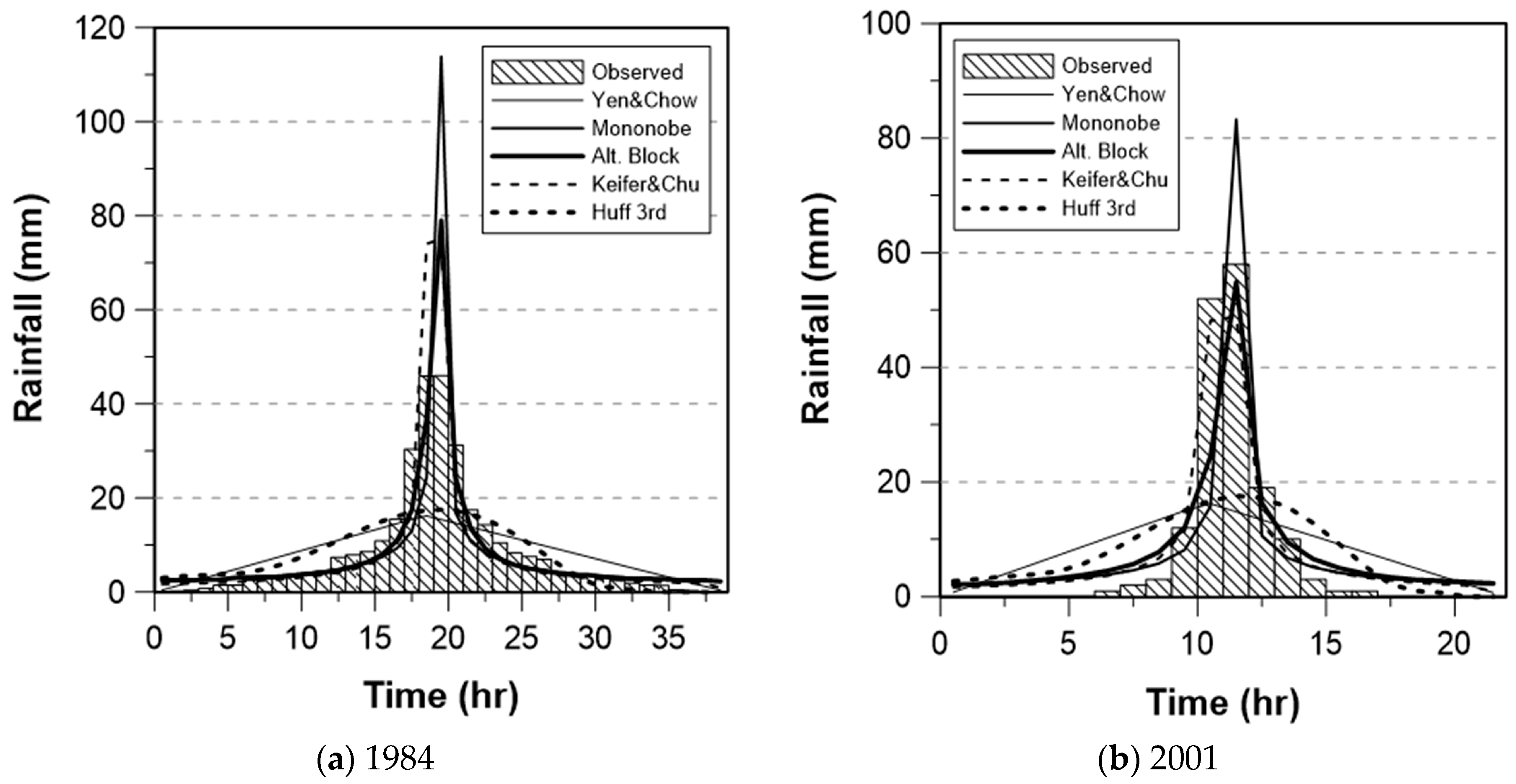
| DRpeak | 1984 | - | −29.8 | 67.8 | 33.0 | 29.0 | −28.5 |
| 2001 | - | −42.7 | 24.4 | −4.0 | −10.0 | −41.3 | |
| RMSE | 1984 | 1 | 9.45 | 16.13 | 11.73 | 13.17 | 11.47 |
| 2 | 9.51 | 12.86 | 6.57 | 8.44 | 9.48 | ||
| 3 | 8.30 | 12.20 | 6.32 | 7.53 | 8.13 | ||
| 2001 | 1 | 14.28 | 21.34 | 16.27 | 14.34 | 15.79 | |
| 2 | 14.05 | 11.89 | 10.55 | 4.81 | 14.62 | ||
| 3 | 13.33 | 9.93 | 6.57 | 3.35 | 13.05 | ||
| R | 1984 | 1 | 0.58 | 0.45 | 0.56 | 0.58 | 0.24 |
| 2 | 0.59 | 0.70 | 0.83 | 0.86 | 0.61 | ||
| 3 | 0.77 | 0.73 | 0.88 | 0.90 | 0.79 | ||
| 2001 | 1 | 0.46 | 0.14 | 0.33 | 0.52 | 0.19 | |
| 2 | 0.45 | 0.73 | 0.73 | 0.92 | 0.50 | ||
| 3 | 0.64 | 0.82 | 0.93 | 0.99 | 0.50 |
| Evaluation Measure | Case | Yen and Chow | Mononobe | Alternating Block | Keifer and Chu | Huff |
|---|---|---|---|---|---|---|
| SDRpeak | - | −0.499 | 0.706 | 0.548 | 0.473 | −0.467 |
| (0.240) | (0.593) | (0.453) | (0.419) | (0.245) | ||
| SRMSE | 1 | 1.337 | 1.894 | 1.810 | 2.012 | 1.398 |
| (0.592) | (0.731) | (0.793) | (1.000) | (0.572) | ||
| 2 | 1.242 | 1.299 | 1.296 | 1.592 | 1.189 | |
| (0.628) | (0.629) | (0.717) | (0.986) | (0.616) | ||
| 3 | 0.955 | 0.914 | 0.754 | 1.135 | 1.039 | |
| (0.557) | (0.310) | (0.386) | (0.794) | (0.544) | ||
| R | 1 | 0.268 | 0.208 | 0.238 | 0.304 | 0.170 |
| (0.337) | (0.264) | (0.259) | (0.266) | (0.350) | ||
| 2 | 0.508 | 0.733 | 0.732 | 0.610 | 0.541 | |
| (0.304) | (0.173) | (0.196) | (0.252) | (0.285) | ||
| 3 | 0.751 | 0.804 | 0.877 | 0.743 | 0.629 | |
| (0.171) | (0.126) | (0.100) | (0.201) | (0.207) |
| Model | CN | Tc = K (h) |
|---|---|---|
| Yen and Chow | 60 | 1 |
| Mononobe | ||
| Alternating Block | 80 | 3 |
| Keifer and Chu | 100 | 5 |
| Huff |
© 2018 by the authors. Licensee MDPI, Basel, Switzerland. This article is an open access article distributed under the terms and conditions of the Creative Commons Attribution (CC BY) license (http://creativecommons.org/licenses/by/4.0/).
Share and Cite
Na, W.; Yoo, C. Evaluation of Rainfall Temporal Distribution Models with Annual Maximum Rainfall Events in Seoul, Korea. Water 2018, 10, 1468. https://doi.org/10.3390/w10101468
Na W, Yoo C. Evaluation of Rainfall Temporal Distribution Models with Annual Maximum Rainfall Events in Seoul, Korea. Water. 2018; 10(10):1468. https://doi.org/10.3390/w10101468
Chicago/Turabian StyleNa, Wooyoung, and Chulsang Yoo. 2018. "Evaluation of Rainfall Temporal Distribution Models with Annual Maximum Rainfall Events in Seoul, Korea" Water 10, no. 10: 1468. https://doi.org/10.3390/w10101468