Contrasting Responses among Aquatic Organism Groups to Changes in Geomorphic Complexity Along a Gradient of Stream Habitat Restoration: Implications for Restoration Planning and Assessment

 , , ,
, , ,
Abstract
:1. Introduction
2. Methods
2.1. Study Area
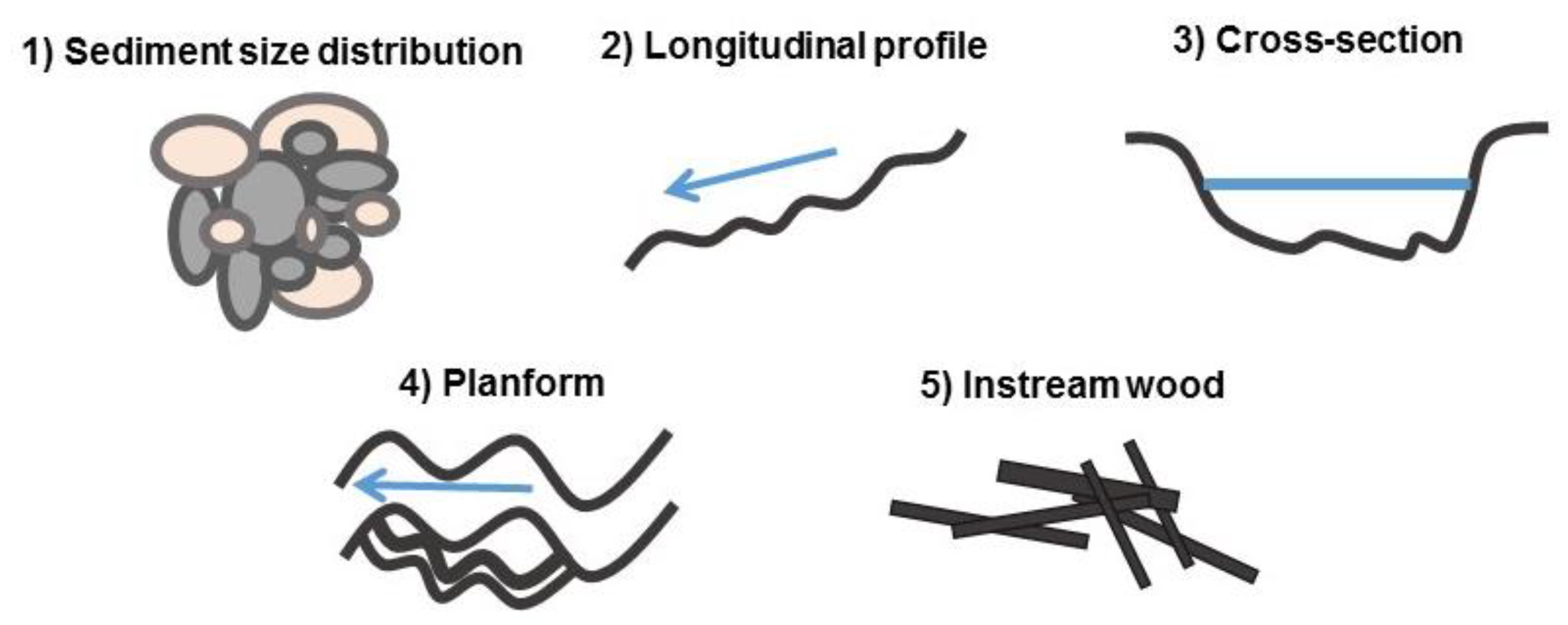
2.2. Geomorphic Complexity Metrics
2.3. Site Characteristics
2.4. Biotic Sampling
2.4.1. Macroinvertebrates
2.4.2. Diatoms and Other Periphyton
2.4.3. Macrophytes
2.5. Data Analysis
3. Results
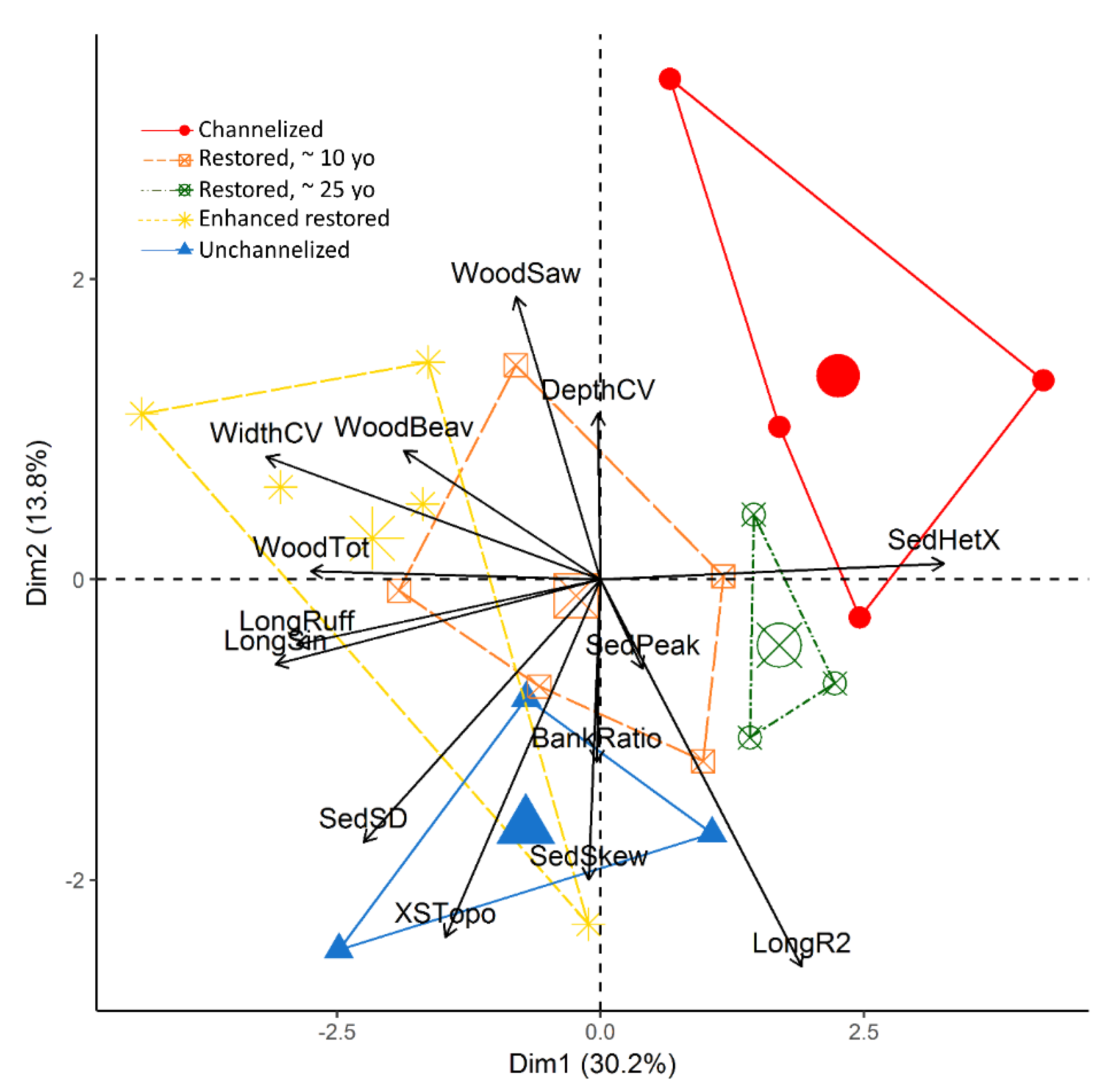
3.1. Geomorphic Complexity
3.2. Other Stream Reach Characteristics
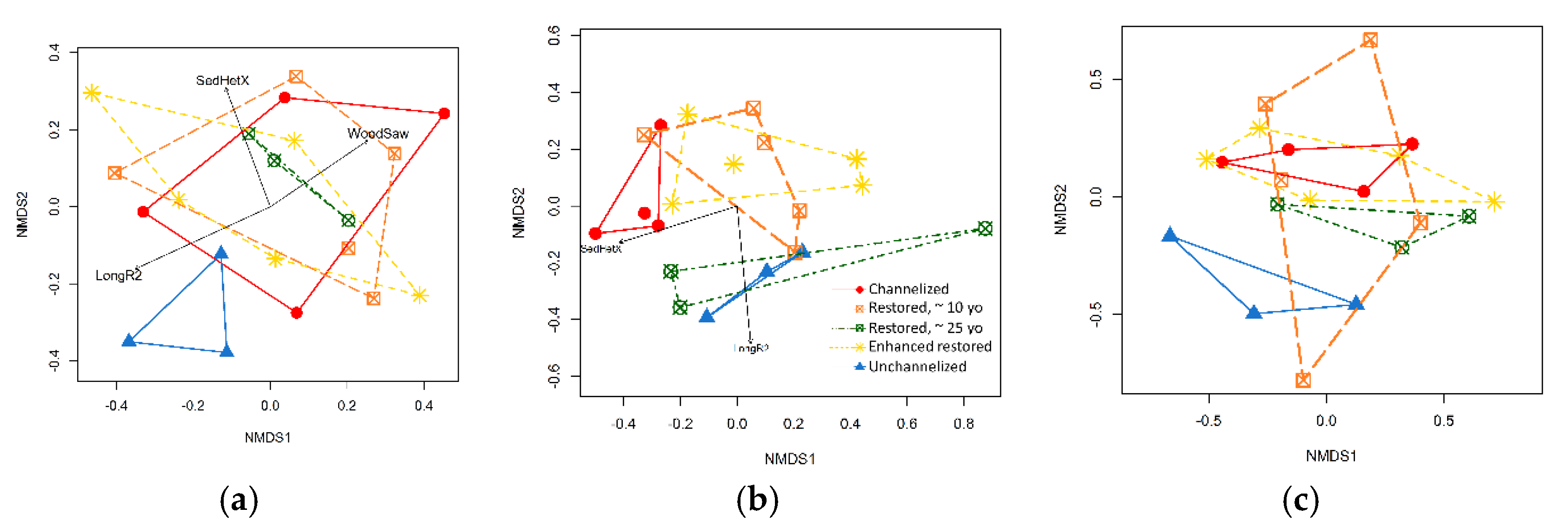
3.3. Diversity and Community Composition of Three Organism Groups
3.3.1. Macroinvertebrates
3.3.2. Diatoms
3.3.3. Macrophytes
4. Discussion
4.1. Macroinvertebrates
4.2. Diatoms
4.3. Macrophytes
4.4. A Gradient in Complexity/Restoration Effort
4.5. Implications for Restoration Practice
Author Contributions
Funding
Acknowledgments
Conflicts of Interest
Appendix A. Correlation Matrix for Geomorphic Complexity Metrics

| Complexity Metric | Sediment Distribution | Longitudinal Profile | Cross-Section | Planform | Instream Wood | |||||||||
|---|---|---|---|---|---|---|---|---|---|---|---|---|---|---|
| Het2 | Sort | Kurt | Skew | LP_R2 | Rough | Thal_P | XS_CT | XS_CV_d | W_cv | Bratio | WV_tot | WV_beav | WV_saw | |
| Het2 | 1.00 | −0.36 | 0.13 | 0.05 | 0.36 | −0.63 | −0.77 | −0.25 | 0.04 | −0.71 | −0.11 | −0.57 | −0.29 | −0.02 |
| Sort | 1.00 | −0.03 | 0.05 | 0.08 | 0.69 | 0.36 | 0.47 | −0.16 | 0.35 | −0.04 | 0.50 | −0.08 | 0.11 | |
| Kurt | 1.00 | 0.38 | −0.01 | −0.21 | 0.08 | 0.10 | 0.17 | −0.02 | −0.09 | −0.08 | −0.25 | 0.12 | ||
| Skew | 1.00 | 0.16 | −0.01 | 0.10 | 0.28 | −0.06 | −0.08 | 0.01 | 0.10 | 0.22 | −0.25 | |||
| LP_R2 | 1.00 | −0.35 | −0.24 | 0.05 | −0.32 | −0.50 | 0.24 | −0.29 | −0.44 | −0.37 | ||||
| Rough | 1.00 | 0.44 | 0.25 | 0.03 | 0.49 | 0.06 | 0.51 | 0.10 | 0.11 | |||||
| Thal_P | 1.00 | 0.35 | −0.20 | 0.69 | 0.00 | 0.51 | 0.40 | 0.06 | ||||||
| XS_CT | 1.00 | −0.03 | 0.18 | 0.17 | 0.08 | 0.30 | −0.26 | |||||||
| XS_CV_d | 1.00 | 0.04 | −0.03 | 0.13 | 0.19 | −0.28 | ||||||||
| W_cv | 1.00 | 0.06 | 0.46 | 0.45 | 0.33 | |||||||||
| Bratio | 1.00 | −0.01 | −0.16 | −0.01 | ||||||||||
| WV_tot | 1.00 | 0.30 | 0.16 | |||||||||||
| WV_beav | 1.00 | 0.02 | ||||||||||||
| WV_saw | 1.00 | |||||||||||||
Appendix B. Differences for Site Characteristics among the Restoration Statuses
| Site Characteristics | Reference | Control | Categories of Restored Sites | χ2 | p | ||||||||||||
|---|---|---|---|---|---|---|---|---|---|---|---|---|---|---|---|---|---|
| Unchannelized | Channelized | Enhanced 2-Year-Old | Best-Practice 10-Year-Old | Best-Practice 25-Year-Old | |||||||||||||
| Total N (µg/L) | 261.33 | ± | 25.57 | 276.38 | ± | 27.89 | 259.50 | ± | 16.50 | 257.58 | ± | 16.92 | 242.50 | ± | 15.50 | 2.934 | 0.569 |
| NH4 (µg/L) | 5.033 | ± | 1.467 a,b | 4.250 | ± | 0.595 b | 5.600 | ± | 0.332 a,b | 5.500 | ± | 0.563 a,b | 8.500 | ± | 0.500 a | 12.22 | 0.016 |
| NO3 (µg/L) | 9.500 | ± | 3.606 | 6.875 | ± | 2.511 | 5.800 | ± | 2.077 | 3.917 | ± | 0.970 | 3.500 | ± | 0.500 | 5.748 | 0.219 |
| pH | 7.197 | ± | 0.048 | 7.960 | ± | 0.557 | 7.412 | ± | 0.214 | 7.632 | ± | 0.270 | 7.920 | ± | 0.840 | 4.902 | 0.298 |
| DOC (Absorbance-F4205) | 0.143 | ± | 0.015 a | 0.093 | ± | 0.015 a,b | 0.094 | ± | 0.011 b | 0.102 | ± | 0.011 a,b | 0.133 | ± | 0.015 a,b | 12.12 | 0.016 |
| Drainage area (km2) | 27.12 | ± | 8.92 | 128.20 | ± | 60.24 | 75.18 | ± | 24.80 | 56.55 | ± | 26.25 | 37.23 | ± | 2.96 | 4.343 | 0.362 |
| Latitude (DD) | 64.85 | ± | 0.37 | 65.13 | ± | 0.13 | 65.06 | ± | 0.08 | 64.99 | ± | 0.10 | 64.56 | ± | 0.03 | 6.987 | 0.137 |
| Longitude (DD) | 18.76 | ± | 0.56 | 18.11 | ± | 0.09 | 18.32 | ± | 0.08 | 18.37 | ± | 0.12 | 18.82 | ± | 0.11 | 8.927 | 0.063 |
| Stream depth (cm) | 36.02 | ± | 5.97 | 38.38 | ± | 1.79 | 38.36 | ± | 3.94 | 33.65 | ± | 3.52 | 30.33 | ± | 3.18 | 3.436 | 0.488 |
| Stream slope (m/m) | 0.037 | ± | 0.004 a | 0.008 | ± | 0.002 b | 0.020 | ± | 0.004 a,b | 0.013 | ± | 0.004 b | 0.015 | ± | 0.007 a,b | 16.59 | 0.002 |
| Riparian buffer width (m) | 70.00 | ± | 24.02 | 52.75 | ± | 22.65 | 23.88 | ± | 8.85 | 24.36 | ± | 4.71 | 15.19 | ± | 7.44 | 6.499 | 0.165 |
| Leaf Area Index | 1.353 | ± | 0.194 a | 0.570 | ± | 0.131 c | 0.578 | ± | 0.112 c | 0.706 | ± | 0.110 b,c | 1.256 | ± | 0.135 a,b | 19.70 | 0.001 |
| Distance to lake (km) | 1.520 | ± | 0.427 | 0.988 | ± | 0.424 | 1.000 | ± | 0.415 | 0.825 | ± | 0.426 | 0.310 | ± | 0.080 | 5.262 | 0.262 |
| N | 3 | 4 | 5 | 5 | 3 | ||||||||||||
Appendix C. Differences among Restoration Statuses for Species Richness, Shannon Index, and Abundance of the Three Organism Groups
| Taxonomic Group | Metric | Reference | Control | Categories of Restored Sites | χ2 | p | ||||||||||||
|---|---|---|---|---|---|---|---|---|---|---|---|---|---|---|---|---|---|---|
| Unchannelized | Channelized | Enhanced 2-Year-Old | Best-Practice 10-Year-Old | Best-Practice 25-Year-Old | ||||||||||||||
| Macroinvertebrate | Species richness † | 31.33 | ± | 2.33 | 30.75 | ± | 2.56 | 31.60 | ± | 1.69 | 35.20 | ± | 3.83 | 30.67 | ± | 2.19 | 1.369 | 0.850 |
| Shannon index | 2.59 | ± | 0.06 | 2.44 | ± | 0.14 | 2.45 | ± | 0.16 | 2.41 | ± | 0.13 | 2.59 | ± | 0.08 | 1.869 | 0.760 | |
| Abundance (#) † | 1890.00 | ± | 501.27 | 2490.21 | ± | 1522.56 | 2186.00 | ± | 1027.77 | 3129.60 | ± | 941.89 | 1525.33 | ± | 112.96 | 0.880 | 0.927 | |
| Diatom | Species richness † | 37.33 | ± | 3.71 | 31.25 | ± | 2.75 | 30.80 | ± | 4.81 | 32.80 | ± | 5.47 | 26.67 | ± | 0.33 | 2.769 | 0.597 |
| Shannon index | 3.70 | ± | 0.27 | 4.00 | ± | 0.23 | 3.31 | ± | 0.33 | 3.26 | ± | 0.24 | 3.09 | ± | 0.49 | 5.528 | 0.237 | |
| Biovolume (μm3/cm2) ‡ | 11.67 | ± | 3.84 | 13.75 | ± | 2.02 | 11.20 | ± | 2.20 | 6.80 | ± | 3.46 | 10.00 | ± | 3.51 | 3.786 | 0.436 | |
| IPS index | 19.53 | ± | 0.22 | 19.60 | ± | 0.13 | 19.68 | ± | 0.09 | 19.76 | ± | 0.09 | 19.43 | ± | 0.42 | 2.228 | 0.694 | |
| ACID index | 5.10 | ± | 0.30 | 4.53 | ± | 0.26 | 5.42 | ± | 0.56 | 5.28 | ± | 0.43 | 5.10 | ± | 1.10 | 1.708 | 0.789 | |
| Macrophyte | Species richness | 5.67 | ± | 0.88 | 7.50 | ± | 1.44 | 7.20 | ± | 0.86 | 7.20 | ± | 1.07 | 5.33 | ± | 2.03 | 2.000 | 0.736 |
| Shannon index | 0.538 | ± | 0.187 | 0.581 | ± | 0.140 | 0.682 | ± | 0.174 | 0.774 | ± | 0.125 | 0.467 | ± | 0.257 | 2.369 | 0.668 | |
| Percent cover † | 26.15 | ± | 12.60 | 16.09 | ± | 7.01 | 4.31 | ± | 1.50 b | 7.97 | ± | 2.03 a | 34.25 | ± | 15.95 | 13.02 | 0.011 | |
| N | 3 | 4 | 5 | 5 | 3 | |||||||||||||
Appendix D. SIMPER Analysis of Benthic Macroinvertebrate Taxa
| Taxon | FFG | Taxonomic Affinity | Average Dissimilarity | % Contribution | Cumulative % | Mean Abundance for Restoration Statuses | ||||
|---|---|---|---|---|---|---|---|---|---|---|
| Unchan | Chan | E | 10yo | 25yo | ||||||
| Pisidium spp. | Collector-filterer | V | 1.43 | 3.22 | 3.22 | 91.70 | 99.60 | 247.00 | 472.00 | 256.00 |
| Hydropsyche siltalai | Collector-filterer | T | 1.35 | 3.04 | 6.26 | 0.83 | 30.20 | 478.00 | 201.00 | 100.00 |
| Ephemerella spp. | Collector-gatherer | E | 1.26 | 2.84 | 9.09 | 38.30 | 148.00 | 71.00 | 31.40 | 1.33 |
| Elmis aenea | Scraper | C | 1.20 | 2.70 | 11.79 | 331.00 | 4.92 | 6.40 | 40.80 | 1.33 |
| Heptagenia sulphurea | Scraper | E | 1.10 | 2.48 | 14.28 | 10.00 | 14.50 | 86.40 | 44.60 | 68.00 |
| Leptophlebia sp. | Gatherer | E | 1.09 | 2.46 | 16.73 | 0.83 | 27.50 | 16.10 | 44.00 | 25.30 |
| Neureclipsis bimaculata | Predator | T | 1.07 | 2.41 | 19.14 | 0.00 | 243.00 | 3.50 | 124.00 | 1.33 |
| Hydropsyche pellucidula | Collector-filterer | T | 1.06 | 2.38 | 21.53 | 0.00 | 79.50 | 39.80 | 19.60 | 9.33 |
| Protonemura meyeri | Shredder | P | 1.03 | 2.33 | 23.86 | 103.00 | 3.33 | 10.00 | 5.20 | 47.30 |
| Amphinemura borealis | Shredder | P | 1.03 | 2.32 | 26.18 | 40.00 | 3.75 | 34.80 | 11.00 | 9.33 |
| Polycentropus flavomaculatus | Predator | T | 1.00 | 2.27 | 28.44 | 0.00 | 39.60 | 5.10 | 73.00 | 25.30 |
| Nemoura flexuosa | Shredder | P | 1.00 | 2.26 | 30.71 | 31.70 | 0.83 | 12.60 | 4.80 | 20.00 |
| Leuctra digitata/hippopus | Shredder | P | 0.99 | 2.23 | 32.93 | 55.80 | 32.90 | 36.00 | 39.60 | 3.33 |
| Tanytarsini | Collector-gatherer | D | 0.95 | 2.13 | 35.07 | 93.30 | 864.00 | 173.00 | 904.00 | 175.00 |
| Taeniopteryx nebulosa | Shredder | P | 0.94 | 2.12 | 37.19 | 18.30 | 24.30 | 10.00 | 8.00 | 0.00 |
| Lepidostoma hirtum | Shredder | T | 0.91 | 2.06 | 39.25 | 5.83 | 4.17 | 10.70 | 7.00 | 31.30 |
| Oligochaeta | Collector-gatherer | O | 0.88 | 1.98 | 41.23 | 12.50 | 111.00 | 21.10 | 12.00 | 10.70 |
| Ceratopogonidae | Predator | D | 0.87 | 1.97 | 43.20 | 20.00 | 1.46 | 14.90 | 20.40 | 10.70 |
| Heptagenia dalecarlica | Scrapers | E | 0.87 | 1.97 | 45.17 | 0.00 | 21.70 | 13.40 | 5.40 | 0.00 |
| Isoperla sp. | Predator | P | 0.86 | 1.93 | 47.10 | 11.70 | 12.80 | 29.40 | 19.20 | 14.00 |
| Nigrobaetis niger | Scraper | E | 0.84 | 1.90 | 48.99 | 77.50 | 51.10 | 30.10 | 31.40 | 107.00 |
| Nigrobaetis digitatus | Scraper | E | 0.84 | 1.89 | 50.88 | 5.00 | 6.88 | 10.20 | 77.00 | 0.00 |
Appendix E. SIMPER Analysis of Diatom Taxa
| Taxon | Code | Ph * | Moisture † | Current ‡ | Life Form | Average Dissimilarity | % Contribution | Cumulative % | Mean Percent for Restoration Status | ||||
|---|---|---|---|---|---|---|---|---|---|---|---|---|---|
| Unchan | Chan | E | 10yo | 25yo | |||||||||
| Achnanthidium minutissimum group 2 | AMIN | 3 | 3 | 1 | 2 | 3.13 | 5.82 | 5.82 | 22.90 | 12.20 | 32.10 | 32.60 | 33.20 |
| Tabellaria flocculosa | TFLO | 2 | 1 | 1 | 1 | 2.50 | 4.65 | 10.46 | 1.71 | 8.37 | 14.30 | 10.30 | 0.64 |
| Brachysira brebissonii | BBRE | 2 | 2 | 0 | 0 | 2.39 | 4.44 | 14.90 | 5.32 | 8.09 | 1.24 | 0.53 | 13.20 |
| Eunotia incisa var. incisa | EINC | 2 | 1 | 0 | 0 | 1.87 | 3.48 | 18.38 | 12.90 | 5.29 | 6.35 | 3.68 | 6.64 |
| Fragilaria gracilis | FGRA | 3 | 0 | 0 | 0 | 1.76 | 3.27 | 21.65 | 7.61 | 3.66 | 8.23 | 5.99 | 1.29 |
| Frustulia crassinervia | FCRS | 1 | 2 | 0 | 0 | 1.72 | 3.20 | 24.84 | 0.63 | 8.81 | 1.94 | 2.34 | 1.92 |
| Rossithidium pusillum | RPUS | 3 | 1 | 0 | 2 | 1.37 | 2.55 | 27.40 | 5.23 | 1.53 | 1.03 | 1.39 | 2.24 |
| Encyonopsis subminuta | ESUM | 3 | 0 | 0 | 0 | 1.34 | 2.48 | 29.88 | 0.08 | 4.46 | 0.80 | 2.19 | 0.00 |
| Eunotia implicata | EIMP | 2 | 2 | 0 | 0 | 1.34 | 2.48 | 32.36 | 4.30 | 4.02 | 2.72 | 3.50 | 4.47 |
| Brachysira neoexilis | BNEO | 2 | 1 | 0 | 0 | 1.32 | 2.44 | 34.81 | 7.69 | 6.36 | 7.70 | 10.80 | 2.56 |
| Gomphonema exilissimum | GEXL | 3 | 2 | 0 | 0 | 1.10 | 2.05 | 36.86 | 2.95 | 0.82 | 0.71 | 0.48 | 1.52 |
| Peronia fibula | PFIB | 2 | 1 | 0 | 2 | 1.10 | 2.05 | 38.90 | 0.00 | 2.33 | 1.71 | 0.34 | 0.32 |
| Eunotia faba | EFAB | 2 | 0 | 0 | 0 | 1.10 | 2.04 | 40.95 | 1.37 | 2.48 | 1.56 | 0.48 | 0.64 |
| Eunotia minor | EMIN | 2 | 2 | 1 | 2 | 1.10 | 2.04 | 42.98 | 1.16 | 1.54 | 0.33 | 1.06 | 4.32 |
| Achnanthes linearioides | ALIO | 3 | 0 | 0 | 0 | 1.07 | 2.00 | 44.98 | 0.32 | 2.25 | 2.00 | 0.72 | 0.08 |
| Fragilaria nanoides | FNNO | 3 | 0 | 0 | 0 | 1.02 | 1.90 | 46.88 | 0.62 | 1.35 | 1.13 | 1.50 | 0.00 |
| Fragilaria capucina group 3 | FCA3 | 3 | 1 | 1 | 1 | 0.99 | 1.83 | 48.71 | 4.40 | 0.00 | 0.41 | 0.56 | 0.00 |
| Encyonema neogracile var. neogracile | ENNG | 2 | 1 | 1 | 3 | 0.98 | 1.82 | 50.53 | 0.94 | 2.11 | 1.95 | 2.09 | 0.80 |
Appendix F. SIMPER Analysis of Macrophyte Taxa
| Taxon | Taxonomic Affinity | Life Form | Average Dissimilarity | % Contribution | Cumulative % | Mean Percent of Sites Occupied | ||||
|---|---|---|---|---|---|---|---|---|---|---|
| Unchan | Chan | E | 10yo | 25yo | ||||||
| Schistidium spp. | moss | short turf | 4.29 | 8.55 | 8.55 | 66.7 | 75.0 | 80.0 | 40.0 | 0.0 |
| Utricularia intermedia | forb | submerged plant | 4.14 | 8.26 | 16.81 | 0.0 | 100.0 | 60.0 | 80.0 | 66.7 |
| Myriophyllum alterniflorum | forb | submerged plant | 3.97 | 7.92 | 24.73 | 33.3 | 50.0 | 40.0 | 20.0 | 66.7 |
| Fontinalis dalecarlica | moss | streamer | 3.84 | 7.67 | 32.40 | 100.0 | 25.0 | 0.0 | 20.0 | 33.3 |
| Sparganium natans | forb | submerged plant | 3.81 | 7.60 | 40.00 | 66.7 | 50.0 | 40.0 | 40.0 | 33.3 |
| Jungermanniaceae | liverwort | short turf | 3.35 | 6.69 | 46.69 | 100.0 | 75.0 | 60.0 | 80.0 | 66.7 |
| Fissidens spp. | moss | short turf | 3.35 | 6.67 | 53.36 | 33.3 | 25.0 | 40.0 | 40.0 | 33.3 |
References
- Shmida, A.; Wilson, M.V. Biological determinants of species-diversity. J. Biogeogr. 1985, 12, 1–20. [Google Scholar] [CrossRef]
- Bell, S.; McCoy, E.; Mushinsky, H. Habitat Structure: The Physical Arrangements of Objects in Space; Chapman & Hall: London, UK, 1991. [Google Scholar]
- McKie, B.G.L.; Cranston, P.S. Keystone coleopterans? Colonization by wood-feeding elmids of experimentally immersed woods in south-eastern australia. Mar. Freshw. Res. 1998, 49, 79–88. [Google Scholar] [CrossRef]
- Tews, J.; Brose, U.; Grimm, V.; Tielbörger, K.; Wichmann, M.C.; Schwager, M.; Jeltsch, F. Animal species diversity driven by habitat heterogeneity/diversity: The importance of keystone structures. J. Biogeogr. 2004, 31, 79–92. [Google Scholar] [CrossRef]
- Palmer, M.; Allan, J.D.; Meyer, J.; Bernhardt, E.S. River restoration in the twenty-first century: Data and experiential knowledge to inform future efforts. Restor. Ecol. 2007, 15, 472–481. [Google Scholar] [CrossRef]
- Townsend, C.R.; Hildrew, A.G. Species traits in relation to a habitat templet for river systems. Freshw. Biol. 1994, 31, 265–275. [Google Scholar] [CrossRef] [Green Version]
- Brown, B.L. Spatial heterogeneity reduces temporal variability in stream insect communities. Ecol. Lett. 2003, 6, 316–325. [Google Scholar] [CrossRef]
- Gawne, B.; Lake, P.S. Effects of microspatial complexity on a herbivore—Epilithon interaction in an australian upland stream. Freshw. Biol. 1995, 33, 557–565. [Google Scholar] [CrossRef]
- Sanson, G.D.; Stolk, R.; Downes, B.J. A new method for characterizing surface roughness and available space in biological systems. Funct. Ecol. 1995, 9, 127–135. [Google Scholar] [CrossRef]
- Taniguchi, H.; Tokeshi, M. Effects of habitat complexity on benthic assemblages in a variable environment. Freshw. Biol. 2004, 49, 1164–1178. [Google Scholar] [CrossRef]
- Scealy, J.A.; Mika, S.J.; Boulton, A.J. Aquatic macroinvertebrate communities on wood in an australian lowland river: Experimental assessment of the interactions of habitat, substrate complexity and retained organic matter. Mar. Freshw. Res. 2007, 58, 153–165. [Google Scholar] [CrossRef]
- Frainer, A.; Polvi, L.E.; Jansson, R.; McKie, B.G. Enhanced ecosystem functioning following stream restoration: The roles of habitat heterogeneity and invertebrate species traits. J. Appl. Ecol. 2018, 55, 377–385. [Google Scholar] [CrossRef]
- Percival, E.; Whitehead, H. A quantitative study of the fauna of some types of streambed. J. Ecol. 1929, 17, 282–314. [Google Scholar] [CrossRef]
- Whitehead, H. An ecological study of the invertebrate fauna of a chalk stream near great driffield, yorkshire. J. Anim. Ecol. 1935, 4, 58–78. [Google Scholar] [CrossRef]
- Jones, J. An ecological study of the river rheidol, north cardiganshire, wales. J. Anim. Ecol. 1949, 18, 67–88. [Google Scholar] [CrossRef]
- Vinson, M.R.; Hawkins, C.P. Biodiversity of stream insects: Variation at local, basin, and regional scales. Ann. Rev. Entomol. 1998, 43, 271–293. [Google Scholar] [CrossRef] [PubMed]
- Verdonschot, R.C.M.; Kail, J.; McKie, B.G.; Verdonschot, P.F.M. The role of benthic microhabitats in determining the effects of hydromorphological river restoration on macroinvertebrates. Hydrobiologia 2016, 769, 55–66. [Google Scholar] [CrossRef]
- Harper, D.; Everard, M. Why should the habitat-level approach underpin holistic river survey and management? Aquat. Conserv. Mar. Freshw. Ecosyst. 1998, 8, 395–413. [Google Scholar] [CrossRef]
- Vaughan, I.P.; Diamond, M.; Gurnell, A.M.; Hall, K.A.; Jenkins, A.; Milner, N.J.; Naylor, L.A.; Sear, D.A.; Woodward, G.; Ormerod, S.J. Integrating ecology with hydromorphology: A priority for river science and management. Aquat. Conserv. Mar. Freshw. Ecosyst. 2009, 19, 113–125. [Google Scholar] [CrossRef]
- Palmer, M.A.; Menninger, H.L.; Bernhardt, E. River restoration, habitat heterogeneity and biodiversity: A failure of theory or practice? Freshw. Biol. 2010, 55, 205–222. [Google Scholar] [CrossRef]
- Feld, C.K.; Birk, S.; Bradley, D.C.; Hering, D.; Kail, J.; Marzin, A.; Melcher, A.; Nemitz, D.; Pedersen, M.L.; Pletterbauer, F.; et al. From natural to degraded rivers and back again: A test of restoration ecology theory and practice. In Advances in Ecological Research; Woodward, G., Ed.; Elsevier Academic Press Inc.: San Diego, CA, USA, 2011; Volume 44, pp. 119–209. [Google Scholar]
- Polvi, L.E.; Nilsson, C.; Hasselquist, E.M. Potential and actual geomorphic complexity of restored headwater streams in northern sweden. Geomorphology 2014, 210, 98–118. [Google Scholar] [CrossRef]
- Jähnig, S.C.; Brabec, K.; Buffagni, A.; Erba, S.; Lorenz, A.W.; Ofenbock, T.; Verdonschot, P.F.M.; Hering, D. A comparative analysis of restoration measures and their effects on hydromorphology and benthic invertebrates in 26 central and southern european rivers. J. Appl. Ecol. 2010, 47, 671–680. [Google Scholar] [CrossRef]
- Louhi, P.; Mykrä, H.; Paavola, R.; Huusko, A.; Vehanen, T.; Mäki-Petäys, A.; Muotka, T. Twenty years of stream restoration in finland: Little response by benthic macroinvertebrate communities. Ecol. Appl. 2011, 21, 1950–1961. [Google Scholar] [CrossRef] [PubMed]
- Nilsson, C.; Polvi, L.E.; Gardeström, J.; Hasselquist, E.M.; Lind, L.; Sarneel, J.M. Riparian and in-stream restoration of boreal streams and rivers: Success or failure? Ecohydrology 2015, 8, 753–764. [Google Scholar] [CrossRef]
- Pilotto, F.; Nilsson, C.; Polvi, L.E.; McKie, B.G. First signs of macroinvertebrate recovery following enhanced restoration of boreal streams used for timber floating. Ecol. Appl. 2018, 28, 587–597. [Google Scholar] [CrossRef] [PubMed]
- Weber, C.; Åberg, U.; Buijse, A.D.; Hughes, F.M.R.; McKie, B.G.; Piégay, H.; Roni, P.; Vollenweider, S.; Haertel-Borer, S. Goals and principles for programmatic river restoration monitoring and evaluation: Collaborative learning across multiple projects. Wiley Interdiscip. Rev. Water 2018, 5, e1257. [Google Scholar] [CrossRef]
- Jähnig, S.C.; Brunzel, S.; Gacek, S.; Lorenz, A.W.; Hering, D. Effects of re-braiding measures on hydromorphology, floodplain vegetation, ground beetles and benthic invertebrates in mountain rivers. J. Appl. Ecol. 2009, 46, 406–416. [Google Scholar] [CrossRef] [Green Version]
- Haase, P.; Hering, D.; Jähnig, S.C.; Lorenz, A.W.; Sundermann, A. The impact of hydromorphological restoration on river ecological status: A comparison of fish, benthic invertebrates, and macrophytes. Hydrobiologia 2013, 704, 475–488. [Google Scholar] [CrossRef]
- Kail, J.; Brabec, K.; Poppe, M.; Januschke, K. The effect of river restoration on fish, macroinvertebrates and aquatic macrophytes: A meta-analysis. Ecol. Indic. 2015, 58, 311–321. [Google Scholar] [CrossRef]
- Turunen, J.; Aroviita, J.; Marttila, H.; Louhi, P.; Laamanen, T.; Tolkkinen, M.; Luhta, P.-L.; Kløve, B.; Muotka, T. Differential responses by stream and riparian biodiversity to in-stream restoration of forestry-impacted streams. J. Appl. Ecol. 2017, 54, 1505–1514. [Google Scholar] [CrossRef]
- Lepori, F.; Palm, D.; Brannas, E.; Malmqvist, B. Does restoration of structural heterogeneity in streams enhance fish and macroinvertebrate diversity? Ecol. Appl. 2005, 15, 2060–2071. [Google Scholar] [CrossRef]
- Lake, P.S.; Bond, N.; Reich, P. Linking ecological theory with stream restoration. Freshw. Biol. 2007, 52, 597–615. [Google Scholar] [CrossRef]
- Muotka, T.; Virtanen, R. The stream as a habitat templet for bryophytes: Species’ distributions along gradients in disturbance and substratum heterogeneity. Freshw. Biol. 1995, 33, 141–160. [Google Scholar] [CrossRef]
- Jones, J.I.; Douthwright, T.A.; Arnold, A.; Duerdoth, C.P.; Murphy, J.F.; Edwards, F.K.; Pretty, J.L. Diatoms as indicators of fine sediment stress. Ecohydrology 2017, 10, e1832. [Google Scholar] [CrossRef] [Green Version]
- Paavola, R.; Muotka, T.; Virtanen, R.; Heino, J.; Kreivi, P. Are biological classifications of headwater streams concordant across multiple taxonomic groups? Freshw. Biol. 2003, 48, 1912–1923. [Google Scholar] [CrossRef]
- Pretty, J.L.; Harrison, S.S.C.; Shepherd, D.J.; Smith, C.; Hildrew, A.G.; Hey, R.D. River rehabilitation and fish populations: Assessing the benefit of instream structures. J. Appl. Ecol. 2003, 40, 251–265. [Google Scholar] [CrossRef]
- Brooks, S.S.; Palmer, M.A.; Cardinale, B.J.; Swan, C.M.; Ribblett, S. Assessing stream ecosystem rehabilitation: Limitations of community structure data. Restor. Ecol. 2002, 10, 156–168. [Google Scholar] [CrossRef]
- Poppe, M.; Kail, J.; Aroviita, J.; Stelmaszczyk, M.; Giełczewski, M.; Muhar, S. Assessing restoration effects on hydromorphology in european mid-sized rivers by key hydromorphological parameters. Hydrobiologia 2016, 769, 21–40. [Google Scholar] [CrossRef]
- Chin, A.; Anderson, S.; Collison, A.; Ellis-Sugai, B.J.; Haltiner, J.P.; Hogervorst, J.B.; Kondolf, G.M.; O’Hirok, L.S.; Purcell, A.H.; Riley, A.L.; et al. Linking theory and practice for restoration of step-pool streams. Environ. Manag. 2008, 43, 645. [Google Scholar] [CrossRef] [PubMed]
- Jones, J.I.; Collins, A.L.; Naden, P.S.; Sear, D.A. The relationship between fine sediment and macrophytes in rivers. River Res. Appl. 2012, 28, 1006–1018. [Google Scholar] [CrossRef]
- Friberg, N.; Harrison, L.; O’Hare, M.; Tullos, D. Restoring rivers and floodplains: Hydrology and sediments as drivers of change. Ecohydrology 2017, 10, e1884. [Google Scholar] [CrossRef]
- Asaeda, T.; Sanjaya, K.; Kaneko, Y. Effects of mechanical stressors caused by mean flow and turbulence on aquatic plants with different morphologies. Ecohydrology 2017, 10, e1873. [Google Scholar] [CrossRef]
- Entrekin, S.A.; Tank, J.L.; Rosi-Marshall, E.J.; Hoellein, T.J.; Lamberti, G.A. Responses in organic matter accumulation and processing to an experimental wood addition in three headwater streams. Freshw. Biol. 2008, 53, 1642–1657. [Google Scholar] [CrossRef]
- Flores, L.; Larranaga, A.; Diez, J.; Elosegi, A. Experimental wood addition in streams: Effects on organic matter storage and breakdown. Freshw. Biol. 2011, 56, 2156–2167. [Google Scholar] [CrossRef]
- Gardeström, J.; Holmqvist, D.; Polvi, L.E.; Nilsson, C. Demonstration restoration measures in tributaries of the vindel river catchment. Ecol. Soc. 2013, 18, 8. [Google Scholar] [CrossRef]
- Hasselquist, E.M.; Nilsson, C.; Hjältén, J.; Jørgensen, D.; Lind, L.; Polvi, L.E. Time for recovery of riparian plants in restored northern swedish streams: A chronosequence study. Ecol. Appl. 2015, 25, 1373–1389. [Google Scholar] [CrossRef] [PubMed]
- Nilsson, C.; Lepori, F.; Malmqvist, B.; Tornlund, E.; Hjerdt, N.; Helfield, J.M.; Palm, D.; Ostergren, J.; Jansson, R.; Brannas, E.; et al. Forecasting environmental responses to restoration of rivers used as log floatways: An interdisciplinary challenge. Ecosystems 2005, 8, 779–800. [Google Scholar] [CrossRef]
- Lorenz, A.W.; Korte, T.; Sundermann, A.; Januschke, K.; Haase, P. Macrophytes respond to reach-scale river restorations. J. Appl. Ecol. 2012, 49, 202–212. [Google Scholar] [CrossRef]
- Petersen, R.C.; Gislason, G.M.; Vought, L. Rivers of the nordic countries. In River and Stream Ecosystems; Cushing, C.E., Cummins, K.W., Minshall, G.W., Eds.; Elsevier: Amsterdam, The Netherlands, 1995; Volume 22, pp. 295–341. [Google Scholar]
- Malmqvist, B.; Muotka, T.; Nilsson, C.; Timm, H. The fennoscandian shield. In Rivers of Europe; Tockner, K., Robinson, C.T., Uehlinger, U., Eds.; Elsevier Ltd.: London, UK, 2009; pp. 297–337. [Google Scholar]
- Rosenfeld, J.; Hogan, D.; Palm, D.; Lundquist, H.; Nilsson, C.; Beechie, T.J. Contrasting landscape influences on sediment supply and stream restoration priorities in northern fennoscandia (sweden and finland) and coastal british columbia. Environ. Manag. 2011, 47, 28–39. [Google Scholar] [CrossRef] [PubMed]
- Nilsson, C.; Sarneel, J.M.; Palm, D.; Gardeström, J.; Pilotto, F.; Polvi, L.E.; Lind, L.; Holmqvist, D.; Lundqvist, H. How do biota respond to additional physical restoration of restored streams? Ecosystems 2017, 20, 144–162. [Google Scholar] [CrossRef]
- Wohl, E.E.; Anthony, D.J.; Madsen, S.W.; Thompson, D.M. A comparison of surface sampling methods for coarse fluvial sediments. Water Resour. Res. 1996, 32, 3219–3226. [Google Scholar] [CrossRef]
- Lind, L.; Alfredsen, K.; Kuglerová, L.; Nilsson, C. Hydrological and thermal controls of ice formation in 25 boreal stream reaches. J. Hydrol. 2016, 540, 797–811. [Google Scholar] [CrossRef]
- Weishaar, J.L.; Aiken, G.R.; Bergamaschi, B.A.; Fram, M.S.; Fujii, R.; Mopper, K. Evaluation of specific ultraviolet absorbance as an indicator of the chemical composition and reactivity of dissolved organic carbon. Environ. Sci. Technol. 2003, 37, 4702–4708. [Google Scholar] [CrossRef] [PubMed]
- Hillebrand, H.; Duerselen, C.D.; Kirschtel, D.; Pollingher, U.; Zohary, T. Biovolume calculation for pelagic and benthic microalgae. J. Phycol. 1999, 35, 403–424. [Google Scholar] [CrossRef]
- CEMAGREF. Etude des Méthodes Biologiques D’appréciation Quantitative de la Qualité des Eaux; CEMAGREF: Washingon, DC, USA, 1982. [Google Scholar]
- Andrén, C.; Jarlman, A. Benthic diatoms as indicators of acidity in streams. Fundam. Appl. Limnol./Arch. Hydrobiol. 2008, 173, 237–253. [Google Scholar] [CrossRef]
- Team, R.C. R: A Language and Environment for Statistical Computing; R Foundation for Statistical Computing: Vienna, Austria, 2018. [Google Scholar]
- Kassambara, A.; Mundt, F. Factoextra: Extract and Visualize the Results of Multivariate Data Analyses. Available online: http://www.sthda.com/english/rpkgs/factoextra (accessed on 16 August 2018).
- Bates, D.; Maechler, M.; Bolker, B.; Walker, S. Fitting Linear Mixed-Effects Models Using lme4. J. Stat. Softw. 2015, 67, 1–48. [Google Scholar] [CrossRef]
- Lenth, R.V. Least-Squares Means: The R Package lsmeans. J. Stat. Softw. 2016, 69, 1–33. [Google Scholar] [CrossRef]
- Kuznetsová, A.; Brockhoff, P.B.; Christensen, R.H.B. lmerTest Package: Tests in Linear Mixed Effects Models. J. Stat. Softw. 2017, 82, 1–26. [Google Scholar] [CrossRef]
- Oksanen, J.; Blanchet, F.G.; Friendly, M.; Kindt, R.; Legendre, P.; McGlinn, D.; Minchin, P.R.; O’Hara, R.B.; Simpson, G.L.; Solymos, P.; et al. Vegan: Community Ecology Package, R Package Version 2.5–2. Available online: http://CRAN.R-project.org/package=vegan (accessed on 26 June 2018).
- Chase, J.M.; Kraft, N.J.B.; Smith, K.G.; Vellend, M.; Inouye, B.D. Using null models to disentangle variation in community dissimilarity from variation in α-diversity. Ecosphere 2011, 2, art24. [Google Scholar] [CrossRef]
- Martinez Arbizu, P. Pairwiseadonis: Pairwise Multilevel Comparison Using Adonis, R Package Version 0.0.1. Available online: https://github.com/pmartinezarbizu/pairwiseAdonis (accessed on 6 August 2018).
- Hammer, Ø.; Harper, D.A.T.; Ryan, P.D. Past: Paleontological statistics software package for education and data analysis. Palaeontol. Electron. 2001, 4, 9. [Google Scholar]
- Clarke, K.R. Non-parametric multivariate analysis of changes in community structure. Aust. J. Ecol. 1993, 18, 117–143. [Google Scholar] [CrossRef]
- Martín, E.; Ryo, M.; Doering, M.; Robinson, C. Evaluation of restoration and flow interactions on river structure and function: Channel widening of the thur river, switzerland. Water 2018, 10, 439. [Google Scholar] [CrossRef]
- Tullos, D.D.; Penrose, D.L.; Jennings, G.D.; Cope, W.G. Analysis of functional traits in reconfigured channels: Implications for the bioassessment and disturbance of river restoration. J. N. Am. Benthol. Soc. 2009, 28, 80–92. [Google Scholar] [CrossRef]
- Kennedy, T.A.; Muehlbauer, J.D.; Yackulic, C.B.; Lytle, D.A.; Miller, S.W.; Dibble, K.L.; Kortenhoeven, E.W.; Metcalfe, A.N.; Baxter, C.V. Flow management for hydropower extirpates aquatic insects, undermining river food webs. BioScience 2016, 66, 561–575. [Google Scholar] [CrossRef]
- Kupilas, B.; Friberg, N.; McKie, B.G.; Jochmann, M.A.; Lorenz, A.W.; Hering, D. River restoration and the trophic structure of benthic invertebrate communities across 16 european restoration projects. Hydrobiologia 2016, 769, 105–120. [Google Scholar] [CrossRef]
- Anderson, C.B.; Rosemond, A.D. Ecosystem engineering by invasive exotic beavers reduces in-stream diversity and enhances ecosystem function in cape horn, chile. Oecologia 2007, 154, 141–153. [Google Scholar] [CrossRef] [PubMed]
- Margolis, B.; Raesly, R.; Shumway, D. The effects of beaver-created wetlands on the benthic macroinvertebrate assemblages of two appalachian streams. Wetlands 2001, 21, 554–563. [Google Scholar] [CrossRef]
- Ecke, F.; Levanoni, O.; Audet, J.; Carlson, P.; Eklöf, K.; Hartman, G.; McKie, B.; Ledesma, J.L.J.; Segersten, J.; Truchy, A.; et al. Meta-analysis of environmental effects of beaver in relation to artificial dams. Environ. Res. Lett. 2017, 12, 113002. [Google Scholar] [CrossRef] [Green Version]
- Hasselquist, E.M.; Polvi, L. Umeå University, Umeå, Sweden. Personal observation. 2012. [Google Scholar]
- Pilotto, F.; Bertoncin, A.; Harvey, G.L.; Wharton, G.; Pusch, M.T. Diversification of stream invertebrate communities by large wood. Freshw. Biol. 2014, 59, 2571–2583. [Google Scholar] [CrossRef]
- Wallace, J.B.; Eggert, S.L.; Meyer, J.L.; Webster, J.R. Stream invertebrate productivity linked to forest subsidies: 37 stream-years of reference and experimental data. Ecology 2015, 96, 1213–1228. [Google Scholar] [CrossRef] [PubMed]
- Lepori, F.; Palm, D.; Malmqvist, B. Effects of stream restoration on ecosystem functioning: Detritus retentiveness and decomposition. J. Appl. Ecol. 2005, 42, 228–238. [Google Scholar] [CrossRef]
- Muotka, T.; Laasonen, P. Ecosystem recovery in restored headwater streams: The role of enhanced leaf retention. J. Appl. Ecol. 2002, 39, 145–156. [Google Scholar] [CrossRef]
- Stevenson, R.J.; Bahls, L.L. Periphyton protocols. In Rapid Bioassessment Protocols for Use in Streams and Wadeable Rivers: Periphyton, Benthic Macroinvertebrates and Fish, 2nd ed.; Barbour, M.T., Gerritsen, J., Snyder, B.D., Stribling, J.B., Eds.; U.S. Environmental Protection Agency, Office of Water: Washington, DC, USA, 1999; Volume EPA 841-B-99-002. [Google Scholar]
- Cantonati, M.; Angeli, N.; Virtanen, L.; Wojtal, A.Z.; Gabrieli, J.; Falasco, E.; Lavoie, I.; Morin, S.; Marchetto, A.; Fortin, C.; et al. Achnanthidium minutissimum (bacillariophyta) valve deformities as indicators of metal enrichment in diverse widely-distributed freshwater habitats. Sci. Total Environ. 2014, 475, 201–215. [Google Scholar] [CrossRef] [PubMed]
- Rose, N.L. Lochnagar: The Natural History of a Mountain Lake; Springer: Dordrecht, The Netherlands, 2007; Volume 12. [Google Scholar]
- Bowden, W.B.; Glime, J.M.; Riis, T. Macrophytes and bryophytes. In Methods in Stream Ecology; Hauer, F.R., Lamberti, G.A., Eds.; Elsevier: Amsterdam, The Netherlands, 2006; pp. 381–406. [Google Scholar]
- Li, W.; Cao, T.; Ni, L.Y.; Zhang, X.L.; Zhu, G.R.; Xie, P. Effects of water depth on carbon, nitrogen and phosphorus stoichiometry of five submersed macrophytes in an in situ experiment. Ecol. Eng. 2013, 61, 358–365. [Google Scholar] [CrossRef] [Green Version]
- Lorenz, A.W.; Jahnig, S.C.; Hering, D. Re-meandering german lowland streams: Qualitative and quantitative effects of restoration measures on hydromorphology and macroinvertebrates. Environ. Manag. 2009, 44, 745–754. [Google Scholar] [CrossRef] [PubMed]
- Muotka, T.; Paavola, R.; Haapala, A.; Novikmec, M.; Laasonen, P. Long-term recovery of stream habitat structure and benthic invertebrate communities from in-stream restoration. Biol. Conserv. 2002, 105, 243–253. [Google Scholar] [CrossRef]
- Muotka, T.; Syrjanen, J. Changes in habitat structure, benthic invertebrate diversity, trout populations and ecosystem processes in restored forest streams: A boreal perspective. Freshw. Biol. 2007, 52, 724–737. [Google Scholar] [CrossRef]
- Mossberg, B.; Stenberg, L. Den Nya Nordiska Floran; Bonnier Fakta: Tangen, Norway, 2010. [Google Scholar]
- Arscott, D.B.; Bowden, W.B.; Finlay, J.C. Effects of desiccation and temperature/irradiance on the metabolism of 2 arctic stream bryophyte taxa. J. N. Am. Benthol. Soc. 2000, 19, 263–273. [Google Scholar] [CrossRef]
- Thompson, M.S.A.; Brooks, S.J.; Sayer, C.D.; Woodward, G.; Axmacher, J.C.; Perkins, D.M.; Gray, C. Large woody debris “rewilding” rapidly restores biodiversity in riverine food webs. J. Appl. Ecol. 2018, 55, 895–904. [Google Scholar] [CrossRef]
- Montgomery, D.R.; Buffington, J.M. Channel-reach morphology in mountain drainage basins. Geol. Soc. Am. Bull. 1997, 109, 596–611. [Google Scholar] [CrossRef]
- Andersson, E.; Andersson, M.; Blomquist, S.; Forsberg, O.; Lundh, G. New and Revised Environmental Targets: Common Targets for the Forest Sector for Good Environmental Considerations in Forestry (nya och Reviderade Målbilder för god Miljöhänsyn: Skogssektorns Gemensamma Målbilder för god Miljöhänsyn vid Skogsbruksåtgärder); Skogsstyrelsen: Jönköping, Sweden, 2016. [Google Scholar]
- SFS. Swedish Forestry Act. Available online: http://www.riksdagen.se/sv/Dokument-Lagar/Lagar/Svenskforfattningssamling/Skogsvardslag-1979429_sfs-1979-429/?bet=1979:429 (accessed on 21 August 2018).
- Dahlstrom, N.; Nilsson, C. Influence of woody debris on channel structure in old growth and managed forest streams in central sweden. Environ. Manag. 2004, 33, 376–384. [Google Scholar] [CrossRef] [PubMed]
- Truchy, A.; Angeler, D.G.; Sponseller, R.A.; Johnson, R.K.; McKie, B.G. Chapter two—Linking biodiversity, ecosystem functioning and services, and ecological resilience: Towards an integrative framework for improved management. In Advances in Ecological Research; Woodward, G., Bohan, D.A., Eds.; Academic Press: Cambridge, CA, USA, 2015; Volume 53, pp. 55–96. [Google Scholar]


| Complexity Dimension | Complexity Metric | Code (Polvi et al. 2014) | Technical Description | Ecological Description | Change with Increased Complexity |
|---|---|---|---|---|---|
| Sediment size | Sediment heterogeneity extremes | SedHetX (Het1&Het2) | Spread in lower portion of sediment size distribution—highly correlated in this study with spread in higher portion of sediment size distribution (Het2), thus renamed to reflect both extremes | Lower values = higher variation in smaller or larger sediment sizes | − |
| Sediment sorting | SedSD (Sort) | Standard deviation of sediment size distribution | Higher values = more variation in sediment sizes | + | |
| Sediment peakedness | SedPeak (Kurt) | Measure of peakedness (kurtosis) of sediment size distribution | Lower values = larger spread in sediment sizes | − | |
| Sediment skewness | SedSkew (Skew) | Measure of asymmetry of sediment distribution | Higher values = a larger spread in either larger or smaller sediment sizes | + | |
| Longitudinal profile | Longitudinal depth variation | LongR2 (LP_R2) | Goodness of fit of linear regression to longitudinal thalweg depth profile | Higher values = more step-pools as opposed to consistent rapids | − |
| Longitudinal roughness | LongRuff (Rough) | Proportionally weighted deviations in stream bed elevation from that predicted by mean slope | Higher values = more roughness elements or bed form variably | + | |
| Longitudinal sinuosity | LongSin (Th_P) | Ratio of the curvilinear length of the thalweg to the straight-line distance | Higher values = more complex (sinuous) path of thalweg | + | |
| Cross-section | Cross-section topographic ratio | XSTopo (XS_CT) | Ratio of topographic distance to straight line distance of cross-section | Higher values = more changes in elevation of the channel bed along the cross-section | + |
| Depth CV | DepthCV (XS_CV_d) | Coefficient of variation of depths at bankfull at a given cross-section | Higher values = more variation in elevation of the channel bed along the cross-section | + | |
| Planform | Width CV | WidthCV (W_cv) | Coefficient of variation of stream widths | Higher values = larger variation in width | + |
| Bank length ratio | BankRatio (Bratio) | Ratio of total bank length to reach length | Higher values = more bends, backwaters and irregularities of the stream edge at bankfull | + | |
| Instream wood | Total wood volume | WoodTot (W_V_tot) | Sum of volume (length * mid-diameter) of instream wood | Higher values = more wood in the stream that affects water flow and substrate for organisms | + |
| Percent volume beaver-chewed wood | WoodBeav (W_V_beav) | Percentage of instream wood exhibiting beaver chew by volume | Percent of total wood attributed to beaver activity, more is better | + | |
| Percent volume sawed wood | WoodSaw (W_V_saw) | Percentage of instream wood exhibiting saw marks by volume | Percent of total wood attributed to restoration efforts or historic forestry, more is better | + |
| Reference | Control | Categories of Restored Sites | ||||||||||||||||||
|---|---|---|---|---|---|---|---|---|---|---|---|---|---|---|---|---|---|---|---|---|
| Complexity Dimension | Complexity Metrics | Code | Change with ↑ Complexity | Unchannelized | Channelized | Enhanced 2-Year-Old | Best-Practice 10-Year-Old | Best-Practice 5-Year-Old | χ2 | p | ||||||||||
| Sediment size | Sediment heterogeneity | SedHetX | − | 0.059 | ± | 0.041 b | 0.302 | ± | 0.032 a | 0.078 | ± | 0.036 b | 0.164 | ± | 0.054 a,b | 0.200 | ± | 0.071 a,b | 14.92 | 0.005 |
| Sediment sorting (m) | SedSD | + | 266.08 | ± | 87.95 a,b | 139.00 | ± | 27.88 a | 280.30 | ± | 28.79 b | 219.00 | ± | 17.54 a,b | 173.63 | ± | 26.13 a,b | 9.479 | 0.050 | |
| Sediment peakedness | SedPeak | − | 1.042 | ± | 0.021 | 1.090 | ± | 0.052 | 1.138 | ± | 0.054 | 1.500 | ± | 0.206 | 1.194 | ± | 0.017 | 8.663 | 0.070 | |
| Sediment skewness | SedSkew | + | 0.392 | ± | 0.008 a,b | 0.316 | ± | 0.070 b | 0.387 | ± | 0.027 a,b | 0.477 | ± | 0.0341 a | 0.408 | ± | 0.016 a,b | 10.49 | 0.033 | |
| Longitudinal profile | Longitudinal depth variation * | LongR2 | − | 0.947 | 0.014 a | 0.705 | 0.202 a,b | 0.750 | 0.070 b | 0.696 | 0.110 b | 0.924 | 0.018 a,b | 10.44 | 0.034 | |||||
| Longitudinal roughness (m) † | LongRuff | + | 0.106 | ± | 0.013 a,b | 0.059 | ± | 0.013 b | 0.142 | ± | 0.005 a | 0.098 | ± | 0.018 a,b | 0.068 | ± | 0.004 b | 18.57 | 0.001 | |
| Longitudinal sinuosity | LongSin | + | 1.063 | ± | 0.012 a,b | 1.026 | ± | 0.004 b | 1.063 | ± | 0.011 a | 1.043 | ± | 0.010 a,b | 1.023 | ± | 0.009 b | 13.36 | 0.010 | |
| Cross-section | Cross-section topographic ratio | XSTopo | + | 1.192 | ± | 0.030 | 1.097 | ± | 0.030 | 1.158 | ± | 0.030 | 1.187 | ± | 0.034 | 1.107 | ± | 0.035 | 4.613 | 0.329 |
| Depth CV | DepthCV | + | 0.511 | ± | 0.049 | 0.575 | ± | 0.051 | 0.567 | ± | 0.036 | 0.621 | ± | 0.045 | 0.523 | ± | 0.096 | 2.316 | 0.678 | |
| Planform | Width CV | WidthCV | + | 0.169 | ± | 0.030 a,b | 0.123 | ± | 0.010 a,b | 0.199 | ± | 0.034 a | 0.146 | ± | 0.024 a,b | 0.081 | ± | 0.004 b | 12.83 | 0.012 |
| Bank length ratio | BankRatio | + | 1.399 | ± | 0.290 | 1.037 | ± | 0.013 | 1.121 | ± | 0.040 | 1.073 | ± | 0.025 | 1.041 | ± | 0.018 | 6.488 | 0.166 | |
| Instream wood | Total wood volume (m3) † | WoodTot | + | 0.823 | ± | 0.415 a,b | 0.088 | ± | 0.081 b | 1.790 | ± | 0.414 a | 0.604 | ± | 0.245 a,b | 0.873 | ± | 0.170 a,b | 17.37 | 0.002 |
| Percent beaver wood (%) | WoodBeav | + | 0.000 | ± | 0.000 | 13.70 | ± | 13.70 | 24.72 | ± | 15.30 | 14.88 | ± | 14.88 | 0.000 | ± | 0.000 | 2.668 | 0.615 | |
| Percent sawed wood (%) | WoodSaw | + | 5.97 | ± | 5.97 | 25.38 | ± | 24.87 | 31.13 | ± | 16.37 | 18.23 | ± | 17.09 | 15.09 | ± | 14.85 | 1.321 | 0.858 | |
| N | 3 | 4 | 5 | 5 | 3 | |||||||||||||||
| Sediment Size Distribution | Longitudinal Profile | Cross-Section | Planform | Instream Wood | Statistic | |||||||||||
|---|---|---|---|---|---|---|---|---|---|---|---|---|---|---|---|---|
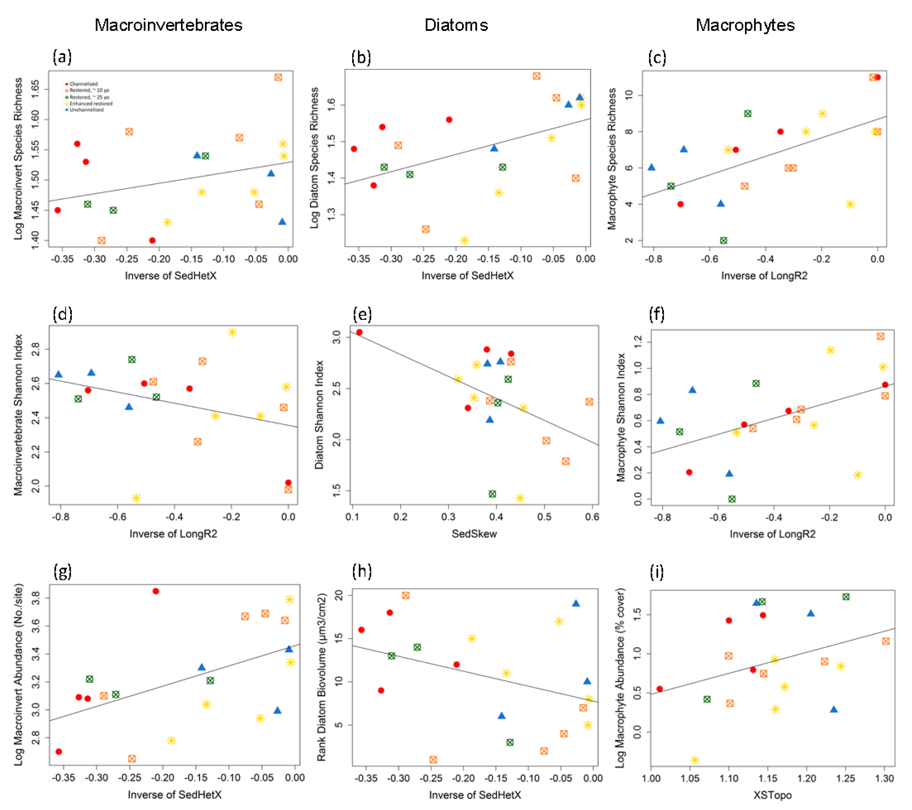
| Taxa | Metric | SedHetX | SedSD | SedSkew | LongR2 * | LongRuff † | XSTopo | DepthCV | BankRatio | WoodTot † | WoodBeav | WoodSaw | F | R2 | p | df |
| Macroinvertebrates | Species richness † | 0.45 | −0.48 | 0.47 | 3.47 | 0.28 | 0.041 | 3.16 | ||||||||
| Shannon index | −0.51 | 0.40 | 2.65 | 0.15 | 0.099 | 2.17 | ||||||||||
| Abundance † | 0.65 | −0.40 | 0.30 | 0.44 | 5.77 | 0.50 | 0.005 | 4.15 | ||||||||
| Diatoms | Species richness † | 0.48 | 5.33 | 0.19 | 0.033 | 1.18 | ||||||||||
| Shannon index | −0.46 | 4.78 | 0.21 | 0.042 | 1.18 | |||||||||||
| Biovolume ‡ | −0.71 | −0.44 | 0.57 | 4.69 | 0.37 | 0.016 | 3.16 | |||||||||
| Macrophytes | Species richness | −0.39 | −0.42 | 0.68 | 0.63 | 11.94 | 0.70 | <0.001 | 4.15 | |||||||
| Shannon index | 0.73 | 1.12 | 0.70 | 0.41 | −0.60 | 5.28 | 0.53 | 0.006 | 5.14 | |||||||
| Percent cover † | −0.46 | 0.56 | 3.45 | 0.20 | 0.055 | 2.17 | ||||||||||
| Diatoms | ||||
|---|---|---|---|---|
| Status | U | Chan | E | 10yo |
| Chan | 0.034 | |||
| E | 0.272 | 0.127 | ||
| 10yo | 0.292 | 0.060 | 0.924 | |
| 25yo | 0.400 | 0.055 | 0.053 | 0.094 |
© 2018 by the authors. Licensee MDPI, Basel, Switzerland. This article is an open access article distributed under the terms and conditions of the Creative Commons Attribution (CC BY) license (http://creativecommons.org/licenses/by/4.0/).
Share and Cite
Hasselquist, E.M.; Polvi, L.E.; Kahlert, M.; Nilsson, C.; Sandberg, L.; McKie, B.G. Contrasting Responses among Aquatic Organism Groups to Changes in Geomorphic Complexity Along a Gradient of Stream Habitat Restoration: Implications for Restoration Planning and Assessment. Water 2018, 10, 1465. https://doi.org/10.3390/w10101465
Hasselquist EM, Polvi LE, Kahlert M, Nilsson C, Sandberg L, McKie BG. Contrasting Responses among Aquatic Organism Groups to Changes in Geomorphic Complexity Along a Gradient of Stream Habitat Restoration: Implications for Restoration Planning and Assessment. Water. 2018; 10(10):1465. https://doi.org/10.3390/w10101465
Chicago/Turabian StyleHasselquist, Eliza Maher, Lina E. Polvi, Maria Kahlert, Christer Nilsson, Lisa Sandberg, and Brendan G. McKie. 2018. "Contrasting Responses among Aquatic Organism Groups to Changes in Geomorphic Complexity Along a Gradient of Stream Habitat Restoration: Implications for Restoration Planning and Assessment" Water 10, no. 10: 1465. https://doi.org/10.3390/w10101465