Article

Spatio-Temporal Characteristics of Tropospheric Ozone and Its Precursors in Guangxi, South China

1
State Key Laboratory of Remote Sensing Science, Institute of Remote Sensing and Digital Earth, Chinese Academy of Sciences, Beijing 100101, China
2
University of Chinese Academy of Sciences, Beijing 100049, China
3
China Centre for Resources Satellite Data and Application, Beijing 100830, China
*
Authors to whom correspondence should be addressed.
Atmosphere 2018, 9(9), 355; https://doi.org/10.3390/atmos9090355
Submission received: 4 August 2018 / Revised: 29 August 2018 / Accepted: 7 September 2018 / Published: 14 September 2018
(This article belongs to the Special Issue Air Quality in China: Past, Present and Future)

Abstract

:
The temporal and spatial distributions of tropospheric ozone and its precursors (NO2, CO, HCHO) are analyzed over Guangxi (GX) in South China. We used tropospheric column ozone (TCO) from the Ozone Monitoring Instrument (OMI) and Microwave Limb Sounder (MLS) onboard the Aura satellite (OMI/MLS), NO2 and HCHO from OMI and CO from the Measurements of Pollution in the Troposphere (MOPITT) instrument in the period 2005–2016. The TCO shows strong seasonality, with the highest value in spring and the lowest value observed in the monsoon season. The seasonal variation of HCHO is similar to that of TCO, while NO2 and CO show slightly different patterns with higher values in spring and winter compared to lower values in autumn and summer. The surface ozone, NO2 and CO observed by national air quality monitoring network sites are also compared with satellite-observed TCO, NO2 and CO, showing good agreement for NO2 and CO but a different seasonal pattern for ozone. Unlike TCO, surface ozone has the highest value in autumn and the lowest value in winter. To reveal the difference, the vertical profiles of ozone and CO from the measurement of ozone and water vapor by airbus in-service aircraft (MOZAIC) observations over South China are also examined. The seasonal averaged vertical profiles of ozone and CO show obvious enhancements at 2–6 km altitudes in spring. Furthermore, we investigate the dependence of TCO and surface ozone on meteorology and transport in detail along with the ECMWF reanalysis data, Tropical Rainfall Measuring Mission (TRMM) 3BV42 dataset, OMI ultraviolet index (UV index) dataset, MODIS Fire Radiative Power (FRP) and back trajectory. Our results show that the wind pattern at 800 hPa plays a significant role in determining the seasonality of TCO over GX, especially for the highest value in spring. Trajectory analysis, combined with MODIS FRP suggests that the air masses that passed through the biomass burning (BB) region of Southeast Asia (SEA) induced the enhancement of TCO and CO in the upper-middle troposphere in spring. However, the seasonal cycle of surface ozone is associated with wind patterns at 950 hPa, and the contribution of the photochemical effect is offset by the strong summer monsoon, which results in the maximum surface ozone concentration in post-monsoon September. The variations in the meteorological conditions at different levels and the influence of transport from SEA can account for the vertical distribution of ozone and CO. We conclude that the seasonal distribution of TCO results from the combined impact of meteorology and long-term transport.

1. Introduction

In recent years, with air pollution control, PM2.5 values have experienced a significant decline in China; however, ozone has replaced PM2.5 as the primary pollutant in South China during summertime, e.g., Guangdong province (http://kjs.mep.gov.cn/). Tropospheric ozone plays a key role in the regional and global atmosphere and climate systems. As the third most important greenhouse gas and one of the most important components of photochemical smog, tropospheric ozone originates from the stratosphere and troposphere exchange (STE) process and photochemical reactions involving its precursors, such as nitrogen dioxides (NOx = NO + NO2), volatile organic compounds (VOCs), CO and CH4 [1]. High concentrations of ozone have adverse effects on human health and ecosystem productivity near the surface layer [2,3,4,5,6,7,8]. Therefore, understanding and measuring ozone and its precursors has become more important, and tropospheric ozone has already been included as a routine monitoring component in the new air quality standard of 2013 (http://kjs.mep.gov.cn/).
Tropospheric column ozone (TCO) has different characteristics in different regions. Previous studies found that the seasonal variation of TCO is generally higher in summer and lower in winter, which is strongly due to photochemical activity [9]. However, measurement of TCO over East Asia, the western Pacific in Japan, Taiwan, Hong Kong and the Arabian sea show similar seasonal patterns with the maximum concentration occurring in spring [10,11,12]. In contrast, Sun et al. [13] observed a broad maximum in both spring and summer, with the maximum in June, and lower TCO values in autumn and winter in the western suburbs of Hefei city (the capital of Anhui Province) based on Fourier Transform Infrared Spectroscopy (FTIR) observations. There are many factors accounting for the observed seasonal characteristics. Vigouroux et al. [14] suggested that the most effective STE process during late winter and spring can account for the spring maximum in eight of the NDACC stations. Zhang and Chan found that lightning NOx emissions and/or stratospheric influences were responsible for the major events of high ozone observed in the UT/MT region over South China in spring [10,12]. Another important aspect that cannot be ignored is the transport of ozone [15], especially when the pollutants originate from anthropogenic or biomass burning (BB) sources [16,17,18,19]. BB introduces huge amounts of ozone precursors, i.e., NO2, CO, CH4, NMHCs and other VOCs, into the troposphere. Generally, the lifetime of these precursors is short; however the impact of BB on ozone is significant within and near the burning regions, with increases of ~10–25% in TCO relative to the average background concentrations [20]. Model studies showed that the pollutants emitted from South East Asian (SEA) BB in spring can be transported by the prevailing westerly wind to affect the air quality and chemistry downwind of southern China and the northwestern Pacific, and are most prominent at 700 hPa [21]. Meanwhile, intensive ground monitoring has been carried out in urban and rural areas at environmental protection stations over China, where daily surface ozone, NO2, CO and other near-ground data have been available since 2013. Wang et al. [22] found that ground-level ozone concentrations reached a minimum in winter and peaked in summer. However, some studies found that ground-level ozone concentrations peaked in autumn in the Pearl River Delta (PRD) region [23]. Previous studies proved that TCO seasonal variation changes linked closely to the study region location and revealed the inconsistency of seasonal cycles between ground-level ozone and TCO in some study areas.
Previous studies have also been conducted to understand variations of ozone and photochemical reactions between ozone and its precursors based on field measurements [24,25] and satellite measurements [1,26]. Ozone production can be controlled by either emissions of NOx or VOCs depending on the NOx-sensitive or VOC-sensitive photochemical regimes [27,28,29]. NO2 is released from both stationary (combustion of fuel) and mobile sources [30] and is usually enhanced in the boundary layer. NO2 exhibits the highest levels in winter and the lowest levels in summer/spring. There was a continuous increasing pattern from 2005 to 2012; thereafter, it showed a decreasing trend in China due to regulations [30,31]. In the absence of quantitative information on VOCs, HCHO was used as a proxy for VOCs, as it is a short-lived oxidation product of many VOCs [27]. HCHO columns are commonly found in large quantities over forested regions in the world, and a large fraction of HCHO columns were observed in industrial/urban regions in East Asia [31]. The seasonal variation shows a maximum in summertime in mid-latitude regions [32]. It is revealed that OMI HCHO shows an upward trend in northeastern China, resulting from the anthropogenic effect [33] and is negative in the PRD [31]. CO is also an ozone precursor, and determines the regional background values of the ozone level [1]; the relation of O3-CO has also been examined [34]. CO is produced from fuel combustion associated with transportation, industry and domestic heating. CO can be transported over long distances due to its long lifetime. Studies showed that the highest CO level is observed in late spring (April and May) and the lowest is observed in late fall (October and November) based on Measurements of Pollution in the Troposphere (MOPITT) CO columns, and that it shows an overall increasing trend in Beijing [35]. In contrast, CO reaches its maximum during winter and shows a broad minimum during the summer monsoon season, with a decreasing trend in India [36]. The changes in ozone precursors affect the photochemical conditions of ozone formation. To identify the ozone sensitivity to precursors, we need to understand their spatiotemporal characteristics from location to location. It is important to determine the ozone variation and to guide ozone control policy.
Guangxi (GX) is located in southern China and is also downwind of the SEA BB source area. It should be noted that GX is on the pathway which BB pollutants from SEA transporting to China must follow at 700 hPa. However, most previous studies paid less attention to this area or designated GX as part of South China, which may hide the seasonal characters for tropospheric ozone and its precursor. Furthermore, there are 50 national air quality monitoring sites in GX, but most of them are concentrated in urban areas and provide measurements of surface ozone, NO2, CO, PM2.5 and PM10 with limited spatial coverage. To obtain more knowledge about tropospheric ozone over GX, we analyze the spatial–temporal distribution patterns of tropospheric ozone and its precursors with satellite datasets (TCO data products form OMI/MLS, NO2, HCHO and UV index form OMI, CO form MOPITT), investigate the dependence of tropospheric ozone on meteorology and transport with ECMWF reanalysis data, MOZAIC aircraft observations, MODIS FRP, OMI UV index, TRMM rainfall and back trajectory analysis. In addition, surface ozone is also investigated.

2. Research Region and Datasets

2.1. Research Region

GX is located in southern China (104°26′ E–112°04′ E, 20°54′ N–26°24′ N), bordered by Yunnan to the west, Guizhou to the north, Hunan to the northeast, and Guangdong to the east and southeast. It is also bordered by Vietnam in the southwest and the Beibu Gulf in the south. GX covers a surface of 236,700 km2 and has a population of 48.85 million. The gross domestic product (GDP) was 2.039625 trillion RMB in 2017 (http://www.gxtj.gov.cn/). The topography is high in the northwest and low in the southeast. The relevant information is illustrated in Figure 1.

2.2. OMI/MLS TCO

The TCO dataset was retrieved from OMI/MLS onboard the Aura satellite based on the tropospheric ozone residual method. OMI is a nadir-viewing UV-VIS two-dimensional charged-coupled device (CCD) spectrometer. The instrument has a 114° field-of-view, producing a 2600 km wide swath that contains 60 pixels at a spatial resolution of up to 13 km × 24 km with near-daily global coverage. Its spectral range is 270–500 nm divided into three channels, UV-1 from 264 to 311 nm, UV-2 from 307 to 383 nm, and Vis from 349 to 504 nm, with spectral resolutions of 0.63, 0.42 and 0.63 nm, respectively, which is available for providing the total ozone column. MLS provides atmospheric parameters by observing the thermal emissions from the limb-viewing in broad spectral regions centered near 118, 190, 240, and 640 GHz, and 2.5 THz [37]. TCO is derived by subtracting the MLS stratospheric column from the OMI total column. Both the OMI-CCD and MLS measurements of the stratospheric ozone are averaged for the comparison over the Pacific (120° W–120° E) [38,39]. The MLS data are adjusted according to the observed differences and are then interpolated along the track and longitude respectively in two steps. OMI/MLS is able to provide daily global TOCs. The spatial resolution of the OMI/MLS TCO monthly mean product is 1.25° × 1°, with an uncertainty of five Dobson units (DU) and a mean offset of two DU [20].

2.3. OMI NO2 and HCHO

OMI allows for the retrieval of NO2 and HCHO based on the differential optical absorption spectroscopy (DOAS) algorithm, which first retrieves SCDs (slant column density) by spectral fitting, then converts the SCDs to VCDs (vertical column density) using air mass factors (AMFs). NO2 is retrieved in the 405–465 nm spectral region [40] and HCHO is retrieved in the 328.5–347 nm spectral region [32]. In this study, tropospheric monthly averaged NO2 vertical columns (derivation of OMI tropospheric NO2, DOMINO) are obtained from The Royal Netherlands Meteorological Institute (KNMI) and monthly averaged HCHO vertical columns are obtained from the Belgian Institute for Space Aeronomy (BIRA-IASB), both with spatial resolutions of 0.25° × 0.25°. The overall errors in the vertical tropospheric NO2 and HCHO column data are 10–40% and 25–41%, respectively [32,40].

2.4. MOPITT Total Column CO

Due to its two-month lifetime, CO is a tracer for biomass burning and the incomplete combustion of fossil fuels. Satellite observations of CO can clearly identify areas of intense burning [41] as well as urban areas [42]. In this study, the gridded dataset of monthly mean CO from MOPITT [43] with a spatial resolution of 1° × 1° was used. The MOPITT CO observations have been validated with aircraft in situ measurements and show good quality, with an average bias of less than 20 ppbv at all levels [44].

2.5. Ancillary Data

Fire radiative power (FRP): FRP is equivalent to the total radiative power of a fire, which is a measure of outgoing radiant heat from fire (in units of MW). The FRP retrieval for MODIS adopts the approach proposed by Wooster et al. [45], which is called the MIR (mid-infrared) radiance method [46]. Giglio et al. [46,47] proved that FRP can provide useful information about fire behavior. In this study, the MODIS monthly mean FRP product with a spatial resolution of 0.5° × 0.5° was used.
Hybrid single-particle Lagrangian integrated trajectory (HYSPLIT): HYSPLIT is a system for the computation of simple air parcel trajectories from the National Oceanic and Atmospheric Administration (NOAA) [48]. To investigate the forward and backward trajectory of the air mass, the web-based version of the HYSPLIT model was used for this study.
UV index (UVI): The OMI UV products (irradiances, erythemal doses and UVI) are developed jointly by the Finnish Meteorological Institute and NASA, generally with the cloud and aerosol corrections. The UVI is a dimensionless number that represents that the solar radiation reaching the surface can damage human skin when the sun is at its highest point in the sky, with ranges from 0 to 15. Comparisons with ground-based data reveal that the OMI UV product generally overestimates the surface UV index while the correlation is rather good and reliable [49,50,51]. Our study focuses on seasonal variation and pays more attention to relative changes than absolute values, so the dataset met the needs of this study. In this study, the UVI dataset from 2014 was used to evaluate the contribution of sunlight to ozone photochemicals.
MOZAIC: The MOZAIC program is currently known as the European In-service Aircraft for a Global Observing System (IAGOS) program [52], and has provided the vertical profiles of ozone, water vapor, carbon monoxide and other trace gases from aircraft take-off and landing since 1994 (https://www.iagos.org/). We used 121 profiles over South China (20° N–25° N, 105° E–115° E) in the period 2009–2012.
Wind field: The wind field from ECMWF in 2014 at different altitudes (950 hPa, 800 hPa and 650 hPa) was used in this study.
Rainfall: The TRMM satellite daily product, TRMM 3BV42 dataset (in units of mm/day), was used to measure precipitation, with a resolution of 0.25°, which was gauge-corrected by the Global Precipitation Climatology Center (GPCC) and the Climate Assessment and Monitoring System (CAMS). The correlation between the TRMM 3BV42 daily mean precipitation and the gauge station data over China is 0.7–0.83 during the period 2005–2013 according to a previous study [53].

3. Results and Discussion

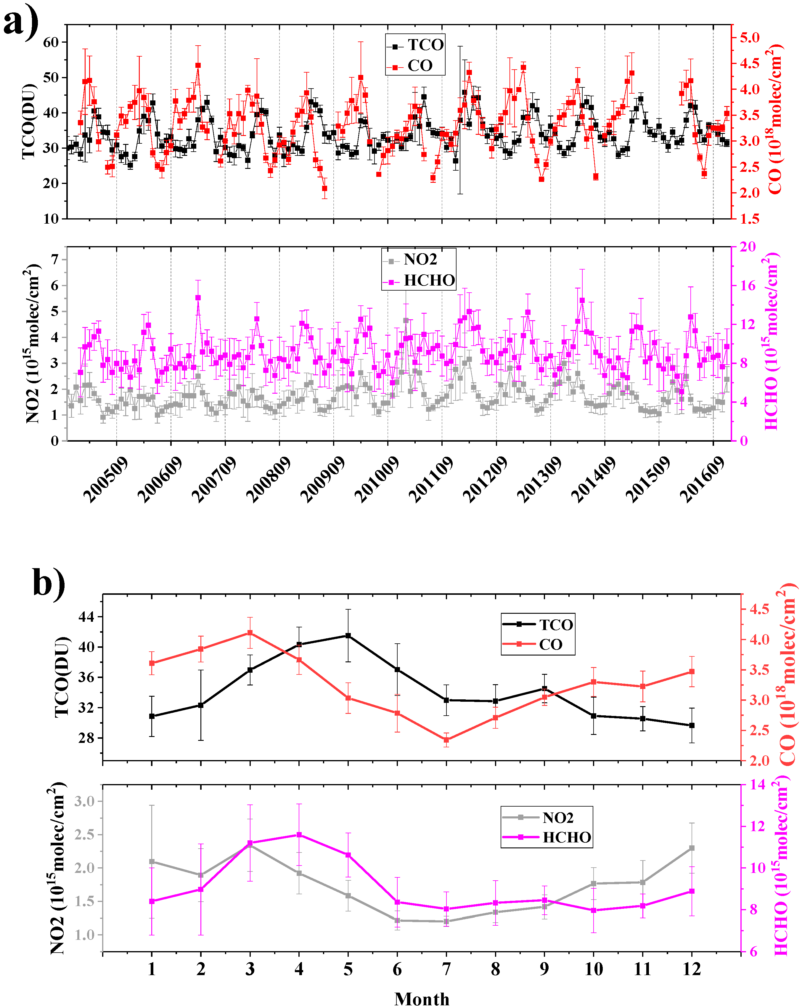
3.1. Spatial and Temporal Variations of TCO and Its Precursors

Figure 2 shows the time-series of monthly averaged and multiyear monthly averaged TCO, CO, NO2 and HCHO. Based on this we find that there was a slight increase during the period 2005–2016 for the TCO (Figure S2a) over GX. Figure 3a shows that the seasonal average TCO over GX is different from the typical seasonal variation in the North China and the Yangtze River Delta (YRD) region [23], where the highest ozone occurs from late May to July. The maximum TOC over GX was observed from April to May (~40 ± 3.3 DU in spring), the seasonal average value was lower in summer than in spring (~34.3 ± 3.4 DU), then decreased in autumn continuously (~32 ± 2.4 DU), and gradually declined to the minimum in winter (~30 ± 2.2 DU). However, it should be noted that the TCO did not decline continuously every month and exhibited a bimodal distribution in May and September (Figure 2b), showing a slight recovery in September. The spatial distribution of TCO is shown in Figure 4 (surrounded by white lines). The TCO was higher over eastern GX than over western GX in spring and in autumn (Figure 4a,c), was slightly higher over northern GX than over southern GX in summer (Figure 4b), while in winter (Figure 4d), the TCO was slightly higher over southern GX than over northern GX.
The time series of the monthly averaged NO2 VCDs in Figure 2a shows that there was a slight increase during the period 2005–2011, followed by a marked decrease from 2012 (Figure S2b) associated with the strict emissions regulations for reducing NO2 in China’s 12th Five-Year Plan [54]. The implementation of the SCR (selective reduction catalyst) system was promoted from 2013 and was fully completed in 2014 in key enterprises in GX, including coal-fired power enterprises, cement enterprises, and especially the sugar industry, which is the pillar industry in GX. It was reported by Guangxi Environmental Protection Bureau (http://www.gxepb.gov.cn/) that the NOx emissions fell 12.28% compared with 2013, which can account for the annual variations of NO2 VCDs observed here. Figure 3b shows that the NO2 VCD had seasonal average values of 1.88 ± 0.45 × 10¹⁵ molec/cm2, 1.26 ± 0.15 × 10¹⁵ molec/cm2, 1.68 ± 0.32 × 10¹⁵ molec/cm2 and 2.1 ± 0.60 × 10¹⁵ molec/cm2 for spring, summer, autumn and winter, respectively, which is consistent with the typical seasonal patterns in other regions [30,55]. Figure 5 shows that the highest value in winter is consistent with areas with a heavy industry base (such as Liuzhou) and densely populated areas (such as Nanning and the Beibu Gulf Economic Zone). However, it should be noted that the NO2 value over GX is obviously lower than the surrounding regions (such as PRD, central and eastern Hunan, western Guizhou), mainly due to the terrain and industrial development.
The multiyear monthly averaged HCHO columns in Figure 2b show that the maximum HCHO was observed from March–April, which is almost one month later than the maximum TCO. In addition, our results show that the HCHO columns were 8–11 times higher than the tropospheric NO2 VCDs over GX, and HCHO showed no significant decrease in pace with the NO2 decline since 2011 (Figure S2c shows that from 2005–2014, HCHO had a significant upward trend compared to the trend from 2005–2016), which was of great significance to the near-surface ozone photochemistry and the designation of ozone control policies over GX. Figure 3c shows that the seasonal average HCHO column had the maximum value in spring, 11.2 ± 1.58 × 10¹⁵ molec/cm2, compared with summer (8.21 ± 1.08 × 10¹⁵ molec/cm2), winter (8.75 ± 0.87 × 10¹⁵ molec/cm2) and autumn (8.20 ± 1.75 × 10¹⁵ molec/cm2). This result reveals a different seasonal pattern to the previous study regions, such as Beijing-Tianjin-Heibei (BTH) [56]. Figure 6 shows that the spatial distribution of HCHO over GX was similar to NO2 except in spring, with higher values over the central and eastern parts, while lower values were found over the western part. High HCHO values also appeared in PRD and Hanoi (the capital of Vietnam), which is in line with a previous study [33], indicating that anthropogenic activity has a significant impact on the spatial distribution of HCHO over this area. However, the HCHO columns were significantly higher in spring than other seasons, and especially had higher values in underdeveloped southwestern GX. This phenomenon cannot be explained by the dependence of the HCHO columns on temperature and anthropogenic activity, thus the anomalies of spring peaks of the HCHO columns were investigated in terms of meteorology and long-range transport, as described in Section 3.3.
The multiyear monthly averaged CO columns in Figure 2b show that the maximum was observed in March, which is consistent with the HCHO columns and with the maximum of TCO almost two months later. This temporal variation is in agreement with a previous study [11]. In addition, there was no obvious long-term trend for CO during the period 2005–2016 (Figure S2d), except that the global economic slowdown led to reductions in CO in 2009 [35]. Figure 3d shows that the seasonal averaged value of the CO columns was higher in spring (~3.6 ± 0.53 × 10¹⁸ molec/cm2) and winter (~3.65 ± 0.27 × 10¹⁸ molec/cm2), followed by autumn (3.23 ± 0.22 × 10¹⁸ molec/cm2), and the minimum was observed in summer (~2.6 ± 0.28 × 10¹⁸ molec/cm2), which reveals similar seasonal variations to NO2. It should be noted that there are noticeable spatial gradients of CO in spring compared with other seasons (Figure 7), with higher values in the west than in the east. In autumn and winter, higher CO columns are observed over eastern GX, while in summer, the northern values are higher than the southern values, although the overall CO columns are low. This distribution is further discussed in Section 3.3.

3.2. Comparison of Ground Observation and Satellite Observation

There are 50 national network sites in GX. The locations are shown in Figure 1b. Figure 8 presents the monthly mean ozone, and the NO2 and CO concentrations of all sites over GX compared with the satellite observation in 2016. The result shows the consistency of TCO and surface ozone is poor even though they both show a bimodal structure. The highest seasonal mean TCO occurred from April to May, with a secondary peak value in August, a month earlier than the multiyear monthly TCO shown in Figure 2b. This can be associated with the yearly TCO variation. In contrast, the surface ozone maximum was observed in September, with a secondary peak in May. For CO, there was a similar trend between the satellite and ground observations, except for April and July. The monthly variation characteristics of NO2 for the two data sets were almost consistent. According to the available detectable altitude range of satellite and ground observations, the discrepancy between the two data sets depends on the vertical distribution of the trace gases. We used the MOZAIC profile data over South China to examine the seasonal variation of the vertical distribution of ozone and CO. Figure 9 reveals that surface ozone is only a small part of TCO and the CO vertical profile is exponentially decreasing. Ozone and CO are significantly higher in spring than in summer at the 2–6 km altitude. It should be noted that we also observed elevated ozone in winter in the middle and upper troposphere, which was lower than in summer, but was noticeable. Above 6 km, the ozone concentration was highest in summer, followed by spring, autumn and winter, consistent with the typical seasonal pattern, and there was no significant seasonal difference for CO at this height. Below 1 km, the ozone concentration was slightly higher in autumn than in spring, and the summer concentration was lower than spring and higher than winter. For CO, the highest value was in winter, followed by spring, autumn and summer, which was consistent with the surface observation. The seasonal distribution features of CO showed no obvious discrepancy in spring and winter, which can be attributed to the initial seasonal distribution, which was higher in spring and winter. In conclusion, the enhancement at 2–6 km in spring can account for the discrepancy of the satellite and ground observations for ozone and CO. In this study, we also examined the potential factors that can account for the enhancement

3.3. Influence Factors

GX features a subtropical climate, the annual average temperature over approximately 65% of the province is above 20.0 °C, winter is shorter than summer, and seasonal differences of temperature are not significant over most of the area compared with north China. The monthly mean temperature of Naning (capital of GX) is shown in Figure S1 as an example, with the maximum in summer (33 °C), followed by autumn (28.7 °C), spring (26.2 °C) and winter (20.84 °C), which is consistent with the highest surface ozone observed at national network sites. The recoveries of TCO and HCHO in August or September can also be interpreted by temperature due to both of them depending on temperature. The precipitation over GX can also affect the spatiotemporal characteristics of TCO to some degree. Due to the alternation of winter and summer monsoon, the spatial–temporal distribution of precipitation over GX is uneven. The precipitation is concentrated in the north part in April, and in the southern part in July (the precipitation distribution over GX is shown in Figure 10). Precipitation plays a washout role for ozone and its precursors, which can partially account for the low TCO in summer [57]. However, the high values of TCO and HCHO in spring cannot be explained by the seasonal variations of temperature and precipitation.
In addition, since sufficient light is the necessary prerequisite for photochemical ozone production processes [27], the seasonal pattern of the UV index from OMI is illustrated in Figure 11. It can be seen that the solar radiation over GX and south China are similar to the mid-high latitude area, reaching the maximum in July. Therefore, it can be inferred that the sunlight condition is not the main contributor to the high values of TCO and HCHO in spring. To investigate the other potential factors, the influence of the wind field and transport are evaluated in the following section.

3.3.1. Influence of Wind Field

Generally, the East Asian Summer Monsoon (EASM) begins around mid-May and dissipates in August [58]. In summer, the monsoon comes from the ocean and the diffusion conditions are good. Some of the pollutants over South Asia are efficiently washed out of the atmosphere by the monsoon [59]. In autumn, wind comes from the land and the pollution may accumulate. GX is within the EASM region. The wind field influences the diffusion of ozone and its precursors in the atmosphere [57]. Figure 12 shows wind fields at 950 hpa in April, July, October and January. In January, the northeast wind prevails, and the wind speed is approximately 2 m/s, then the wind speed increased significantly (approximately 4 m/s) and the southeast wind blowing from the ocean prevailed in April. In July, the wind direction is predominately affected by the EASM, with an average wind speed of 3 m/s and the south wind prevailing. The monthly mean surface ozone values greatly depend on the wind field at this level (Figure 8), which is lower during the monsoon period than in the pre-monsoon and post-monsoon periods. In addition, the monsoon also impacts the spatial distribution of ozone and its precursors through wind and precipitation, which offset the increasing effect of local photochemical ozone production processes near the surface, resulting in the highest surface ozone concentration in September after the monsoon instead of in July. This result is in line with previous research [11,58] and proves that the monsoon is the main contributor to the seasonal behavior of ozone [60]. However, the maximum value of TCO in spring cannot be explained by the wind direction in April at this altitude, which is also inconsistent with the maximum concentration of surface ozone in September. The temporal inconsistency between TCO and surface ozone indicates that there must be differences at high altitude.
Figure 13 shows that at 800 hPa for each month, the wind speed increases significantly from 3 m/s in January to 9 m/s in April, though the southwest wind prevails in both months. Additionally, the wind speed in spring is stronger than that in other seasons and has a significant change in wind direction compared with 950 hPa, from southeast to southwest. This influence can be captured by the distribution of TCO and is in agreement with the results from Xu et al. [61]. Meanwhile, the temporal–spatial variation of CO and HCHO in spring can also be interpreted as the wind-driven effect at this altitude. This is evident for pollutants transported with the wind (see details in Section 3.3.2).

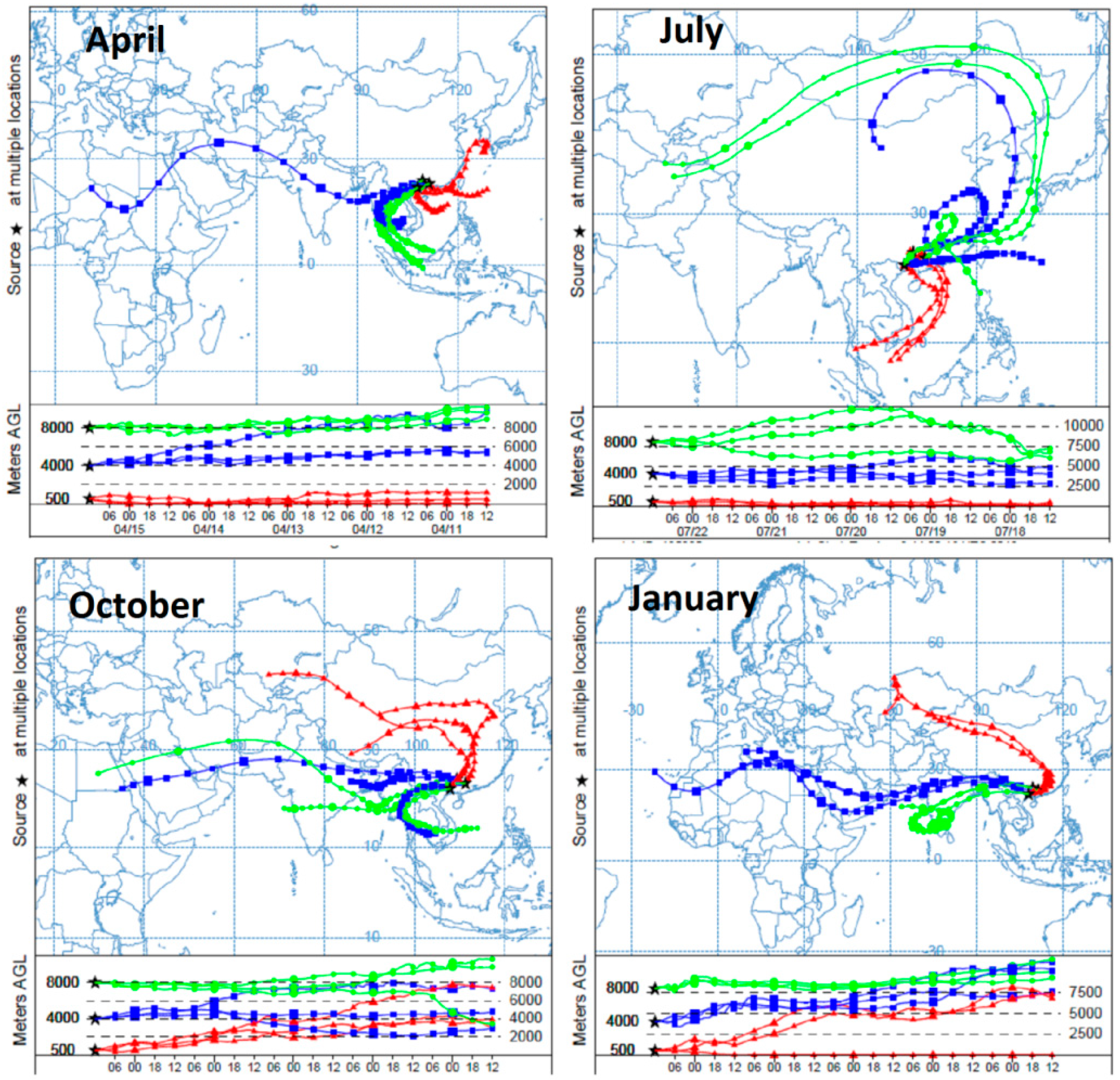
3.3.2. Long-Range Transport and Pollutant Accumulation

The five-day air mass back trajectories were obtained from the HYSPLIT model. Figure 14 shows an example of the HYSPLIT backward trajectory results for air masses over GX. Three points listed in Table 1 were selected for the backward trajectory analysis at altitudes of 500 m, 4 km and 8 km in January, April, July and October of 2014.
The results of the backward trajectory analysis show that air masses changed significantly according to altitude and season. In April, the air masses at an altitude of 500 m (red) were mainly from the southeast, and all back track air masses were lower than 2 km, while the air masses at 4 km (blue) and 8 km (green) altitudes mainly passed through Myanmar, Laos, Vietnam, and reached GX directly, which is consistent with the wind field at 800 hPa in April. It can be expected that the contaminants from the SEA BB origins brought by wind will affect TCO and its precursors over GX, especially in spring when SEA BB is most severe [62]. The spatial distribution of FRP is shown in Figure 15. In April (Figure 15a), the highest values of FRP were centered on Laos, affecting the chemical composition of the air masses flowing through this area directly. In July, the low troposphere air masses showed an obvious influence of the summer monsoon, which comes from the ocean; in the middle-upper troposphere the sources were identified as Mongolia and Afghanistan. In October, the air mass at the 500-m level was mainly affected by air flow from the northwest of China. At an altitude of 4 km, the air masses were mainly affected by westerly airflow, from eastern Africa, via the Arabian Gulf, India, Myanmar and Yunnan to GX. At the height of 8 km, it was predominantly influenced by the southwest airflow, from the Bay of Bengal to GX. The air masses in January had a similar pattern to October, where the middle troposphere air masses come from West Africa and those of the upper troposphere come from India.
Our results found that despite the different locations of the three points, they showed good consistency, except for the 500 m altitude in April. The sources were identified as SEA from 2 km to 8 km in April, which confirms the conclusion that the wind field at 800 hPa that passed through the BB region of SEA induces the enhancement of TCO and CO in spring. In wintertime, the ozone enhancements were most likely due to air masses transported along the subtropical jet from tropical and subtropical West Africa and South India.

4. Conclusions

We studied the spatial and temporal variations of TCO, NO2, CO and HCHO by analyzing data from the OMI/MLS and MOPITT instruments from 2005–2016 over GX. The 11-year monthly averaged TOC values had maximum values in spring and were in line with the seasonal pattern of the SEA BB. The spring average value was 40 DU, which is six DU higher than summer and 10 DU higher than winter. HCHO was consistent with the TCO seasonal pattern, with a maximum 11.2 × 10¹⁵ molec/cm2 in spring, and was 1.36 times higher than that in summer. In addition, CO and NO2 showed a similar seasonal cycle, where both were highest in winter and lowest in summer. The winter values were 1.4 and 1.7 times higher than in summer, respectively. Furthermore, we noticed a discrepancy between the satellite and ground observations for TCO and CO in spring over GX due to an obvious higher value at the altitude of 2–6 km of the vertical profile.
We examined the impact of meteorological conditions and long-range transport on the seasonal patterns of TCO and its precursors. We found that the highest TCO observed in spring was associated with the strong south-west wind at 800 hPa, which brings polluted air masses from SEA, where the level of BB is considerable. The conclusion was confirmed by the result of the backward trajectory analysis, which identified SEA as the source of middle and upper troposphere in spring. The joint effect of the wind field and transport was also captured by the vertical profile of ozone and CO from the MOZAIC data. However, the highest value of HCHO was also seen in spring, but we cannot provide a definitive conclusion regarding its source because of its short lifetime and because it is affected by biological sources and anthropogenic emissions. In summer, the air masses from the less polluted ocean result in the lowest value of NO2 and CO. Meanwhile, despite the best condition for the HCHO and O3 photochemical being in summer, the monsoon also has the biggest impact (with the largest amount of precipitation) during this period, which offset the increasing effect from the photochemicals. After the monsoon, there was a slight increase for TCO and HCHO over GX in autumn. These temporal characteristics observed from space can provide valuable information for ground measurements. Meanwhile, to explain the source of high HCHO in spring, the vertical observation of HCHO was needed over GX.
With respect to spatial distribution, NO2 was mainly concentrated in heavy areas. TCO was higher downwind, and CO and HCHO were both high in the west of GX in spring. We also found that the spatial distribution of HCHO was consistent with NO2 in autumn and winter, which revealed the impact of anthropogenic emissions on HCHO.

Supplementary Materials

The following are available online at https://www.mdpi.com/2073-4433/9/9/355/s1, Figure S1: Monthly averaged temperature over Naning (capital of GX) in the year 2017, Figure S2: Annual average and long trend of TCO and its precursors. The fitting lines are within 95% confidence intervals. (a) TCO(DU), (b) NO2(1015 molec/cm2), the red line represents the trend of 2005–2012, the black line represents the trend of 2012–2016, (c) HCHO (1015 molec/cm2), the red line represents the trend of 2005–2014, the black line represents the trend of 2005–2016, and (d) CO (1018 molec/cm2).

Author Contributions

Conceptualization, L.C. (Liangfu Cheng) and J.T.; Methodology, C.Y. and Y.W.; Validation, L.C. (Liangxiao Cheng) and H.W.; Formal Analysis, Y.W.; Resources, Z.W.; Data Curation, S.Z.; Writing-Original Draft Preparation, Y.W.; Revision, C.Y. and Y.S.

Funding

This research was funded by the National Key Research and Development Program of China (Grant No. 2017YFB0503901) and the National Natural Science Foundation of China (Grant No. 41771391 and 41501476).

Acknowledgments

We thank all the mission scientists and principal investigators who prepared for and provided the satellite data (OMI/MLS, MOPITT, and MODIS) used in this study. The authors are grateful to the ECMWF for the open-access reanalysis data. We are sincerely thankful for receiving the HYSPLIT free of charge. We thank Qiaolin Zeng for providing the TRMM data. We also thank Ziemke for providing the OMI/MLS TCO data.

Conflicts of Interest

The authors declare no conflict of interest.

References

  1. Choi, Y.; Souri, A.H. Seasonal behavior and long-term trends of tropospheric ozone, its precursors and chemical conditions over Iran: A view from space. Atmos. Environ. 2015, 106, 232–240. [Google Scholar] [CrossRef]
  2. Kondratyev, K.Y.; Varotsos, C.A. Global total ozone dynamics—Impact on surface solar ultraviolet radiation variability and ecosystems. Environ. Sci. Pollut. Res. 1996, 3, 205–209. [Google Scholar] [CrossRef] [PubMed]
  3. Amer Thoracic, S. What constitutes an adverse health effect of air pollution? Am. J. Respir. Crit. Care Med. 2000, 161, 665–673. [Google Scholar]
  4. Ashmore, M.R. Assessing the future global impacts of ozone on vegetation. Plant Cell Environ. 2005, 28, 949–964. [Google Scholar] [CrossRef] [Green Version]
  5. Fuhrer, J. Ozone risk for crops and pastures in present and future climates. Naturwissenschaften 2009, 96, 173–194. [Google Scholar] [CrossRef] [PubMed]
  6. Roux, E.; Hyvelin, J.M.; Savineau, J.P.; Marthan, R. Human isolated airway contraction—Interaction between air pollutants and passive sensitization. Am. J. Respir. Crit. Care Med. 1999, 160, 439–445. [Google Scholar] [CrossRef] [PubMed]
  7. Sun, J.; Koto, H.; Chung, K.F. Interaction of ozone and allergen challenges on bronchial responsiveness and inflammation in sensitised guinea pigs. Int. Arch. Allergy Immunol. 1997, 112, 191–195. [Google Scholar] [CrossRef] [PubMed]
  8. Monks, P.S.; Archibald, A.T.; Colette, A.; Cooper, O.; Coyle, M.; Derwent, R.; Fowler, D.; Granier, C.; Law, K.S.; Mills, G.E.; et al. Tropospheric ozone and its precursors from the urban to the global scale from air quality to short-lived climate forcer. Atmos. Chem. Phys. 2015, 15, 8889–8973. [Google Scholar] [CrossRef] [Green Version]
  9. Osterman, G.B.; Kulawik, S.S.; Worden, H.M.; Richards, N.A.D.; Fisher, B.M.; Eldering, A.; Shephard, M.W.; Froidevaux, L.; Labow, G.; Luo, M.; et al. Validation of Tropospheric Emission Spectrometer (TES) measurements of the total, stratospheric, and tropospheric column abundance of ozone. J. Geophys. Res. Atmos. 2008, 113. [Google Scholar] [CrossRef] [Green Version]
  10. Chan, C.Y.; Chan, L.Y.; Cui, H.; Zheng, X.D.; Zheng, Y.G.; Qin, Y.; Li, Y.S. Origin of the springtime tropospheric ozone maximum over east China at LinAn in 2001. Tellus 2010, 55, 982–992. [Google Scholar] [CrossRef]
  11. Jia, J.; Ladstätterweißenmayer, A.; Hou, X.; Rozanov, A.; Burrows, J.P. Tropospheric ozone maxima observed over the Arabian Sea during the pre-monsoon. Atmos. Chem. Phys. 2017, 17, 1–26. [Google Scholar] [CrossRef]
  12. Zhang, Y.Q.; Liu, H.Y.; Crawford, J.H.; Considine, D.B.; Chan, C.Y.; Oltmans, S.J.; Thouret, V. Distribution, variability and sources of tropospheric ozone over south China in spring: Intensive ozonesonde measurements at five locations and modeling analysis. J. Geophys. Res. Atmos. 2012, 117. [Google Scholar] [CrossRef] [Green Version]
  13. Sun, Y.; Liu, C.; Palm, M.; Vigouroux, C.; Hu, Q.; Tian, Y.; Wang, W.; Su, W.; Zhang, W.; Shan, C. Ozone seasonal evolution and photochemical production regime in polluted troposphere in eastern China derived from high resolution FTS observations. Atmos. Chem. Phys. Discuss. 2017. [Google Scholar] [CrossRef]
  14. Vigouroux, C.; De Maziere, M.; Demoulin, P.; Servais, C.; Hase, F.; Blumenstock, T.; Kramer, I.; Schneider, M.; Mellqvist, J.; Strandberg, A.; et al. Evaluation of tropospheric and stratospheric ozone trends over Western Europe from ground-based FTIR network observations. Atmos. Chem. Phys. 2008, 8, 6865–6886. [Google Scholar] [CrossRef] [Green Version]
  15. Zhou, D.; Ding, A.; Mao, H.; Fu, C.; Wang, T.; Chan, L.Y.; Ding, K.; Zhang, Y.; Liu, J.; Lu, A. Impacts of the East Asian monsoon on lower tropospheric ozone over coastal South China. Environ. Res. Lett. 2013, 8, 575–591. [Google Scholar] [CrossRef]
  16. Deng, X.; Tie, X.; Zhou, X.; Wu, D.; Zhong, L.; Tan, H.; Li, F.; Huang, X.; Bi, X.; Deng, T. Effects of Southeast Asia biomass burning on aerosols and ozone concentrations over the Pearl River Delta (PRD) region. Atmos. Environ. 2008, 42, 8493–8501. [Google Scholar] [CrossRef]
  17. Lin, Y.C.; Lin, C.Y.; Lin, P.H.; Engling, G.; Lin, Y.C.; Lan, Y.Y.; Chang, C.W.J.; Kuo, T.H.; Wei, T.H.; Ting, C.C. Influence of Southeast Asian biomass burning on ozone and carbon monoxide over subtropical Taiwan. Atmos. Environ. 2013, 64, 358–365. [Google Scholar] [CrossRef]
  18. Liu, H.; Chang, W.L.; Oltmans, S.J.; Chan, L.Y.; Harris, J.M. On springtime high ozone events in the lower troposphere from Southeast Asian biomass burning. Atmos. Environ. 1999, 33, 2403–2410. [Google Scholar] [CrossRef]
  19. Lin, M.; Holloway, T.; Carmichael, G.R.; Fiore, A.M. Quantifying pollution inflow and outflow over East Asia in spring with regional and global models. Atmos. Chem. Phys. 2010, 10, 4221–4239. [Google Scholar] [CrossRef]
  20. Ziemke, J.R.; Chandra, S.; Duncan, B.N.; Schoeberl, M.R.; Torres, O.; Damon, M.R.; Bhartia, P.K. Recent biomass burning in the tropics and related changes in tropospheric ozone. Geophys. Res. Lett. 2009, 36, 172–173. [Google Scholar] [CrossRef]
  21. Jian, Y.; Fu, T.M. Injection heights of springtime biomass-burning plumes over peninsular Southeast Asia and their impacts on long-range pollutant transport. Atmos. Chem. Phys. 2014, 14, 3977–3989. [Google Scholar] [CrossRef] [Green Version]
  22. Wang, W.N.; Cheng, T.H.; Gu, X.F.; Chen, H.; Guo, H.; Wang, Y.; Bao, F.W.; Shi, S.Y.; Xu, B.R.; Zuo, X. Assessing Spatial and Temporal Patterns of Observed Ground-level Ozone in China. Sci. Rep. 2017, 7, 3651. [Google Scholar] [CrossRef] [PubMed] [Green Version]
  23. Wang, T.; Xue, L.; Brimblecombe, P.; Lam, Y.F.; Li, L.; Zhang, L. Ozone pollution in China: A review of concentrations, meteorological influences, chemical precursors, and effects. Sci. Total. Environ. 2016, 575, 1582–1596. [Google Scholar] [CrossRef] [PubMed]
  24. Cheng, N.L.; Chen, Z.Y.; Sun, F.; Sun, R.W.; Dong, X.; Xie, X.M.; Xu, C.X. Ground ozone concentrations over Beijing from 2004 to 2015: Variation patterns, indicative precursors and effects of emission-reduction. Environ. Pollut. 2018, 237, 262–274. [Google Scholar] [CrossRef] [PubMed]
  25. Gao, W.; Tie, X.X.; Xu, J.M.; Huang, R.J.; Mao, X.Q.; Zhou, G.Q.; Chang, L.Y. Long-term trend of O-3 in a mega City (Shanghai), China: Characteristics, causes, and interactions with precursors. Sci. Total. Environ. 2017, 603, 425–433. [Google Scholar] [CrossRef] [PubMed]
  26. Varotsos, C.; Christodoulakis, J.; Tzanis, C.; Cracknell, A.P. Signature of tropospheric ozone and nitrogen dioxide from space: A case study for Athens, Greece. Atmos. Environ. 2014, 89, 721–730. [Google Scholar] [CrossRef] [Green Version]
  27. Duncan, B.N.; Yoshida, Y.; Olson, J.R.; Sillman, S.; Martin, R.V.; Lamsal, L.; Hu, Y.; Pickering, K.E.; Retscher, C.; Allen, D.J. Application of OMI observations to a space-based indicator of NOx and VOC controls on surface ozone formation. Atmos. Environ. 2010, 44, 2213–2223. [Google Scholar] [CrossRef] [Green Version]
  28. Choi, Y.; Kim, H.; Tong, D.; Lee, P. Summertime weekly cycles of observed and modeled NOx and O3 concentrations as a function of satellite-derived ozone production sensitivity and land use types over the Continental United States. Atmos. Chem. Phys. Discuss. 2012, 12, 6291–6307. [Google Scholar] [CrossRef] [Green Version]
  29. Martin, R.V.; Fiore, A.M.; Van Donkelaar, A. Space-based diagnosis of surface ozone sensitivity to anthropogenic emissions. Geophys. Res. Lett. 2004, 31, 337–357. [Google Scholar] [CrossRef]
  30. Zhang, L.; Lee, C.S.; Zhang, R.; Chen, L. Spatial and temporal evaluation of long term trend (2005–2014) of OMI retrieved NO2 and SO2 concentrations in Henan Province, China. Atmos. Environ. 2017, 154, 151–166. [Google Scholar] [CrossRef]
  31. Souri, A.H.; Choi, Y.; Jeon, W.; Woo, J.H.; Zhang, Q.; Kurokawa, J. Remote sensing evidence of decadal changes in major tropospheric ozone precursors over East Asia. J. Geophys. Res. Atmos. 2017, 122, 2474–2492. [Google Scholar] [CrossRef]
  32. De Smedt, I.; Stavrakou, T.; Hendrick, F.; Danckaert, T.; Vlemmix, T.; Pinardi, G.; Theys, N.; Lerot, C.; Gielen, C.; Vigouroux, C. Diurnal, seasonal and long-term variations of global formaldehyde columns inferred from combined OMI and GOME-2 observations. Atmos. Chem. Phys. 2015, 15, 12241–12300. [Google Scholar] [CrossRef]
  33. Smedt, I.D.; Stavrakou, T.; Müller, J.F.; Van der A, R.J.; Roozendael, M.V. Trend detection in satellite observations of formaldehyde tropospheric columns. Geophys. Res. Lett. 2010, 37, L18808. [Google Scholar] [CrossRef]
  34. Ding, A.J.; Wang, T.; Fu, C.B. Transport characteristics and origins of carbon monoxide and ozone in Hong Kong, South China. J. Geophys. Res. Atmos. 2013, 118, 9475–9488. [Google Scholar] [CrossRef] [Green Version]
  35. Li, L.; Liu, Y. Space-borne and ground observations of the characteristics of CO pollution in Beijing, 2000–2010. Atmos. Environ. 2011, 45, 2367–2372. [Google Scholar] [CrossRef]
  36. Girach, I.A.; Nair, P.R. Carbon monoxide over Indian region as observed by MOPITT. Atmos. Environ. 2014, 99, 599–609. [Google Scholar] [CrossRef]
  37. Waters, J.W.; Froidevaux, L.; Harwood, R.S.; Jarnot, R.F.; Pickett, H.M.; Read, W.G.; Siegel, P.H.; Cofield, R.E.; Filipiak, M.J.; Flower, D.A. The Earth observing system microwave limb sounder (EOS MLS) on the aura Satellite. IEEE Trans. Geosci. Remote. Sens. 2006, 44, 1075–1092. [Google Scholar] [CrossRef] [Green Version]
  38. Ziemke, J.R.; Chandra, S.; Labow, G.J.; Bhartia, P.K.; Froidevaux, L.; Witte, J.C. A global climatology of tropospheric and stratospheric ozone derived from Aura OMI and MLS measurements. Atmos. Chem. Phys. 2011, 11, 9237–9251. [Google Scholar] [CrossRef] [Green Version]
  39. Ziemke, J.R.; Chandra, S.; Duncan, B.N.; Froidevaux, L.; Bhartia, P.K.; Levelt, P.F.; Waters, J.W. Tropospheric ozone determined from aura OMI and MLS: Evaluation of measurements and comparison with the Global Modeling Initiative’s Chemical Transport Model. J. Geophys. Res. Atmos. 2006, 111. [Google Scholar] [CrossRef]
  40. Boersma, K.F.; Eskes, H.J.; Dirksen, R.J.; van der A, R.J. An improved tropospheric NO2 column retrieval algorithm for the Ozone Monitoring Instrument. Atmos. Meas. Tech. 2011, 4, 2329–2388. [Google Scholar] [CrossRef]
  41. Edwards, D.P.; Emmons, L.K.; Gille, J.C.; Chu, A.; Attié, J.L.; Giglio, L.; Wood, S.W.; Haywood, J.; Deeter, M.N.; Massie, S.T. Satellite-observed pollution from Southern Hemisphere biomass burning. J. Geophys. Res. Atmos. 2006, 111, 257–271. [Google Scholar] [CrossRef]
  42. Clerbaux, C.; Drummond, J.R.; Flaud, J.M.; Orphal, J. Using Thermal Infrared Absorption and Emission to Determine Trace Gases; Springer: Berlin/Heidelberg, Germany, 2011; pp. 123–151. [Google Scholar]
  43. Edwards, D.P.; Emmons, L.K.; Hauglustaine, D.A.; Chu, D.A.; Gille, J.C.; Kaufman, Y.J.; Pétron, G.; Yurganov, L.N.; Giglio, L.; Deeter, M.N. Observations of carbon monoxide and aerosols from the Terra satellite: Northern Hemisphere variability. J. Geophys. Res. Atmos. 2004, 109, 2561–2580. [Google Scholar] [CrossRef]
  44. Emmons, L.K.; Deeter, M.N.; Gille, J.C.; Edwards, D.P.; Attié, J.L.; Warner, J.; Ziskin, D.; Francis, G.; Khattatov, B.; Yudin, V. Validation of Measurements of Pollution in the Troposphere (MOPITT) CO retrievals with aircraft in situ profiles. J. Geophys. Res. Atmos. 2004, 109, 323–350. [Google Scholar] [CrossRef]
  45. Wooster, M.J.; Roberts, G.; Perry, G.L.W.; Kaufman, Y.J. Retrieval of biomass combustion rates and totals from fire radiative power observations: FRP derivation and calibration relationships between biomass consumption and fire radiative energy release. J. Geophys. Res. Atmos. 2005, 110. [Google Scholar] [CrossRef] [Green Version]
  46. Giglio, L.; Csiszar, I.; Justice, C.O. Global distribution and seasonality of active fires as observed with the Terra and Aqua Moderate Resolution Imaging Spectroradiometer (MODIS) sensors. J. Geophys. Res. Biogeosci. 2015, 111, 17–23. [Google Scholar]
  47. Giglio, L. Characterization of the tropical diurnal fire cycle using VIRS and MODIS observations. Remote. Sens. Environ. 2007, 108, 407–421. [Google Scholar] [CrossRef]
  48. Stein, A.F.; Draxler, R.R.; Rolph, G.D.; Stunder, B.J.B.; Cohen, M.D.; Ngan, F. NOAA’s HYSPLIT Atmospheric Transport and Dispersion Modeling System. Bull. Am. Meteorol. Soc. 2016, 96, 150504130527006. [Google Scholar] [CrossRef]
  49. Pitkänen, M.R.A.; Arola, A.; Lakkala, K.; Koskela, T.; Lindfors, A.V. Comparing OMI UV index to ground-based measurements at two Finnish sites with focus on cloud-free and overcast conditions. Atmos. Meas. Tech. Discuss. 2015, 8, 487–516. [Google Scholar] [CrossRef]
  50. Bernhard, G.; Arola, A.; Dahlback, A.; Fioletov, V.; Heikkilä, A.; Johnsen, B.; Koskela, T.; Lakkala, K.; Svendby, T.; Tamminen, J. Comparison of OMI UV observations with ground-based measurements at high northern latitudes. Atmos. Chem. Phys. 2015, 15, 8933–8981. [Google Scholar] [CrossRef]
  51. Zempila, M.M.; Fountoulakis, I.; Taylor, M.; Kazadzis, S.; Arola, A.; Koukouli, M.E.; Bais, A.; Meleti, C.; Balis, D. Validation of OMI erythemal doses with multi-sensor ground-based measurements in Thessaloniki, Greece. Atmos. Environ. 2018, 183, 106–121. [Google Scholar] [CrossRef]
  52. Nédélec, P.; Blot, R.; Boulanger, D.; Athier, G.; Cousin, J.M.; Gautron, B.; Petzold, A.; Volzthomas, A.; Thouret, V. Instrumentation on commercial aircraft for monitoring the atmospheric composition on a global scale: The IAGOS system, technical overview of ozone and carbon monoxide measurements. Tellus Ser. B Chem. Phys. Meteorol. 2015, 67, 6. [Google Scholar] [CrossRef] [Green Version]
  53. Zeng, Q.; Wang, Y.; Chen, L.; Wang, Z.; Zhu, H.; Li, B. Inter-Comparison and Evaluation of Remote Sensing Precipitation Products over China from 2005 to 2013. Remote. Sens. 2018, 10, 168. [Google Scholar] [CrossRef]
  54. Jin, Y.; Andersson, H.; Zhang, S. Air Pollution Control Policies in China: A Retrospective and Prospects. Int. J. Environ. Res. Public Health 2016, 13, 1219. [Google Scholar] [CrossRef] [PubMed]
  55. Cheng, M.M.; Jiang, H.; Guo, Z. Evaluation of long-term tropospheric NO2 columns and the effect of different ecosystem in Yangtze River Delta. Procedia Environ. Sci. 2012, 13, 1045–1056. [Google Scholar] [CrossRef]
  56. Zhu, S.Y.; Li, X.Y.; Yu, C.; Wang, H.M.; Wang, Y.P.; Miao, J. Spatiotemporal Variations in Satellite-Based Formaldehyde (HCHO) in the Beijing-Tianjin-Hebei Region in China from 2005 to 2015. Atmosphere 2018, 9, 24. [Google Scholar] [CrossRef]
  57. David, L.M.; Nair, P.R. Tropospheric column O3 and NO2 over the Indian region observed by Ozone Monitoring Instrument (OMI): Seasonal changes and long-term trends. Atmos. Environ. 2013, 65, 25–39. [Google Scholar] [CrossRef]
  58. Li, S.; Wang, T.J.; Huang, X.; Pu, X.; Li, M.M.; Chen, P.L.; Yang, X.Q.; Wang, M.H. Impact of East Asian Summer Monsoon on Surface Ozone Pattern in China. J. Geophys. Res. Atmos. 2018, 123, 1401–1411. [Google Scholar] [CrossRef]
  59. Lelieveld, J.; Bourtsoukidis, E.; Bruhl, C.; Fischer, H.; Fuchs, H.; Harder, H.; Hofzumahaus, A.; Holland, F.; Marno, D.; Neumaier, M.; et al. The South Asian monsoon-pollution pump and purifier. Science 2018, 361, 270–273. [Google Scholar] [CrossRef] [PubMed]
  60. Safieddine, S.; Boynard, A.; Hao, N.; Huang, F.; Wang, L.; Ji, D.; Barret, B.; Ghude, S.D.; Coheur, P.F.; Hurtmans, D. Tropospheric Ozone Variability during the East Asian Summer Monsoon as Observed by Satellite (IASI), Aircraft (MOZAIC) and Ground Stations. Atmos. Chem. Phys. 2015, 15, 31925–31950. [Google Scholar] [CrossRef]
  61. Xu, J.; Ma, J.Z.; Zhang, X.L.; Xu, X.B. Measurements of ozone and its precursors in Beijing during summertime: Impact of urban plumes on ozone pollution in downwind rural areas. Atmos. Chem. Phys. 2011, 11, 12241–12252. [Google Scholar] [CrossRef] [Green Version]
  62. Kondo, Y.; Morino, Y.; Takegawa, N.; Koike, M.; Kita, K.; Miyazaki, Y.; Sachse, G.W.; Vay, S.A.; Avery, M.A.; Flocke, F. Impacts of biomass burning in Southeast Asia on ozone and reactive nitrogen over the western Pacific in spring. J. Geophys. Res. Atmos. 2004, 109, 2890–2898. [Google Scholar] [CrossRef]
Figure 1. Locations of the study areas: (a) The location of Guangxi in China; (b) Distribution of national network sites in GX.
Atmosphere 09 00355 g001
Figure 2. (a) Time-series of monthly averaged TCO, CO, NO2 and HCHO (raw data); (b) Multiyear monthly averaged TCO, CO, NO2 and HCHO (based on the raw data present in (a)). Vertical bars indicate one standard deviation.
Atmosphere 09 00355 g002
Figure 3. The seasonal boxplots of TCO (a), NO2 (b), HCHO (c) and CO (d) (based on the 95% confidence interval of raw data present in Figure 2a).
Atmosphere 09 00355 g003
Figure 4. Seasonal-averaged OMI/MLS TCO for 2005–2016. (a) MAM; (b) JJA; (c) SON; (d) DJF.
Atmosphere 09 00355 g004
Figure 5. Seasonal-averaged OMI NO2 VCDs for 2005–2016. (a) MAM; (b) JJA; (c) SON; (d) DJF.
Atmosphere 09 00355 g005
Figure 6. Seasonal-averaged OMI HCHO columns for 2005–2016. (a) MAM; (b) JJA; (c) SON; (d) DJF.
Atmosphere 09 00355 g006
Figure 7. Seasonal-averaged MOPITT CO columns during the daytime for 2005–2016. (a) MAM; (b) JJA; (c) SON; (d) DJF.
Atmosphere 09 00355 g007
Figure 8. Monthly averaged satellite observed TCO (O3_S), CO (CO_S) and NO2 (NO2_S) and ground observed surfaced ozone (O3_G), CO (CO_G) and NO2 (NO2_G) in 2016.
Atmosphere 09 00355 g008
Figure 9. Seasonal-averaged profiles of ozone and CO from MOZAIC (20° N–25° N, 105° E–115° E). Horizontal bars indicate one standard deviation across multiple profiles.
Atmosphere 09 00355 g009
Figure 10. Rainfall distribution in 2014 based on TRMM (a) April; (b) July; (c) October; (d) January.
Atmosphere 09 00355 g010
Figure 11. UV index distribution in 2014 based on OMI. (a) April; (b) July; (c) October; (d) January.
Atmosphere 09 00355 g011
Figure 12. Monthly winds at 950 hPa in 2014 based on ECMWF. (a) April; (b) July; (c) October; (d) January. (The red line indicates the GX border).
Atmosphere 09 00355 g012
Figure 13. Monthly winds at 800 hPa in 2014 based on ECMWF. (a) April; (b) July; (c) October; (d) January.
Atmosphere 09 00355 g013
Figure 14. HYSPLIT model results with 120 h backward trajectory for air masses over GX with source locations at 500 m, 4000 m and 8000 m altitudes in April, July, October and January 2014.
Atmosphere 09 00355 g014
Figure 15. Spatial distribution of Fire radiative power in 2014 based on MODIS. (a) April; (b) July; (c) October; (d) January.
Atmosphere 09 00355 g015
Table 1. Information about the three points for the backward trajectory analysis.
NameLocationRepresentative Type
Liuzhou city109°40′ E, 24°33′ NIndustrial base
Chongzuo city107°92′ E, 22°42′ NAdjacent to Vietnam
Wuzhou city108°35′ E, 21°78′ NAn inland city

