Article

How Sea Fog Influences Inland Visibility on the Southern China Coast

1
College of Oceanic and Atmospheric Sciences, Ocean University of China, Qingdao 266100, China
2
Institute of Tropical and Marine Meteorology, China Meteorological Administration, Guangzhou 510080, China
*
Author to whom correspondence should be addressed.
Atmosphere 2018, 9(9), 344; https://doi.org/10.3390/atmos9090344
Submission received: 1 August 2018 / Revised: 29 August 2018 / Accepted: 29 August 2018 / Published: 3 September 2018
(This article belongs to the Special Issue Storms, Jets and Other Meteorological Phenomena in Coastal Seas)

Abstract

:
Sea fog can lead to inland fog on the southern China coast, affecting visibility on land. To better understand how such fog influences inland visibility, we observed two sea-fog cases at three sites (over sea, at coast, and inland) and analyzed the results here. Our analysis suggests four factors may be key: (1) The synoptic pattern is the decisive factor determining whether fog forms inland. First, sea fog and low clouds form when the synoptic pattern involves warm, moist air moving from a warmer sea-surface temperature (SST) region to a colder SST region near the coast. Then, inland fog tends to occur under this low-cloud background with relatively large horizontal-vapor transport. A greater horizontal-vapor transport results in denser fog with higher liquid-water content. Conversely, a strong horizontal advection of temperature with less horizontal-vapor transport can hinder inland-fog formation. (2) Local cooling (including ground radiative cooling) helps promote inland fog formation. (3) Fog formation requires low wind speed and small turbulent kinetic energy (TKE). The small TKE helps the vapor accumulate close to the surface and maintain the local cooling effect. (4) Fog formation is promoted by having the energy flux downward at night with the land surface cooling the atmosphere as well as having lower soil temperature and higher soil humidity.

1. Introduction

Sea fog severely influences marine navigation as well as activities in harbors and coastal airports around the world [1,2,3,4]. This fog can drift inland. For example, Lamb (1943) [5] found that the sea fog (haar) of Scotland can move inland during the day if insolation is weak. He also noted that this inland fog tends to clear during the day and thicken at night. Leipper (1994) [6] found that coastal fog on the U.S. West Coast forms with an unusually strong inversion below 400 m, but stratus forms, instead, if the inversion is relatively weak and the inversion height is above 400 m. Thus, a strong inversion inland is needed for sea fog to persist inland. More recently, Koračin et al. (2005) [7] found the cloud–fog transition to be determined by a combination of synoptic and boundary-layer processes, with the dissipation of sea fog being a consequence of a complex interplay between advection, synoptic evolution, and development of local circulations.
Compared to sea-fog formation, inland-fog formation involves different physical processes. Petterssen (1939) [8], and later Jiusto (1981) [9], argued that the three most important formation processes are the cooling of air, the addition of water vapor, and the mixing of moist air parcels of different temperatures. Duynkerke (1991) [10] describes the importance of more specific processes; in particular, the cooling of moist air by radiation flux, the vertical mixing of heat and moisture, horizontal and vertical wind, heat and moisture transport in soil, advection, and topographic effects. Bergot and Guedalia (1994) [11] argued that the local atmospheric cooling is critical for fog to form at night. Duynkerke (1999) [12] examined the effect of long-wave radiation on the structure of the clear, stable boundary layer as well as the relationship between radiative cooling near the surface and the top of the boundary layer together with its impact on the heat-flux profile. He thought it is necessary to further quantify the relative importance of radiative cooling and turbulence for the formation of fog. Zhou and Ferrier (2008) [13] pointed out that the small turbulence intensity inside a fog will help it persist. Steeneveld et al. (2010) [14] found the observed long-wave radiative heating to be minimal at the evening transition, and they argued that the total radiative-heating rate appears to be controlled by the upward long-wave flux divergence at night. Sun et al. (2017) [15] analyzed two sea-fog cases over the Yellow Sea to determine their influence on the coastal area. They argued that large-scale transport and boundary-layer structure are critical. However, their work lacks micrometeorological observations, and thus cannot determine the small-scale aspects of the mechanism. Overall, the mechanism of the sea-fog influence on inland visibility needs to be better understood.
On the southern China coast, inland fog associated with sea fog is difficult to predict during the sea-fog season (from January to May [16]). In some cases, extensive fog exists inland during a sea-fog event, but not always. Moreover, sometimes the inland fog that occurs with sea fog is patchy, adding to the forecast difficulty [17,18]. To address coastal-weather issues such as this, the Institute of Tropical and Marine Meteorology (ITMM) established the Marine Meteorological Science Experiment Base (MMSEB) at Bohe, Maoming in 2007. Then, in 2008, the Integrated Observation Platform for Marine Meteorology (IOPMM) was set up over sea and began acquiring many observation datasets of sea fog [19]. Based on these data, ITMM investigated the formation mechanism, the microphysics structure, and the characteristics of the boundary layer during sea fog [20,21,22]. Here, we use observations of two sea-fog cases at three sites (over sea, at coast, and inland) to better understand how sea fog influences inland visibility on the southern China coast.

2. Observational Sites and Data

2.1. Observational Sites and Data

We used observational data from three sites: site A on the coast, site B over sea, and site C inland. See Figure 1 for their locations. These three sites are the same as those in our previous study [23]. Site A is the MMSEB and operated by the Institute of Tropical Marine and Meteorology (ITMM) (Figure 1a). Site B is the IOPMM. Site C is the Dianbai National Climate Observatory (DNCO) (Figure 1b). Figure 1b shows the distances between the three sites and to the coastal line.
The land–atmosphere and air-sea surface data come from instruments mounted at three sites. We collect data on two sea-fog cases in March 2017. The observation system over land and sea (i.e., sites C, B) both include an instrument tower equipped with gradient- and flux-observation systems (Figure 1c,d), whereas we released a GPS sonde at coast (site A). Inland, the iron tower is 10 m high, with instruments to measure fluxes at the top. Other instruments include an automatic meteorological station, radiometers, and instruments to measure ground temperature and humidity, skin temperature, and soil heat flux (Figure 1c,d; Table 1).
The sea site lies above ~15 m of water, and the regular triangle platform is about 11 m above sea level. The instruments, listed in Table 1, and observational procedures are the same as before [23], except the present study does not have sea-temperature measurements. See Reference [23] for more details about the IOPMM.
During each sea-fog period, we launched a GPS Vaisala RS-92 sonde about every 3 h from the coastal site. The first period, hereafter case 1, ran from 0900 LST Mar 10 to 0500 LST Mar 11, the second, case 2, from 1200 LST Mar 30 to 1100 LST Mar 31. In total, 12 GPS sondes were released during the two events. As in our previous study [23], processing of the GPS sonde data and calculation of the equivalent potential temperature ( θ e ) follows that in Reference [24].
We used ultrasonic anemometers and infrared CO2/H2O analyzers at the inland and oversea sites. We calculated the turbulence flux and turbulent kinetic energy (TKE) with EddyPro 6.0 software over time intervals of 30 min. The software uses the Foken et al. method [25] to run quality-control tests of the fluxes as shown in Table 2. See our previous study [23] for more details.

2.2. Satellite Data

We used the Himawari-8 satellite data to determine fog and cloud extent near the southern China coast. Himawari-8 is the 8th Himawari geostationary weather satellite operated by the Japan Meteorological Agency, entering operational service on 7 July 2015. Himawari-8 provides 16-channel imagery, including visible- and infrared-band scanning of the Asia-Pacific region [26]. We used hourly imagery with 0.05° horizontal resolution, which was freely obtained from Kochi University (http://weather.is.kochi-u.ac.jp/wiki/archive).
Daytime-sea-fog retrieval mainly includes (1) cloud and clear detection based on the visible channel; (2) sea-fog and other cloud detection based on both the temperature difference between the cloud top and sea surface [27], as well as the standard deviation in the thermal infrared channel [28]; and (3) night-time sea-fog detection that mainly relies on the dual-channel difference test [28,29].

2.3. Other Data

The sea-surface temperature data come from the real-time global (RTG) data from the National Center for Environmental Prediction (NCEP) [30] and the NCEP Global Analysis on 1° × 1° grid-spacing datasets from the National Center for Environmental Prediction/National Weather Service/NOAA/U.S. Department of Commerce (2000). Backward-airflow trajectories come from our use of the HYSPLIT trajectory model and reanalysis data from the Global Data Assimilation System (GDAS) [31]. See Huang et al. [22] for more details.

3. Synoptic Backgrounds and Influence on Inland Visibility of the Two Cases

Both sea-fog cases were warm-advection fog. Warm-advection fog is the most common sea fog on the southern China coast. With this fog, the surface-air temperature (SAT) usually exceeds the sea-surface temperature (SST). Warm-advection fog forms by the lowering of an existing cloud base, and its growth is mainly driven by the advection of warm moist air [22]. We examine these cases to better understand how sea fog influences inland visibility. For the analysis periods of both sea fog cases at the three sites, see Table 3.
In case 1, at 1400 LST 10 March, which was before the fog formed over sea, mainly a southern wind prevailed, transporting warm, moist air to the observational site. However, a dry, strong northeast wind dominated at the Taiwan Strait, preventing fog formation there (Figure 2a). By 0200 LST 11 March, sea fog had formed, the wind was southeastern and nearly along the isobars, but was still bringing warm, moist air to the observational site. Meanwhile, the dry northeast wind at the Taiwan Strait remained strong (Figure 2c). At 1400 LST 11 March, this dry northeast wind extended over the north of the South China Sea, dissipating the fog (Figure 2e).
In case 2, the synoptic pattern differed because the sea fog encountered a cold front. First, at 1400 LST 30 March, a southeastern wind brought warm, moist air to the southern China coast, causing fog to form over the sea (Figure 2b). Then, at 0200 LST 31 March, a cold front appeared at the south side of the Nanling Mountains (110–116° E, 24–26.5° N). At the same time, the warm, moist wind kept on blowing towards the observational site, further developing the sea fog (Figure 2d). Later, at 1400 LST 31 March, the cold front moved across the coastline, resulting in the dissipation of the sea fog (Figure 2f).
In both cases, coastal visibility was hazardous near coastal site A (Figure 3a,b). The retrieved satellite data indicate more extensive sea fog near site A in case 1 than in case 2 (Figure 3c–f). Case 1 also appeared to have more inland fog than case 2. At the inland site C (DNCO), fog occured in case 1 with visibility of 0.1 km, but not in case 2 (Figure 4a,b). The aim was to determine the cause of this difference.
Consider the relative humidities (RH). In case 1, fog was reported inland when the visibility was about 1.0 km and RH = 96.5%. So, we used RH = 96.5% as the RH criterion for inland fog. However, the sensors at the oversea site experienced greater aging effects (due to greater sea-salt erosion and longer time before maintenance or replacement), and, by the same procedure, we found that RH = 95% gave the same criterion for fog over the sea. By this measure, the fog over the sea occurred from 1600 LST 10 March to 0900 LST 11 March, and from 2300 LST 10 March to 0800 LST 11 March at inland in case 1 (Figure 5a). Before the fog occurred, the inland region was overcast. An observer at site C noted dense fog at 0200 and 0500 LST 11 March at inland (Table 4). Applying the same criteria to case 2, we determined that fog occurred from 0430 LST 30 March to 1130 LST 31 March over sea, while no fog occurred inland (Figure 5b). The RH briefly exceeded 96.5% after 0800 LST 31 March, but it was due to a small rain. We will later discuss this event. The weather during case 2 was also cloudy inland, with a light fog at night. However, no fog formed and the lowest visibility was 3.2 km at 0500 LST 31 March (Table 4).

4. Advection and Boundary-Layer Characteristics

In fog season, warm, moist air that advects from the warmer SST area south of the 23 °C isotherm and mixes with air in the colder SST region near the coast always results in fog and low clouds. To examine these processes, we calculated the 48 h backward trajectories of airflow to the inland site for both cases at 20 m, 100 m, and 300 m heights. The surface air in both cases came from the warmer SST areas, but different locations. For case 1, Figure 6a shows the air origin to be the northern area of the South China Sea, and, for case 2, Figure 6b shows the origin to be the Bashi Channel (Luzon Strait). The figure also shows that the colder SST region around the southern China coast in case 1 is larger than that in case 2, which helps to create more extensive fog in case 1.
We calculated the horizontal advection of temperature to show the warm advection characteristics using the NCEP Global Analysis on 1° × 1° grid-spacing datasets. Results in Figure 7 show that for case 1, the warm advection moved mostly towards the Beibu Gulf and the west Guangdong area, whereas for case 2, it spread over nearly the whole southern China coast. Surprisingly, given the observed visibilities, the warm advection moved into the inland area more in case 2 than in case 1. To help understand this finding, we examined the average values of three 6 h time periods: for case 1, starting at 2000 LST 10 March, 0200 LST 11 March, and 0800 LST 11 March; for case 2, from 2000 LST 30 March, 0200 LST 31 March, and 0800 LST 31 March. The region is 20°–21° N, 111°–112° E. For case 1, the values are 0.31 × 10⁻⁴ K s−1 at 1000 hPa and 0.23 × 10⁻⁴ K s−1 at 975 hPa. For case 2, the values are 0.21 × 10⁻⁴ K s−1 at 1000 hPa and 0.32 × 10⁻⁴ K s−1 at 975 hPa (Figure 7a–d). To calculate the horizontal advection of vapor, we used the same datasets. The resulting vapor advection in Figure 8 has a similar pattern as the temperature advection. However, the average values over the same time and region give, for case 1, the values 0.35 × 10⁻⁴ g kg−1 s−1 at 1000 hPa and 0.22 × 10⁻⁴ g kg−1 s−1 at 975 hPa, which are much larger than the case 2 values of 0.15 × 10⁻⁴ g kg−1 s−1 at 1000 hPa and 0.07 × 10⁻⁴ g kg−1 s−1 at 975 hPa. Thus, there is more vapor advection to site C in case 1 than in case 2.
The GPS sondes at the coast site (MMSEB) depicted the boundary-layer structures during both fog cases. The data are plotted in Figure 9. The wind vectors of both cases mostly showed a consistent, but relatively weak, southern or eastern wind at the lower level, and a stronger western wind at the upper level. Both cases showed a warm layer below about 400 m. Considering the humidity, we used RH = 98% to define the cloud edge (appropriate for GPS sonde data [21]). As such, the figure shows that both fog cases formed by the lowering of the cloud base. The RH in case 2 also shows the fog transitioning back into stratus again. Case 1 had the observed highest fog top of about 1310 m at 0500 LST 11 March, whereas case 2 reached the slightly lower top of 910 m at 0200 LST 31 March.
Consider now the fog structures at the time of highest fog top. From the potential equivalent temperatures (Figure 10), we found that the thermal-turbulence interface (where θ e z = 0 ) occurred at a height of about 290 m in case 1 and about 170 m in case 2. In both cases, the profiles of potential equivalent temperature above the thermal-turbulence interface are nearly constant, meaning that the layers were well-mixed. This result agrees with that reported in References [21,22]. Overall, the boundary-layer structure in case 1 shows stronger warm and moist advection, which is more suitable for the development of sea fog, and also resulted in a higher fog top than that in case 2 (Figure 10a,b).

5. Differences of Meteorological Variables

We now focus on the main meteorological variables and turbulent kinetic energies, considering differences between those at sea and inland.
In case 1, the average temperature at the inland site was hotter than that at the oversea site (by 2.5 °C from 0800 to 2000 LST 10 March), with a maximum difference around 1400 on 10 March 2017 (Figure 11a). Later, from about 1500 that day, the inland site cooled by about 3.3 °C until the inland fog formed at 2300 LST 10 March. This cooling was due to cold advection to the inland site.
For case 2, the average inland temperature was also hotter than that over sea (by 3.3 °C from 0800 to 2000 LST 30 March), with a maximum difference during daytime at about 1600 LST 30 March. However, the cooling effect was not as strong in this case, with temperature dropping slowly by only 2.4 °C by the next morning at 0800 LST 31 March (Figure 11b). As with case 1, the cooling effect was consistent with the horizontal advection of temperature shown in Figure 7. But in this case, warm advection prevailed all the time at the inland site, hindering the radiative-cooling effect. In general, this case also has much less temperature variation over sea than that in case 1.
Consider now the wind prior and during the sea fog in case 1. Figure 11c shows that before the fog formed, the wind direction changed from northeast to southeast at about 1500 LST 10 March over sea, with fog forming one hour later. After the fog formed, the wind direction returned to northeast, but was steadier in direction. Meanwhile, the wind speed was low before the fog forms, but gradually increased after the fog forms.
Compared to the sea-fog event, the inland fog in case 1 showed a different wind pattern. The wind speed became very low when the fog first formed, making the wind direction erratic (though mainly southeast). Later, the wind speed increases by about 2 m s−1, and the wind direction changed from northeast to east (Figure 11c).
For case 2, the wind direction was relatively steady over sea and at inland, being east over sea and southeast at inland. The wind speeds at both sites decrease gradually, but do not become as low as that for case 1 (Figure 11d).
TKE is an important quantity to qualify the turbulence intensity [32]. In case 1, the TKE remained small over the sea before, after, and during the fog. Inland, the TKE was also small before the inland fog formed (Figure 11e). The small TKE agrees with Zhou and Ferrier’s finding [13] that a weak turbulence intensity helps to maintain fog. This case also had a little drizzle inland and over sea (Figure 11g), suggesting times of dense fog [33]. Thus, three factors may contribute the formation of the inland fog in this case: quick temperature decrease, low wind speed, and small TKE.
For case 2, the TKE was relative high inland, indicating that the boundary-layer condition is not suitable for fog there (Figure 11f). Nevertheless, the inland site had both drizzle and significant precipitation from 0540 to 1050 LST 31 March (Figure 11h). This precipitation indicates that the case was influenced by a cloud and frontal system, and the precipitation also resulted in a short period of high RH values inland (Figure 5b). Over sea also showed two brief periods of drizzle (Figure 11h).

6. Differences of Land–Atmosphere and Air–Sea Exchange between the Two Cases

Here, we assume energy conservation to analyze the energy fluxes at the surface. Specifically, we use
R N = H + L E + H G  
where R N is the net radiation, H and L E are the sensible- and latent-heat fluxes to or from the air, and H G is the ground heat flux to or from the submedium. We use the sign convention that all the radiative fluxes directed toward the surface are positive, while other (nonradiative) energy fluxes directed away from the surface are positive, and vice versa [34].
Now consider the sensible- and latent-heat fluxes. The sensible-heat flux is negative on average during the sea-fog period (case 1 average = −5.1 W m−2, case 2 = −2.9 W m−2), meaning that the atmosphere transfers sensible heat to the sea (Figure 12a,b). However, the latent-heat fluxes during the sea-fog period differed between the two cases (Figure 12c,d), being positive in case 1 (average value 0.63 W m−2), but negative in case 2 (average value −3.86 W m−2).
The latent-heat flux is positive on average during the warm sea fog of case 1, which does not agree with our previous study [22]. Of the two cases, case 1 also had the more variable latent-heat flux and a higher liquid-water content (LWC) (Figure 13). In general, a large liquid-water content will contaminate the window of the instrument of model LI-7500A, resulting in unreliable data and thus an unreliable latent-heat flux. The larger sea-fog LWC is also consistent with the vapor advection in case 1 being larger than that in case 2 (Figure 8). This discrepancy with our previous study may have arisen from the large LWC in the fog of case 1.
Both the sensible- and latent-heat fluxes inland differ between the two cases. For better comparison, we focused on the flux data mainly during the nighttime (from 2000 to 0630 LST). At night, the sensible-heat flux is negative, meaning the atmosphere transfers heat to the ground, but the value for case 2 at −4.4 W m−2 (average) greatly exceeds that of case 1 at −0.7 W m−2 (Figure 14a,b). Meanwhile, the latent-heat flux for case 1 is negative at −1.4 W m−2 (average), sharply contrasting with case 2 at a positive 5.5 W m−2 (Figure 14c,d). Thus, the total heat flux was negative in case 1, but positive in case 2. A negative total heat flux means that the ground kept cooling the atmosphere. Thus, the negative flux helped to sustain inland fog in case 1, but the positive flux hindered the fog in case 2.
Soil temperatures also differ between the two cases. For case 1, the soil temperature was always lower than the 10 m atmospheric temperature. Within the soil, at night the temperature at a depth of 5 cm was always higher than that at the 10 cm depth (Figure 15a). Thus, the soil heat flux was downward in case 1 (Figure 15c), which corresponds to the heat flux being downward. That is, the land surface was cooling the atmosphere during the night.
For case 2, the relation between 10 m atmospheric temperature and soil temperature is more complicated. In the afternoon, the temperature at the 5 cm soil depth was higher than that at 10 m AGL. But, during the night, the soil temperature at 5 cm depth was just slightly less than that at 10 cm depth (Figure 15b), meaning that the soil heat flux was slightly upward (Figure 15d). The soil heat flux being upward agrees well with the total heat flux being upward.
Net radiation R N , the net shortwave plus long-wave flux, had a maximum negative value at the evening transition (Figure 15c,d), in agreement with the study of Steeneveld [14]. Case 1 had a smaller peak negative value than case 2 due to case 1 having a greater low-cloud amount at these times (Table 4). Thus, case 2 had greater ground radiation cooling at night, causing the temperature at 5 cm depth to go below that at 10 cm. In case 2, because the land temperature was higher than the air temperature in the afternoon, the larger negative value of net radiation also drove rapid decrease in temperature at the 5 cm depth (Figure 15b). Moreover, the soil volumetric water content (VWC) at 5 cm depth in case 1 was larger than that in case 2. A soil-humidity condition with larger VWC indicates a greater rate of evaporation from the surface, which is more favorable to fog formation because it increases the moisture in the air as well as further cooling the air via the absorption of latent heat by the ground. Thus, This condition then helped promote fog in case 1 more than that in case 2 (Figure 15e,f).

7. Discussion and Conclusions

We compared two sea-fog cases on the southern China coast, one also occurring with inland fog, the other without. The data came from an oversea site, a coastal site, and an inland site. For these two cases, we found the following:
(1)
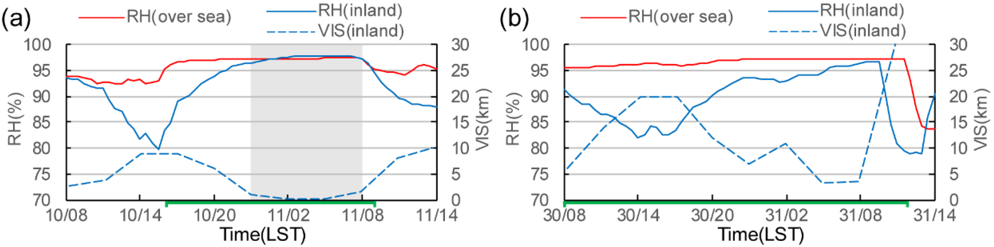
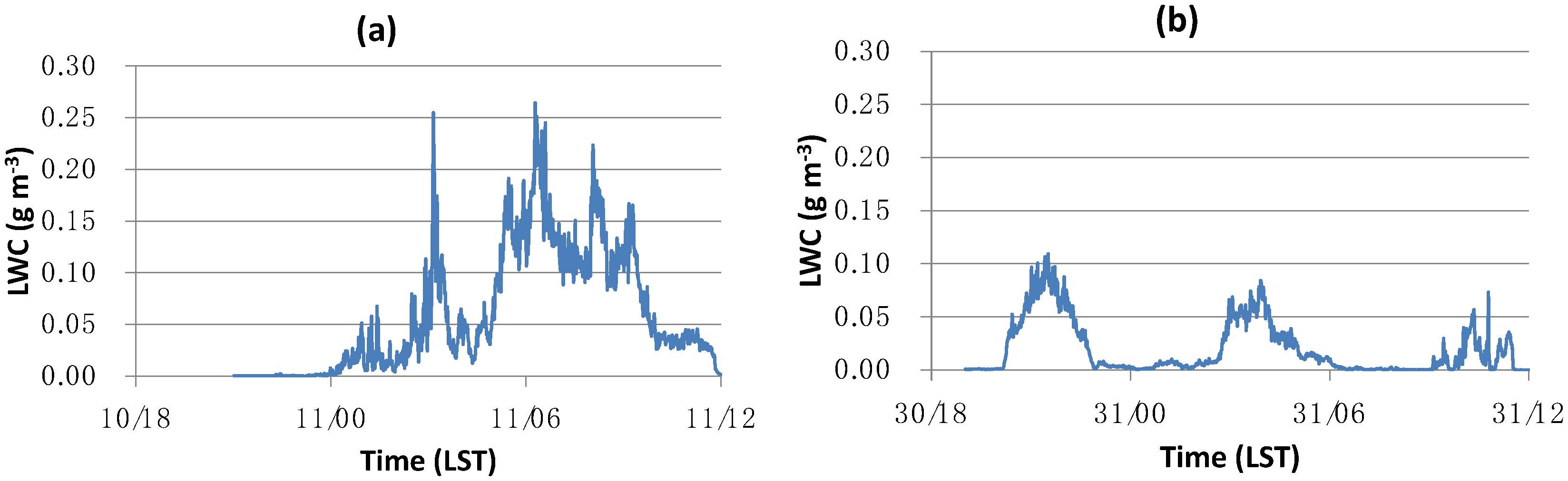
In both cases, the synoptic conditions involved warm, moist air from a warmer SST region advecting to a colder SST area at the coast, forming sea fog. But, the inland fog case had larger horizontal advection of water vapor over the land and about 80% low-cloud coverage.
(2)
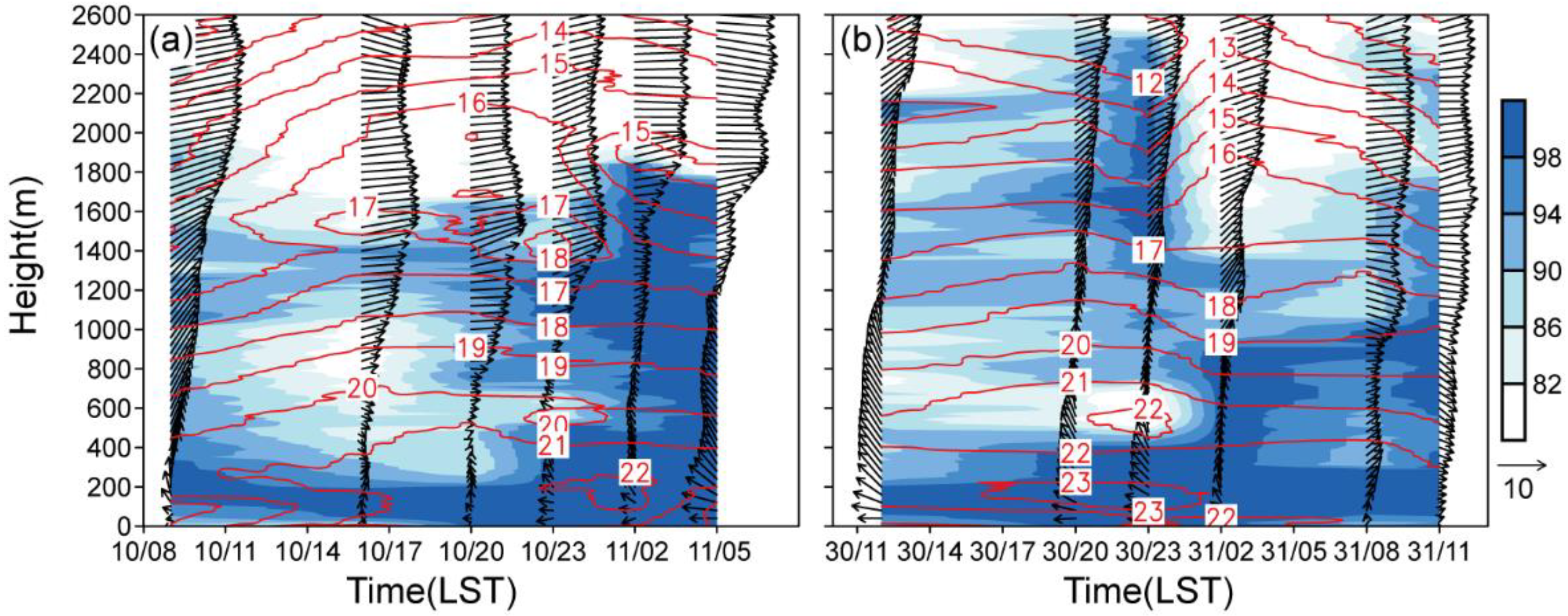
The surrounding boundary layer was important. Both sea-fog cases had low wind speeds and a small TKE. The small TKE allowed the vapor to accumulate close to the surface and maintain the local cooling effect, eventually producing fog.
(3)
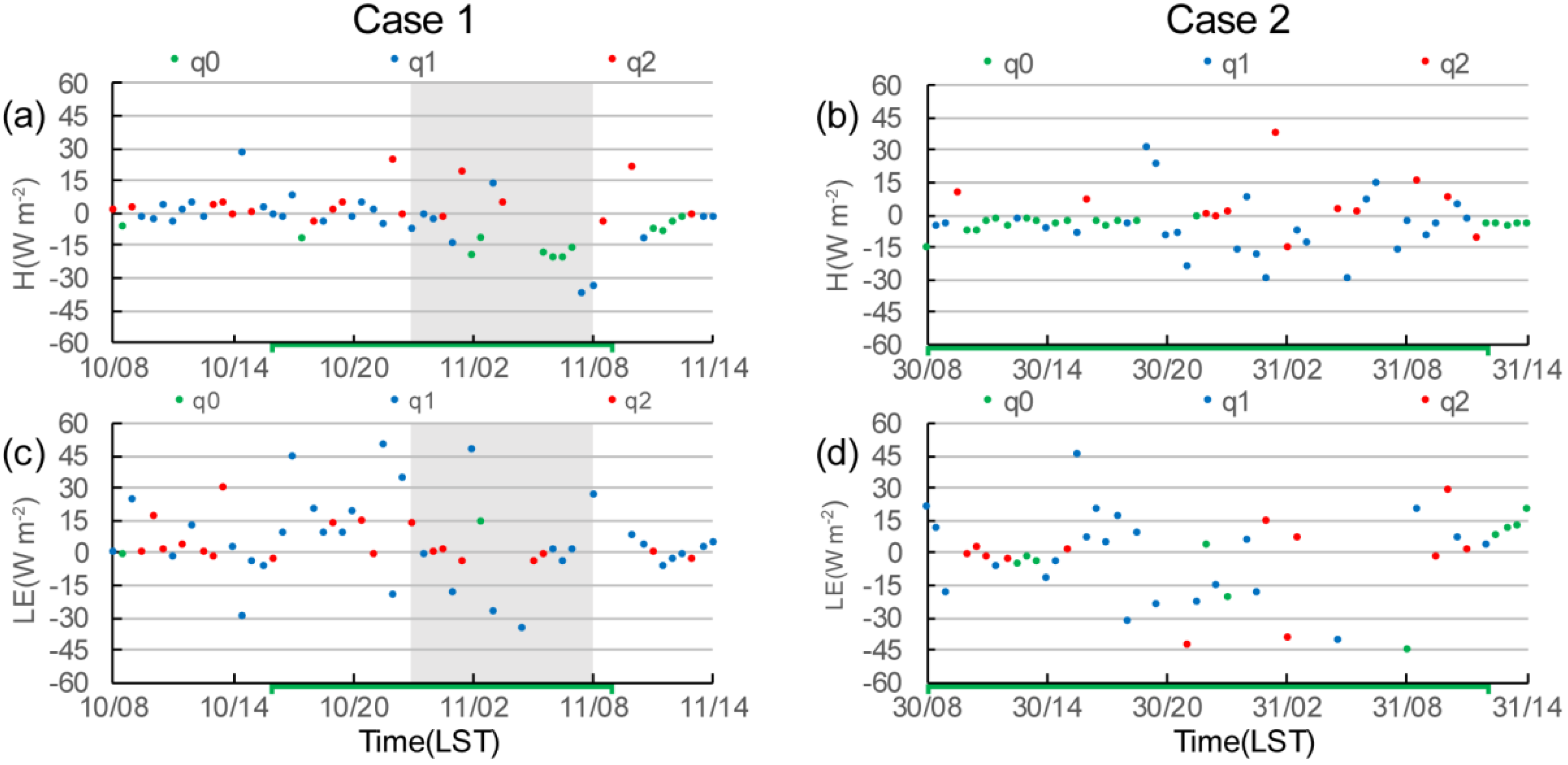
Both cases had radiative cooling of the ground, but the inland fog case had a downward energy flux at night, with the land surface cooling the atmosphere. The non-fog case had the opposite flux. The fog case also had lower soil temperature and higher soil humidity.
Although both sea fogs transported vapor inland over an extensive span of coast, inland fog formed only in some areas. This nonuniformity of the fog might due to nonuniformities in surface conditions such as local cooling and boundary-layer conditions.
This study analyzed how sea fog can influence inland-fog formation with the aim of determining the relationship between the two fogs. In addition to the large-scale influence from sea fog, local conditions are critical to inland-fog formation. This finding suggests that forecasters should pay more attention to the local meteorological conditions and the soil conditions under such a synoptic background. These results are based on just two cases, and thus should be evaluated against more cases, but the results may be helpful for coastal forecasters.

Author Contribution

Conceptualization, H.H., S.Z.; Methodology, H.H., S.Z.; Software, J.S.; Formal Analysis, J.S., H.H.; Data Curation, W.M.; Writing-Original Draft Preparation, J.S., H.H.; Writing-review & Editing, J.S., H.H.; Funding Acquisition, H.H.

Acknowledgments

Special thanks to the crew of the Marine Meteorological Science Experiment Base at Bohe for their help in conducting the field program and providing the data. This study was supported jointly by the National Natural Science Foundation of China (Grants 41675021, 41576108, and 41675019), subproject of the science and technology pilot project of the Chinese Academy of Sciences (Grant XDA11010403), the Meteorological Sciences Research Project (Grant GRMC2017M04), and the innovation team of forecasting technology for typhoon and marine meteorology of the Guangdong Provincial Meteorological Bureau.

Conflicts of Interest

The authors declare no conflict of interest.

References

  1. Lewis, J.M.; Koračin, D.; Redmond, K.T. Sea fog research in the United Kingdom and United States: A historical essay including outlook. Bull. Am. Meteorol. Soc. 2004, 85, 395–408. [Google Scholar] [CrossRef]
  2. Bergot, T. Quality assessment of the Cobel-Isba numerical forecast system of fog and low clouds. Pure Appl. Geophys. 2007, 164, 1265–1282. [Google Scholar] [CrossRef]
  3. Gultepe, I.; Tardif, R.; Michaelides, S.C.; Cermak, J.; Bott, A.; Bendix, J.; Müller, M.D.; Pagowski, A.; Hansen, B.; Ellrod, G.; et al. Fog research: A review of past achievements and future perspectives. Pure Appl. Geophys. 2007, 164, 1121–1159. [Google Scholar] [CrossRef]
  4. Koračin, D.; Dorman, C.E.; Lewis, J.M.; Hudson, J.G.; Wilcox, E.M.; Torregrosa, A. Marine fog: A review. Atmos. Res. 2014, 143, 142–175. [Google Scholar] [CrossRef]
  5. Lamb, H. Haars or North Sea Fogs on the Coasts of Great Britain; Meteorology Office Publication: Devon, UK, 1943. [Google Scholar]
  6. Leipper, D.F. Fog on the United States west coast: A review. Bull. Am. Meteorol. Soc. 1994, 75, 229–240. [Google Scholar] [CrossRef]
  7. Koračin, D.; Businger, J.A.; Dorman, C.E.; Lewis, J.M. Formation, evolution, and dissipation of coastal sea fog. Bound. Layer Meteorol. 2005, 117, 447–478. [Google Scholar] [CrossRef]
  8. Petterssen, S. Some Aspects of Formation and Dissipation of Fog; Geofysiske Publikasjoner: Olso, Norway, 1939. [Google Scholar]
  9. Jiusto, J.E. Fog Structure. In Clouds, Their Formation, Optical Properties, and Effects; Hobbs, P.V., Deepak, A., Eds.; Academic Press: New York, NY, USA, 1981; pp. 187–239. [Google Scholar]
  10. Duynkerke, P.G. Radiation fog: A comparison of model simulations with detailed observations. Mon. Weather Rev. 1991, 119, 324–341. [Google Scholar] [CrossRef]
  11. Bergot, T.; Guedalia, D. Numerical forecasting of radiation fog. Part I: Numerical model and sensitivity tests. Mon. Weather Rev. 1994, 122, 1218–1230. [Google Scholar] [CrossRef]
  12. Duynkerke, P.G. Turbulence, radiation and fog in Dutch stable boundary layers. Bound. Layer Meteorol. 1999, 90, 447–477. [Google Scholar] [CrossRef]
  13. Zhou, B.; Ferrier, B.S. Asymptotic analysis of equilibrium in radiation fog. J. Appl. Meteorol. Climatol. 2008, 47, 1704–1722. [Google Scholar] [CrossRef]
  14. Steeneveld, G.J.; Wokke, M.J.J.; Groot Zwaaftink, C.D.; Pijlman, S.; Heusinkveld, B.G.; Jacobs, A.F.G.; Holtslag, A.A.M. Observations of the radiation divergence in the surface layer and its implication for its parameterization in numerical weather prediction models. J. Geophys. Res. 2010, 115, D06107. [Google Scholar] [CrossRef]
  15. Sun, J.X.; Huang, H.J.; Zhang, S.P.; Liu, J.W.; Wang, Q. Impact of sea fog on coastal area: Analysis of two cases over the Yellow Sea in spring 2008. Oceanol. Limnol Sin. 2017, 48, 483–497. (In Chinese) [Google Scholar]
  16. Wang, B.H. Sea Fog; China Ocean Press: Beijing, China, 1985; p. 330. [Google Scholar]
  17. Writing Group of Guangdong Provincial Meteorological Bureau. Manual of Weather Forecast Technology in Guangdong Province; China Meteorological Press: Beijing, China, 2006; p. 526. [Google Scholar]
  18. Zhang, G.C. The progress of fog forecast operation in China. Adv. Meteorol. Sci. Technol. 2016, 6, 42–48. (In Chinese) [Google Scholar] [CrossRef]
  19. Huang, J.; Chan, P. Progress of marine meteorological observation experiment at Maoming of South China. J. Trop. Meteorol. 2011, 17, 418–429. [Google Scholar]
  20. Huang, J.; Wang, B.; Zhou, F.X.; Huang, F.; Lv, W.H.; Huang, H.M.; Huang, H.J.; Yang, Y.Q.; Mao, W.K. Turbulent heat exchange in a warm sea fog event on the coast of South China. Chin. J. Atmos. Sci. 2010, 34, 715–725. (In Chinese) [Google Scholar]
  21. Huang, H.J.; Liu, H.N.; Jiang, W.M.; Huang, J.; Mao, W.K. Characteristics of the boundary layer structure of sea fog on the coast of Southern China. Adv. Atmos. Sci. 2011, 28, 1377–1389. [Google Scholar] [CrossRef]
  22. Huang, H.J.; Liu, H.N.; Huang, J.; Mao, W.K.; Bi, X.Y. Atmospheric boundary layer structure and turbulence during sea fog on the Southern China coast. Mon. Weather Rev. 2015, 143, 1907–1923. [Google Scholar] [CrossRef]
  23. Huang, H.J.; Mao, W.K. The South China sea monsoon experiment—Boundary layer height (SCSMEX-BLH): Experimental design and preliminary results. Mon. Weather Rev. 2015, 143, 5035–5053. [Google Scholar] [CrossRef]
  24. Bolton, D. The computation of equivalent potential temperature. Mon. Weather Rev. 1980, 108, 1046–1053. [Google Scholar] [CrossRef]
  25. Foken, T.; Gӧckede, M.; Mauder, M.; Mahrt, L.; Amiro, B.; Munger, W. Post-field data quality control. In Handbook of Micrometeorology: A Guide for Surface Flux Measurement and Analysis; Lee, X.H., Massman, W., Law, B., Eds.; Kluwer Academic Publishers: Dordrecht, The Netherlands, 2004; pp. 181–208. [Google Scholar]
  26. Bessho, K.; Date, K.; Hayashi, M.; Ikeda, A.; Imai, T.; Inoue, H.; Kumagai, Y.; Miyakawa, T.; Murata, H.; Ohno, T.; et al. An introduction to Himawari-8/9—Japan’s new-generation geostationary meteorological satellites. J. Meteorol. Soc. Jpn. 2016, 94, 151–183. [Google Scholar] [CrossRef]
  27. Zhang, S.; Yi, L. A comprehensive dynamic threshold algorithm for daytime sea fog retrieval over the Chinese adjacent seas. Pure Appl. Geophys. 2013, 170, 1931–1944. [Google Scholar] [CrossRef]
  28. Wu, X.; Li, S. Automatic sea fog detection over Chinese adjacent oceans using Terra/MODIS data. Int. J. Remote Sens. 2014, 35, 7430–7457. [Google Scholar] [CrossRef]
  29. Gao, S.H.; Wu, W.; Zhu, L.L.; Fu, G.; Huang, B. Detection of nighttime sea fog/stratus over the Huang-hai Sea using MTSAT-1R IR data. Acta Oceanol. Sin. 2009, 28, 23–35. [Google Scholar]
  30. Thiébaux, J.; Rogers, E.; Wang, W.Q.; Katz, B. A new high-resolution blended real-time global sea surface temperature analysis. Bull. Am. Meteorol. Soc. 2003, 84, 645–656. [Google Scholar] [CrossRef]
  31. Draxler, R.R.; Hess, G.D. An overview of the HYSPLIT_4 modeling system of trajectories, dispersion, and deposition. Aust. Meteorol. Mag. 1998, 47, 295–308. [Google Scholar]
  32. Stull, R.B. An Introduction to Boundary Layer Meteorology; Kluwer Academic Publishers: Norwell, The Netherlands, 1988; p. 666. [Google Scholar]
  33. Ramage, C.S. Monsoon Meteorology; Academic Press: New York, NY, USA, 1971; p. 296. [Google Scholar]
  34. Arya, S.P. Introduction to Micrometeorology; Academic Press: San Diego, CA, USA, 2001; p. 415. [Google Scholar]
Figure 1. Observational site locations and close views. (a) Observational site A location (gray cross) on the southern China coast. (b) The coastal site A is the Marine Meteorological Science Experiment Base (MMSEB) (21.45° N, 111.32° E, 7.0 m MSL), the oversea site B is the Integrated Observation Platform for Marine Meteorology (IOPMM) (21.44° N, 111.39° E, operated by MMSEB), and the inland site C is the Dianbai National Climate Observatory (DNCO) (21.55° N, 110.99° E, 31.6 m MSL). Distances from different locations and from coastal lines (from Google Earth). (c) Close view of oversea site B (IOPMM); the upper-right corner of the image is the mounting position of the Gill Windmaster Pro and Li-cor 7500A instruments at the 23.4 m level (main photo courtesy of Weikang Mao on 27 June 2014). (d) Close view of inland site C (DNCO); the upper-right corner of the image is the mounting position of the Gill Windmaster Pro and Li-cor 7500A instruments at the 10 m level (main photo courtesy of Weikang Mao on 20 January 2017).
Atmosphere 09 00344 g001
Figure 2. Wind vectors (m s−1), water-vapor mixing ratio (shaded, g kg−1), and air pressure at sea-surface level (hPa). (a) 1400 LST March 10. (b) 1400 LST Mar 30. (c) 0200 LST Mar 11. (d) 0200 LST 31 March (with cold-front location). (e) 1400 LST March 11. (f) 1400 LST 31 March (From the FNL on 1° × 1° grid spacing datasets.). “A” is the coastal site.
Atmosphere 09 00344 g002
Figure 3. Visible cloud image from Himawari-8 and retrieval of the fog-cloud based on the Himawari-8 data of case 1 (left column) and case 2 (right column). (a) 1600 LST 10. (b) 1600 LST 30 March. (c) 0200 LST 11 March. (d) 0200 LST 31 March. (e) 0900 LST 11 March. (f) 0900 LST 31 March (A is the coastal site.).
Atmosphere 09 00344 g003
Figure 4. Fog and light-fog visibilities (km) at various inland and coastal stations during the two sea-fog periods. (a) Case 1. (b) Case 2. The “+” is inland site C (DNCO). Red denotes fog; black is light fog.
Atmosphere 09 00344 g004
Figure 5. Relative humidity over sea and inland, and visibility inland. (a) Case 1. (b) Case 2. RH is relative humidity, VIS is visibility. The green line indicates the sea-fog period defined as RH > 95% over sea, the grey shading indicates inland fog defined as RH > 96.5%.
Atmosphere 09 00344 g005
Figure 6. Airflow trajectories to inland site C with background of daily average sea-surface temperatures (°C). (a) Sea-surface temperature (SST) on March 10. Dotted lines denote 48 h backward trajectories of airflow at 20 m, 100 m, and 300 m heights from 0200 LST 11 March. (b) Same as (a), except SST on 30 March and trajectories from 0200 LST 31 March. SSTs are from real-time global data on 0.083° × 0.083° grid-spacing datasets.
Atmosphere 09 00344 g006
Figure 7. Time-average horizontal advection of temperature (10−4 K s−1) and wind vectors (m s−1). Left column (a,c) is case 1, from 2000 LST Mar 10 to 0800 LST March 11. Right column (b,d) is case 2, from 2000 LST Mar 30 to 0800 LST March 31. Top row (a,b) is at 1000 hPa. Bottom row (c,d) is 975 hPa. The red line is the zero line for the sign of advection. (A is the coastal site).
Atmosphere 09 00344 g007
Figure 8. Same as Figure 7, except for time-average horizontal vapor transport (shaded, 10−4 g kg−1 s−1) and wind vectors (m s−1).
Atmosphere 09 00344 g008
Figure 9. Soundings at the coastal site during the two sea-fog cases. The red line is air temperature, the shading is relative humidity, and the vector is horizontal wind. (a) Case 1. (b) Case 2. Scales for RH (%) and wind (m s−1) are at right.
Atmosphere 09 00344 g009
Figure 10. Boundary-layer structure at the time of the highest fog top of each fog case. (a) 0500 LST 11 March 2017 of case 1. (b) 0200 LST 31 March 2017 of case 2. Horizontal lines: 1 = height of the thermal-turbulence interface (determined as θ e z = 0 ); 2 = top of the fog (determined as RH = 98%, the same as 3 and 4), 3 = cloud base, 4 = cloud top. Symbols: T = temperature (K), θe = potential equivalent temperature (K), q = mixing ratio (kg kg−1), Wd = wind direction (°), Ws = wind speed (m s−1), RH = relative humidity (%), and height = AGL (m).
Atmosphere 09 00344 g010
Figure 11. Meteorological parameters and turbulence characteristics of case 1 (left column) and case 2 (right column) over sea and inland. (a,b) T10m = air temperature at 10 m AGL, T13.4m = air temperature at 13.4 m MSL. (c,d) WD, WS; (e,f) TKE; (g,h) rainfall = the rainfall in an hour. The green line indicates the sea-fog period, the grey shading indicates the inland-fog period.
Atmosphere 09 00344 g011
Figure 12. Sensible- and latent-heat fluxes over sea (23.4 m MSL). (a) Case 1, sensible. (b) Case 2, sensible. (c) Case 1, latent. (d) Case 2, latent. Dots are the flux values, averaged over 30 min. Missing data are either out of range or doubtful. Colors mark the quality flags of the fluxes, with q0 = green (see labels at top) the highest quality, q2 = red the lowest (see Table 2 for details). The green line indicates the sea-fog period, the grey shading indicates the inland-fog period.
Atmosphere 09 00344 g012
Figure 13. Observed liquid-water content (LWC) at coast site A (MMSEB) of the two sea-fog cases (Plotted are 1 min averages of 1 s data). (a) Case 1. (b) Case 2.
Atmosphere 09 00344 g013
Figure 14. Sensible- and latent-heat fluxes inland (10 m AGL). (a) Case 1, sensible. (b) Case 2, sensible. (c) Case 1, latent. (d) Case 2, latent. Averaging interval for the fluxes is 30 min. Missing data are either out of range or doubtful. Markings are the same as those in Figure 12.
Atmosphere 09 00344 g014
Figure 15. Land–atmosphere exchange characteristics at the inland site C. (a,b) Air (10 m AGL) and soil temperatures (5 and 10 cm depths) for cases 1 (left) and 2 (right). (c,d) Soil heat flux (HG, positive downward) and net radiation ( R N , positive downward) for both cases. (e,f) Soil volumetric water content (VWC) at 5 cm depth for both cases. The green line indicates the sea-fog period, the grey shading indicates the inland-fog period.
Atmosphere 09 00344 g015
Table 1. The observation sites, instruments, and data.
Instrument Type or Measurement VariablesMake and ModelObservation Sites and Nominal Height(s)
MMSEB (A)IOPMM (B)DNCO (C)
Ultrasonic Anemometer, Infrared CO2/H2O AnalyzersU.K. Gill Windmaster Pro; USA LI-COR LI-7500A——23.4 m MSL *10 m AGL **
GPS SondeFinland Vaisala RS-927 m MSL————
RadiometerNetherlands Kipp and Zonen CMP22/CGR4; CNR_41.5 m AGL12 m MSL1.5 m AGL
Gradients of Wind, Temperature, and HumidityUSA RM. Young 05106; Finland Vaisala HMP45d——13.4, 16.4, 20.0, 27.3 m MSL10 m AGL
PressureUSA Setra Setraceram CS100——13 m MSL1.5 m AGL
Rain gaugeUSA Campbell TB4——12 m MSL1.5 m AGL
Ground Temperature and HumidityUSA Campbell 109SS; Campbell CS616−5, −10, −20, −40 cm AGL——−5, −10, −20, −40 cm AGL
Skin TemperatureUSA Campbell IRR-P——8 m MSL1.5 m AGL
Soil Heat-Flux PlateUSA Campbell HFP01SC————−5 cm AGL
Auto Meteorological Station (six variables)China Guangdong Observation Center, WP31031.5 m AGL——1.5 m AGL
VisibilityUSA Belfort Model 60001.5 m AGL————
Liquid-Water ContentUSA DMT Model FM-1201.5 m AGL————
DataloggerUSA Campbell Scientific CR30007 m MSL13 m MSL 1.5 m AGL
* MSL: mean sea level. ** AGL: above-ground level.
Table 2. Overall quality flags of the EddyPro 6.2 software used in the turbulence analyses.
RNcov (%) *ITCσ (%) **QA/QC FlagData QualityThis Study
≤30≤300Highq0
≤100≤1001Moderateq1
>100>1002Lowq2
* RNcov is used to evaluate the steady state of turbulence. ** ITCσ is used to evaluate the integral turbulence characteristic. More information is available in Reference [25].
Table 3. Measurement goals and analysis periods (LST) at the three observation sites for both cases of sea fog.
Observation SiteGoalCase 1Case 2
CoastBoundary layer structure (GPS sonde release times)0900, 1600, 2000, 2300 LST 10 March; 0200, 0500 LST 11 March 1200, 2000, 2300 LST 30 March; 0200, 0800, 1100 LST 31 March
OverseaTurbulence near the sea surface0800 LST 10 March-1400 LST 11 March 0800 LST 30 March-1400 LST 31 March
InlandTurbulence near the land surface0800 LST 10 March-1400 LST 11 March 0800 LST 30 March-1400 LST 31 March
Table 4. Weather observations inland (site C) during the sea-fog events.
Before the Sea FogSea-Fog PeriodAfter Sea Fog
Case 1Day and time (LST)1400 LST March 101700 LST March 102000 LST March 102300 LST March 100200 LST March 110500 LST March 110800 LST March 111100 LST March 11
Cloud *300, 7/71000, 10/81000, 8/8-, 9/--, 9/--, 9/-1000, 8/81000, 8/8
Visibility (km)9.09.06.01.10.10.11.68.0
Weather phenomenaCloudyOvercastLight fogLight fogFogFogLight fogOvercast
Case 2Day and time (LST)1700 LST March 302000 LST March 302300 LST March 300200 LST March 310500 LST March 310800 LST March 311100 LST March 311400 LST March 31
Cloud300, 7/7300, 6/6-, 9/--, 9/--, 9/-1000, 8/8300, 7/7300, 7/7
Visibility (km)20.012.07.011.03.23.530.030.0
Weather phenomenaCloudyCloudyLight fogOvercastLight fogLight fogCloudyCloudy
* The upper number is cloud-base height (m), the lower fraction is total cloud cover/low-cloud amount (10/10; using a scale of 1 to 10; 10 means larger than 9.5, but less than 10; 0 means less than 0.5); “-” indicates no observation. All symbols follow the specifications for surface meteorological observations of China.

