Article

The Impacts of Smoke Emitted from Boreal Forest Wildfires on the High Latitude Radiative Energy Budget—A Case Study of the 2002 Yakutsk Wildfires

School of Earth and Atmospheric Sciences, Georgia Institute of Technology, Atlanta, GA 30332-0340, USA
*
Author to whom correspondence should be addressed.
Now at Department of Atmospheric Science, University of Wyoming, Laramie, WY 82071, USA.
Atmosphere 2018, 9(10), 410; https://doi.org/10.3390/atmos9100410
Submission received: 21 August 2018 / Revised: 13 October 2018 / Accepted: 15 October 2018 / Published: 19 October 2018
(This article belongs to the Special Issue Radiative Transfer in the Earth Atmosphere)

Abstract

:
We examine the 2002 Yakutsk wildfire event and simulate the impacts of smoke aerosols on local radiative energy budget, using the WRF-Chem-SMOKE model. When comparing satellite retrievals (the Surface Radiation Budget (SRB) dataset) with model simulations, we found that the agreement is generally good, except for the regions where the model predicts too few clouds or SRB misclassifies strong smoke plumes as clouds. We also found that the smoke-induced changes in upward shortwave fluxes at top of atmosphere (TOA) vary under different burning and meteorological conditions. In the first period of the fire season (9–12 August), smoke particles cause a warming effect around 3 W/m2, mainly through functioning as ice nuclei, which deplete the cloud water amount in the frontal system. At the beginning of the second period of the fire season (19–20 August), large amounts of pre-existing smoke particles cause a strong cooling effect of −8 W/m2. This is offset by the warming effect caused by relatively small amounts of cloud condensation nuclei increases, which promotes the rain formation and depletes the cloud water amount. After the cloud decks are well mixed with smoke plumes (21–22 August), the first indirect and direct effects of smoke together lead to a cooling of −10 W/m2. These results highlight the importance of meso-scale modeling efforts in estimating the smoke-induced changes in the radiative energy budget over high latitudes.

1. Introduction

Smoke aerosols emitted from wildfires in Siberia, Russia, can significantly affect the radiative energy budget over Europe and high latitude regions [1,2,3], directly via scattering and absorbing solar radiation (the direct effect) [4,5], and indirectly via altering cloud properties and the albedo (the indirect effect) [6,7]. The climate modeling results in [8] demonstrate that, over Siberia, the direct and indirect effects of smoke aerosols are as high as +1 W/m2 and −3 to −5 W/m2, respectively. However, it should be noted that, during the fire season in Siberia, smoke aerosols mainly interact with convective clouds associated with extratropical cyclones [9]. It is very challenging, if not impossible, for climate models to properly simulate the dynamics and thermodynamic characteristics of cyclones, because of the hydrostatic assumption and the relatively large grid spacing.
A few meso-scale modeling studies estimated the direct radiative effect of smoke aerosols over Russia, e.g., [10,11]. These studies focused on the most intense fire periods (a few days), and reported the daily averaged direct radiative effect of BB (biomass burning) aerosols as high as 70–150 W/m2. Although the results demonstrate the importance of smoke aerosols in altering the local radiative energy budget, these effects cannot be directly compared to the climatic effect of smoke aerosols estimated in [8]. To account for the large variability in daily fire activities over Siberia/Russia, at least one fire season, for instance, one month of the simulation is required for a thorough estimation of the direct radiative effect of smoke aerosols. Another shortcoming in these studies is that the impacts of smoke aerosols on cloud macro- and micro-physical properties are entirely or partially ignored. Without an accurate prediction of cloud fields in the domain, estimated direct radiative effect is biased (e.g., see discussions in [4]).
In our previous study [12] (hereinafter referred to as LS17), we simulated the 2002 Yakutsk wildfire case, using the WRF-Chem-SMOKE model [13] and examined the impacts of smoke on cloud properties. We found that, in different fire periods and under different meteorological conditions, the smoke-induced changes in cloud fields can be quite different, depending on the way that smoke plumes interact with cyclone-frontal systems. For instance, if a relatively large amount of the cloud condensation nuclei (CCN) but a relatively small amount of ice nuclei (IN) are activated from smoke particles, the cloud cells acquire longer lifetime and travel further downwind. Meanwhile, if both the large amount of CCN and IN are activated, the changes in the lifetime of cloud cells are small, but the locations of cloud cells will be significantly altered. This result indicates that a mesoscale modeling approach is required to properly and accurately estimate aerosol indirect effects and smoke-induced changes in the radiative energy budget over high latitudes.
In this study, we examine the WRF-Chem-SMOKE simulation of the 2002 Yakutsk wildfires event and focus on smoke-induced changes in the radiative energy budget. In Section 2, we discuss the modeling methodology, including how model is configured and how two simulation cases are designed, and describe satellite products used in this study. In Section 3, we first evaluate modeled upward shortwave fluxes at TOA (SWTOA↑) against satellite products, and then examine the smoke-induced changes in SWTOA↑ in two different fire periods. Finally, we conclude our main findings in Section 4.

2. Methodology

2.1. Model Configuration

The model setup and the configuration are exactly the same as in LS17. Here, we briefly describe how we configure and initialize the WRF-Chem-SMOKE model [13], which is built on the basis of the public WRF-Chem v3.3.1 model [14]. Our model domain is centered over Yakutsk, Russia (around 62° N, 130° E), covering a vast area of 4210 km (west-east) by 1810 km (north-south), with the 5 km horizontal resolution and 37 vertical layers. (The domain is shown in Figure 1 of LS17.) The model simulation is initialized with the FNL (final) reanalysis data (https://rda.ucar.edu/datasets/ds083.2/) and run from 1 August to 31 August 2002.
In the model, smoke aerosols are calculated by the MOSAIC 8-bin aerosol module [15], and treated as an internal mixture of black carbon (BC), organic matter (OM), and other inorganic matter (OIN). Smoke emissions are prepared based on the fire radiative power (FRP) technique [16]. By reconstructing the fire diurnal activity from active fires observed by MODIS onboard Terra and Aqua satellites, we prepare hourly smoke emission datasets as inputs for the WRF-Chem-SMOKE model. The radiative effect (smoke as a shortwave (SW) absorber) and microphysical effect (smoke as cloud condensation nuclei (CCN) and ice nuclei (IN)) of smoke particles are fully coupled with the Goddard SW radiation scheme [17,18] and the Morrison two-moment microphysical scheme [19]. Therefore, the direct and indirect effects of smoke aerosols are fully considered in this study.
In order to elucidate the effect of smoke aerosols on the radiative budget, we conduct two modeling cases: a reference case with all effects of smoke aerosols considered (SMOKE) and a smoke-free case (CLEAN) for comparison purposes.

2.2. Remote Sensing Data

In our study, we compare modeled radiative fluxes against the Global Energy and Water Exchange (GEWEX)-Surface Radiation Budget (SRB) version 3.0 dataset (https://gewex-srb.larc.nasa.gov/). The SRB datasets are derived based on two SW algorithms [20,21] and one LW algorithm [22] with cloud and radiance inputs from the International Satellite Cloud Climatology Project (ISCCP) and meteorological inputs from GMAO reanalysis dataset (http://gmao.gsfc.nasa.gov/). The SRB dataset provides radiative fluxes such as upward shortwave fluxes at TOA (SWTOA↑) and downward shortwave fluxes at the surface (SWSFC↓) every 3 hours at a spatial resolution of 1° × 1°.

3. Results: Assessment of the Impact of Smoke on Radiation

Burning and meteorological conditions during the 2002 Yakutsk wildfire season are thoroughly discussed in LS17. Mainly, there were two distinguishable fire periods: the fire period 1 (FP1, from 1 August to 11 August) and the fire period 2 (FP2, from 12 August to the end of August). During FP1, relatively small amounts of smoke particles were swirled into a relatively strong frontal system (FS1). In the beginning of FP2, the domain was under the influence of the strong blocking high-pressure system. Large amounts of smoke particles were released during this period interacted with a relatively weak frontal system (FS2), coming from the west of the domain later.

3.1. Comporison of Modeled Radiative Fluxs against the SRB Dataset
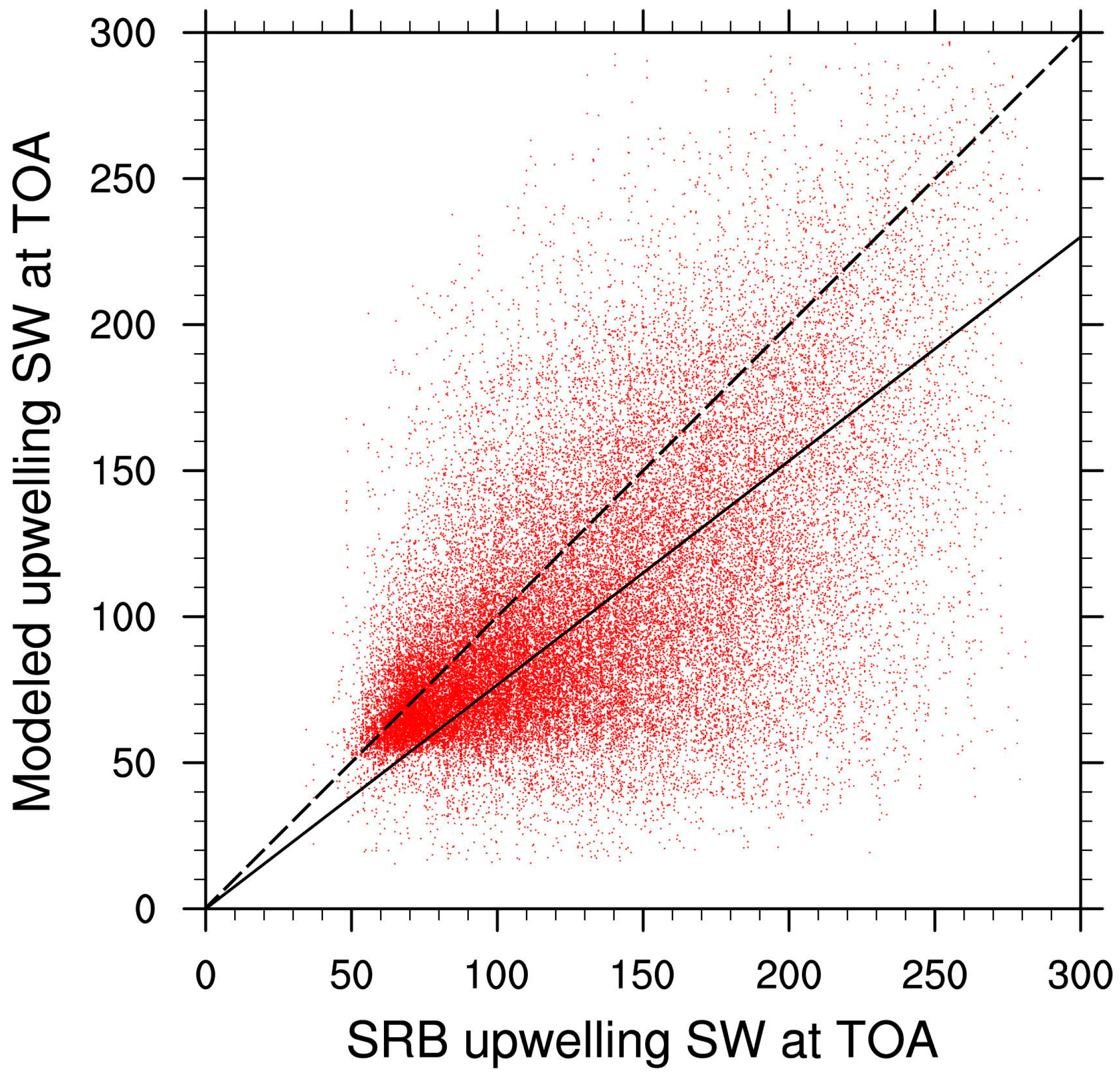
Firstly, in Figure 1 we compare the SRB SWTOA↑ and SWTOA↑ modeled by the SMOKE case for the entire simulation period (30 days). Please note that here we used positive values to represent SWTOA↑. Since we output modeled variables every two hours in contrast to the 3-h temporal resolution of the SRB dataset, for each day, we calculated the daily SWTOA↑ by averaging the SWTOA↑ at 0000, 0600, 1200, and 1800 UTC. In addition, to accommodate the spatial resolutions of the model grid and SRB dataset, we averaged all the model grids within each 1° × 1° grid. In total, 44,370 pairs of modeled daily SWTOA↑ and SRB daily SWTOA↑ are labeled in the scatter plot as shown in Figure 1. To compare modeled and SRB values, we conduct a regression analysis. The regression line, as shown by the black line in Figure 1, is set to pass (0,0) point. The regression coefficient between modeled and SRB daily SWTOA↑ equals 0.76, which indicates that the model tends to underestimate the magnitude of SWTOA↑. The fact that modeled SWTOA↑ is lower than SRB retrievals is very likely due to “too few, too bright” clouds modeled by numerical models [23], as in WRF-Chem-SMOKE. For example, our result is very similar to the study conducted in [24], which examines the radiative forcing of smoke in the Amazonia region using the WRF-Chem model. They found that modeled daily SWSFC↓ is 10% larger than SRB SWSFC↓, mainly due to optical thin clouds produced by the model. The smaller daily SWTOA↑ (e.g., the points below the regression line) in our study can be explained by the same reason.
Another possible explanation for the smaller magnitude of modeled daily SWTOA↑ compared to the SRB daily SWTOA↑ is due to the fact that SRB misclassifies the strong smoke plumes as cloud layers. Strictly speaking, the SRB dataset (v3.0) does not account for the real-time aerosol/smoke field, but only considers the standard aerosol profiles. 
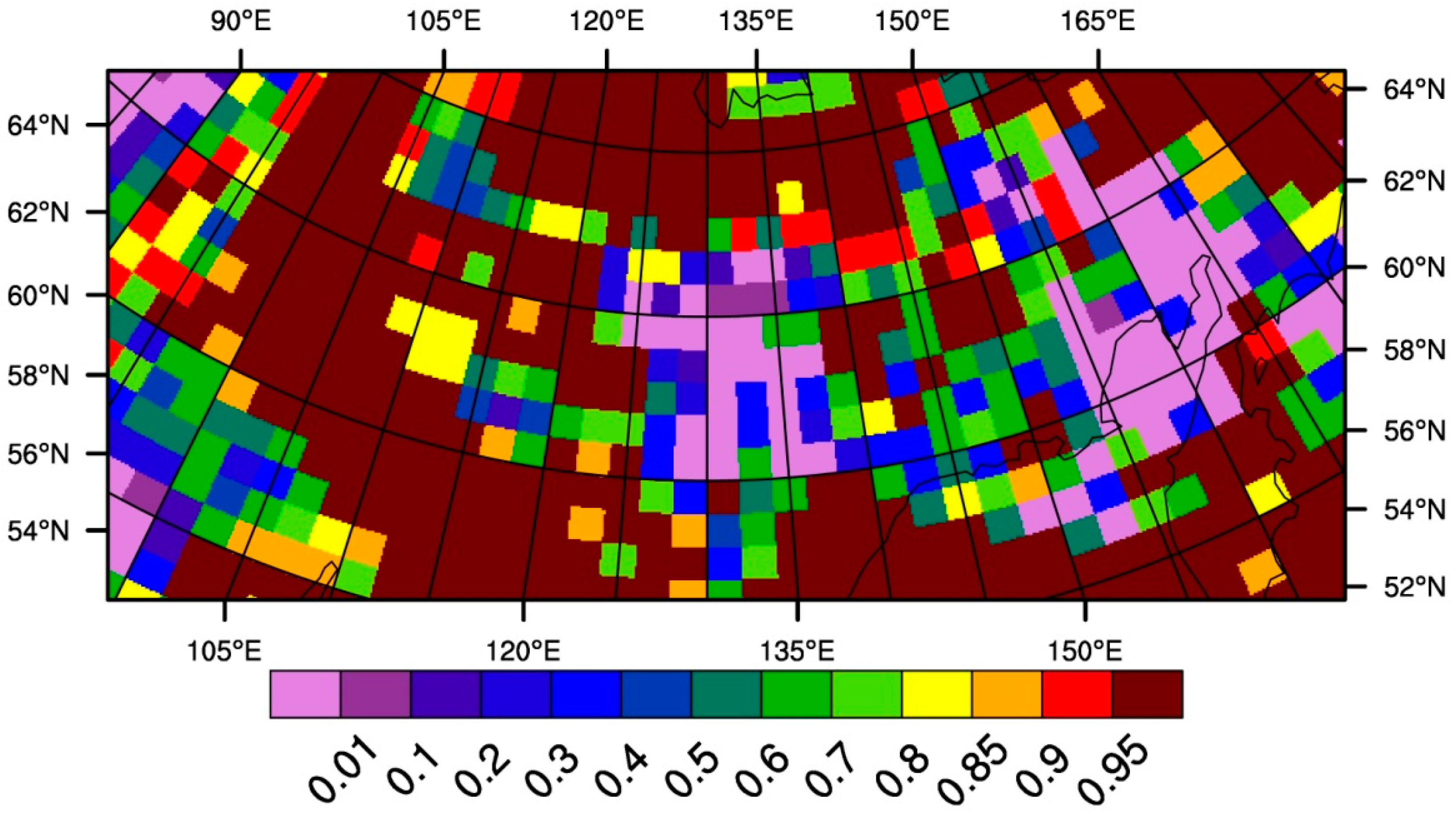
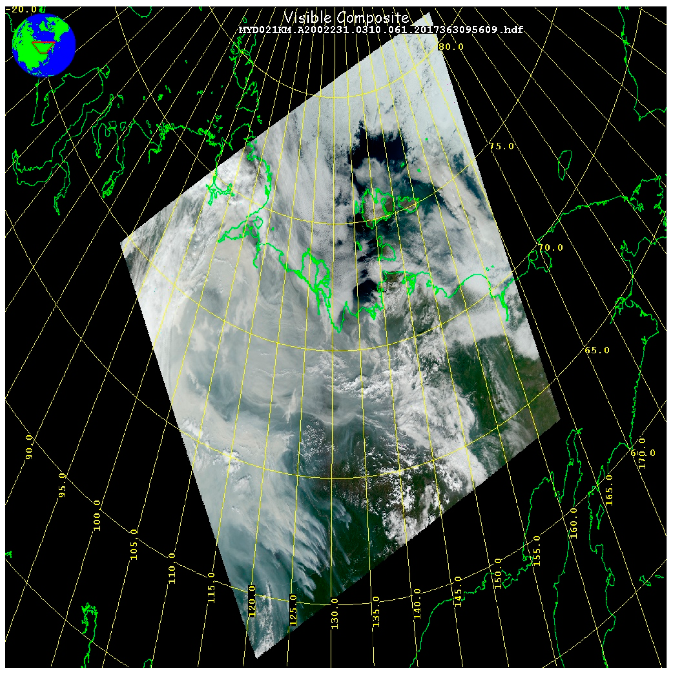
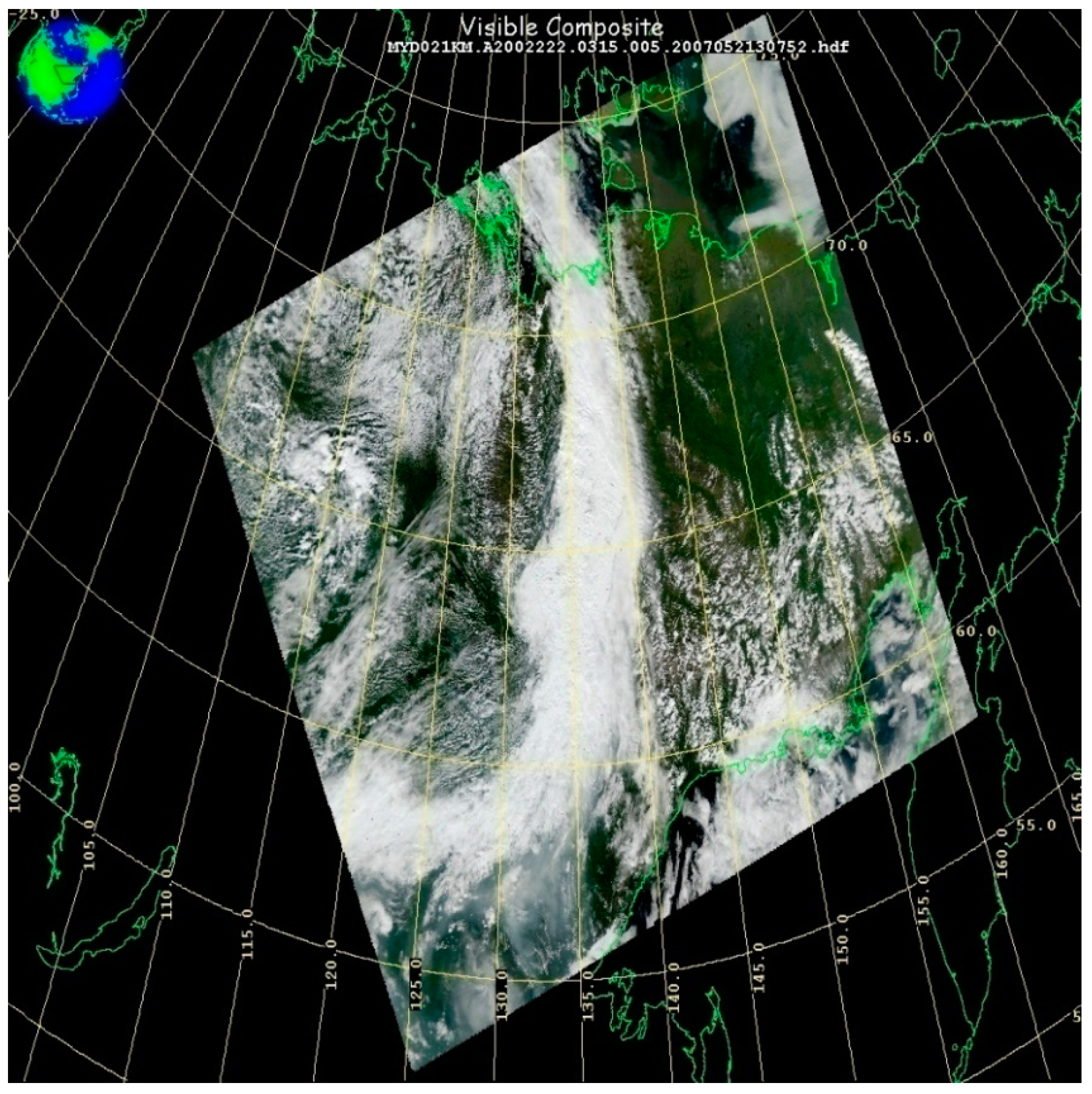
Figure 2 shows the SRB cloud fraction field at 0600 UTC on 19 August 2002. The SRB cloud fractions are retrieved from ISCCP and used as inputs in the SRB dataset. Compared to the true color image shown in Figure 3, we find that the SRB dataset classifies many 1° × 1° grids as having a cloud fraction higher than 0.95. However, the 1° × 1° grids in two regions (62° N–66° N, 115° E–125° E and 67° N–73° N, 110° E–150° E) are actually covered by strong smoke plumes. Because of the higher reflectivity associated with cloud pixels as compared to smoke pixels, the SRB dataset tends to overestimate SWTOA↑.
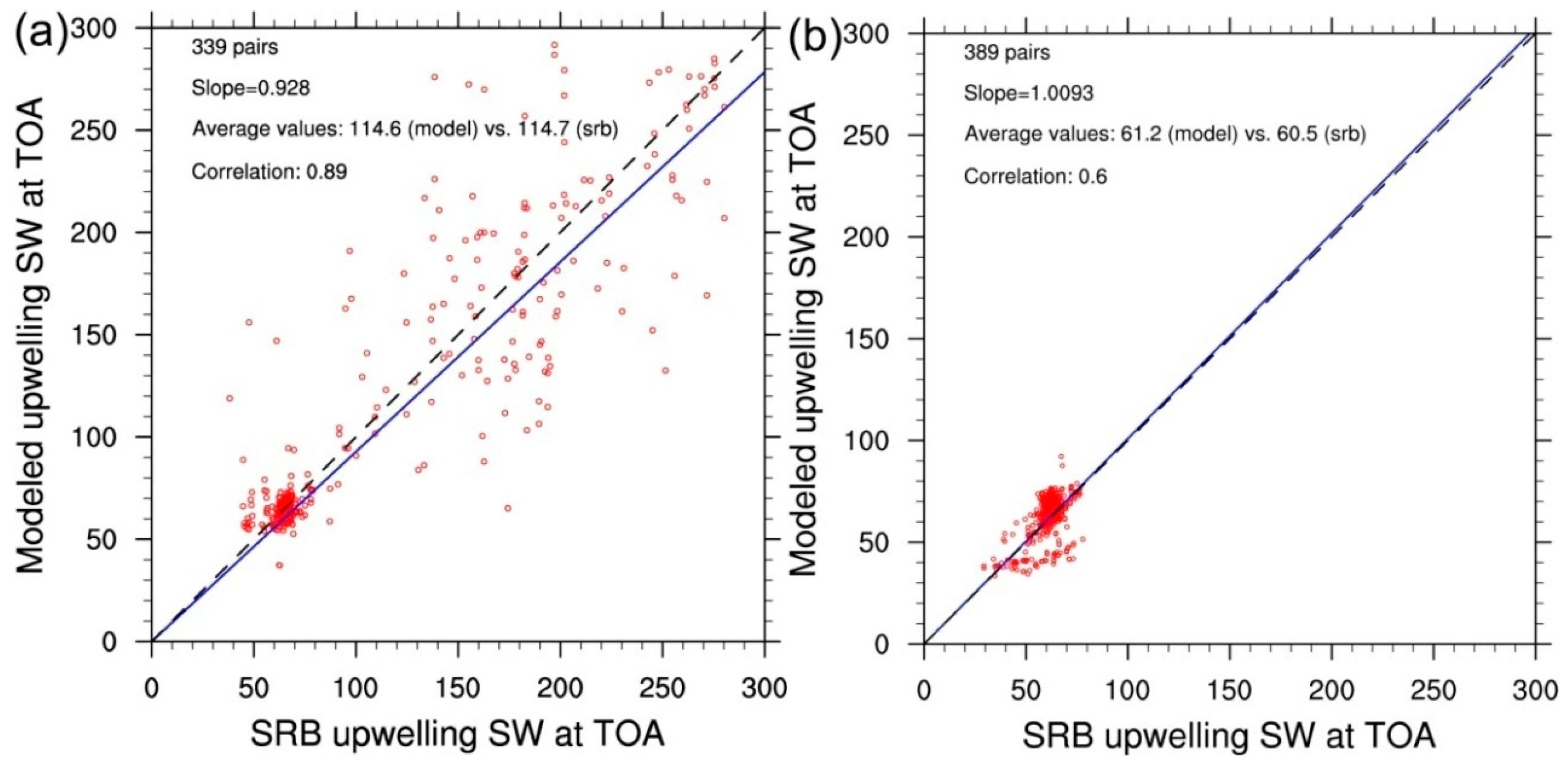
In order to prove our reasoning above, we further generated two more scatter plots, in which the SRB and modeled daily SWTOA↑ pairs were screened by different criteria. Firstly, we calculated the modeled cloud fractions, which are assumed as the ratios of the number of model grids with daily averaged total water path (TWP, only 0000, 0600, 1200, and 1800 UTC; four time steps) larger than 0.1 kg/m2 to the total number of model grids in each 1° × 1° grid. In Figure 4a, we label the SRB and modeled daily SWTOA↑ pairs, if the absolute differences between SRB retrieved cloud fraction and modeled cloud fractions are smaller than 0.05. The regression and correlation analyses, as well as average values, show that the modeled daily SWTOA↑ are reasonably modeled compared to SRB. In addition to all-sky radiative fluxes discussed above, the SRB dataset also provides clear-sky radiative fluxes, which are calculated by assuming the absence of clouds. Therefore, we select the modeled daily SWTOA↑ with daily averaged TWP and AOD in the 1° × 1° grid (only 0000, 0600, 1200, and 1800 UTC; four time steps), which are below 0.1 kg/m2 and 0.01, respectively, and compare the values against the clear-sky SRB daily SWTOA↑ in Figure 4b. Again, the statistical analyses show a good agreement between model simulation and the SRB dataset. These results highlight the importance of reasonable representations of modeled cloud properties.

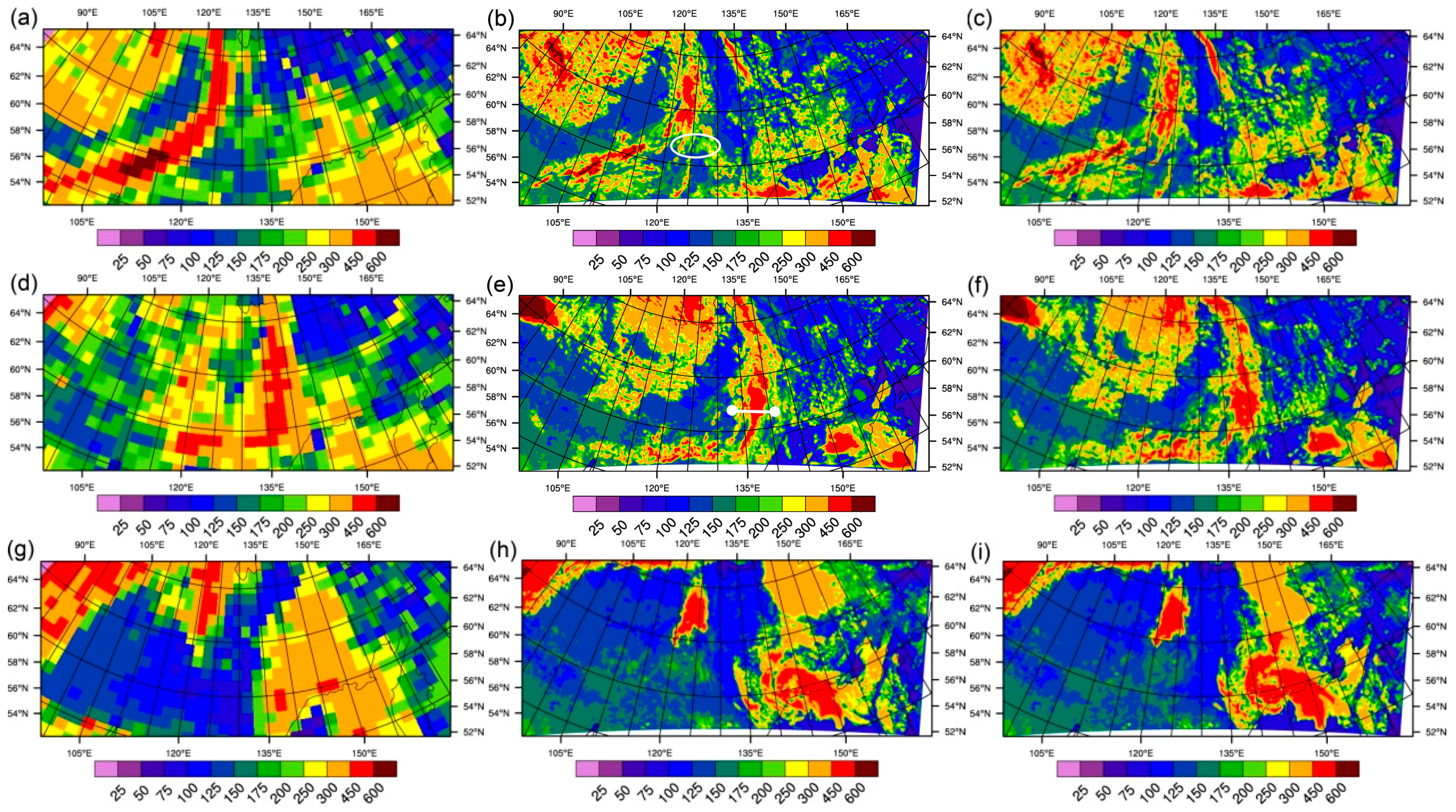
3.2. The Impact of Smoke on Radiative Fluxes during the Fire Period 1

Figure 5 shows SRB radiative fluxes in the first column and radiative fluxes modeled by SMOKE and CLEAN in the second and third columns at 0600 UTC on 9, 10 and 12 August. On 9 August, smoke plumes are located around 60° N–65° N, 125° E–135° E. In this region, the values of SWTOA↑ in the SRB dataset are around 150–200 W/m2 as shown in Figure 5a, while SWTOA↑ produced by the SMOKE and CLEAN cases, as shown in Figure 5b,c, are 175–250 W/m2 and 50–100 W/m2, the difference between which can be interpreted as the smoke direct radiative forcing in this region. When examining the SWTOA↑ associated with the frontal system (FS1 in LS17), we found that no significant difference exists between SMOKE and CLEAN, and both cases underestimate the magnitudes and the horizontal extents of SWTOA↑ compared to the SRB dataset.
By 0600 UTC 10 August, smoke particles have almost been swirled in FS1. As smoke particles being activated as CCN and IN (shown in Figure 4 in LS17), they strongly affect radiation fields via the indirect aerosol effect. The spatial distributions of SWTOA↑ modeled by SMOKE and CLEAN (shown in Figure 5e,f, respectively) significantly differ from each other in the lower portion of FS1. In particular, the lower portion of FS1 in CLEAN has the cloud coverage with the larger horizontal extent and appears further downwind. Comparing against the SRB dataset, we find that the SMOKE case performs much better in terms of simulating the spatial distributions of SWTOA↑. In order to explain how smoke, via functioning as CCN and IN, induces such differences in cloud properties and resulting SWTOA↑, we examine the smoke-induced changes in cloud properties along the cross-section labeled in Figure 5e (as shown by the white line from 131° E, 61° N to 137° E, 61° N).
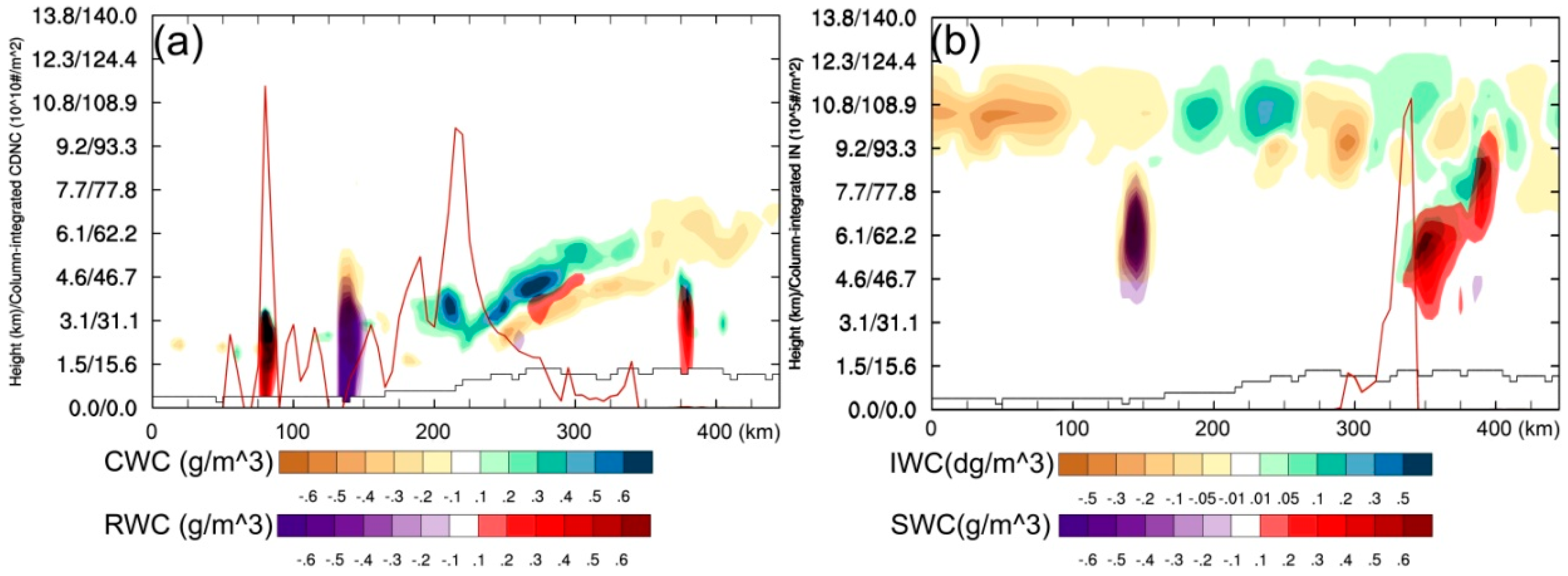
Similar to Figure 6 in LS17, Figure 6 in this study shows smoke-induced changes in cloud water content, rain water content, ice water content, and snow water content (CWC, RWC, IWC, and SWC) in color contours as well as column-integrated cloud droplet number concentration (CDNC) and IN in curve lines at 0600 UTC on 10 August 2002. As shown in Figure 6a,b, the CLEAN case produces a cloud cell with a large amount of RWC and SWC at 135 km along the X-axis, while the corresponding cloud cell in SMOKE, located around 145 km along the X-axis, contains a moderate amount of RWC, but it lacks the strong vertical development and SWC. This is probably due to the high CDNC, which suppress the collision-coalescence and riming processes in this region. As shown in Figure 6b, we find that a relatively large amount of IN is activated at the forward edge of the lower portion of FS1. As a result, the higher IN concentration promotes the formation of SWC and quickly depletes the water content in this region. In contrast, CLEAN produces a layer with a moderate amount of CWC. Therefore, the combined effects of CDNC and IN lead to the smoke-induced changes in cloud properties, which further cause differences in SWTOA↑ as shown in Figure 5e,f.
On 10 August 2002, according to the SRB dataset, values of SWTOA↑ behind (to the west of) FS1 are around 250–450 W/m2. These fairly high values are due to the presence of stratocumulus clouds behind the frontal system as shown in the MODIS true color image in Figure 7. However, both SMOKE and CLEAN fail to produce a considerable amount of the cloud coverage, which eventually causes underestimated SWTOA↑ behind FS1 on 10 August.
As discussed in LS17, by the time of 0400~0600 UTC 12 August 2002, the upper portion of FS1 has developed into a sub-polar vortex, while the lower portion of FS1 has become a mid-latitude cyclone system. As shown in Figure 5g, the magnitudes of SWTOA↑ associated with the mid-latitude cyclone are around 300~450 W/m2. (Values of SWTOA↑ in only a few 1° × 1° grids are higher than 450 W/m2.) When examining the SWTOA↑ modeled by SMOKE and CLEAN in the same region, we find that the magnitudes in both cases are higher than 450 W/m2, but lower than 600 W/m2 as shown in Figure 5h,i. However, it should be noted that the performance by SMOKE exceeds that by CLEAN on 12 August, since SMOKE produces fewer model grids with SWTOA↑ higher than 450 W/m2. This is probably due to the fact that IN activated from smoke particles keep depleting the cloud water within the cyclone.

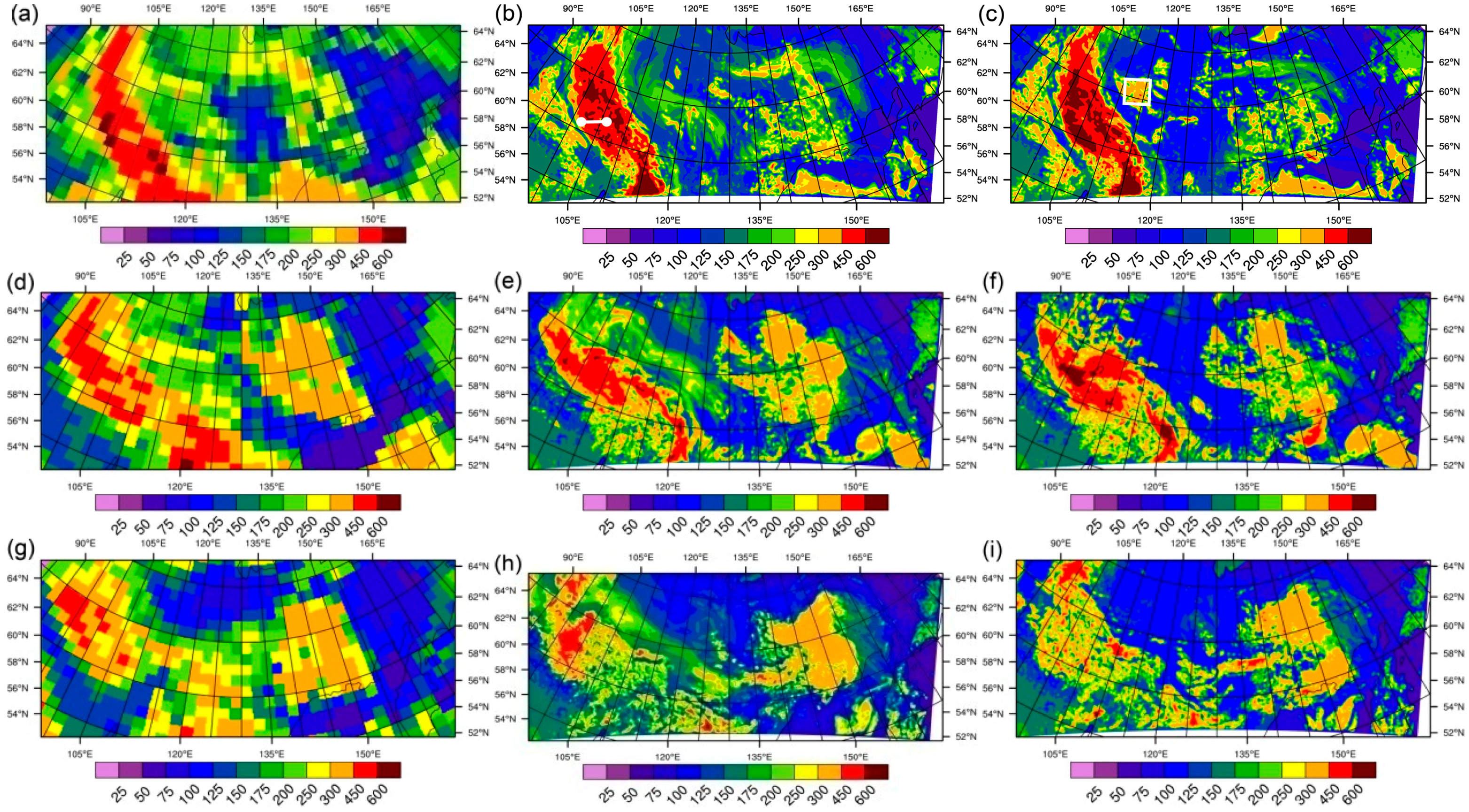
3.3. The Impact of Smoke on Radiative Fluxes during the Fire Period 2

On 19 August, dense smoke plumes cover a vast region and exert the significant radiative forcing at TOA and the surface. Meanwhile, around the western and eastern edges of the blocking high-pressure system, where the pressure cap is relatively weak, two cloud decks (shallow convections) appear, which are contaminated by smoke particles. The smoke-induced changes in radiative fluxes via the direct and indirect aerosol effects on 19 August and the following two days will be the focus of this section.
At 0600 UTC on 19 August, the SRB SWTOA↑ associated with the smoke plumes are around 175~250 W/m2, as shown in Figure 8a. It should be noted that the SRB SWTOA↑ are calculated by assuming the smoke plumes as clouds. Comparing against the SRB dataset, we find that the SMOKE case successfully reproduces the magnitudes and the spatial distribution of the SWTOA↑ field below 67° N, between 110° E~130° E, as shown in Figure 8b; however, SMOKE significantly underestimates the magnitudes of SWTOA↑ above 67° N, between 110° E and 125° E by about 100 W/m2. The difference between SRB and modeled SWTOA↑ is probably due to the false assumption of cloud layers in the SRB dataset or underestimations in modeled smoke AODs in this region. Apparently, the CLEAN case does not reproduce the SWTOA↑ associated with the smoke plume.
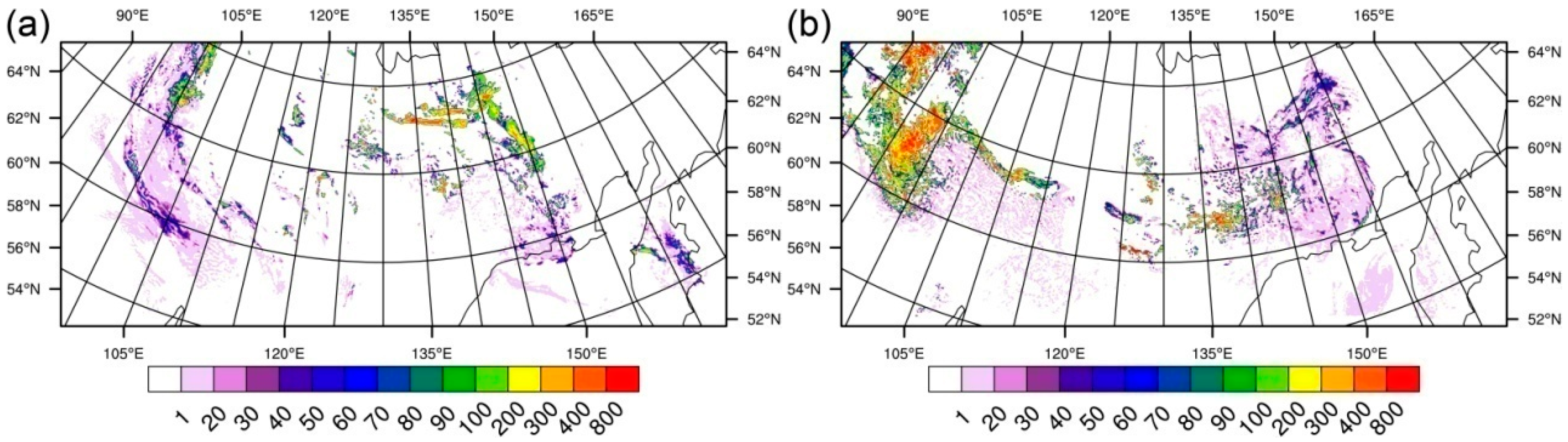
As shown in Figure 8b, around the eastern edge of the blocking high-pressure system, the liquid-phase cloud deck, which stretches from west (130° E) to east (150° E) along 68° N, is greatly affected by smoke particles. As shown in Figure 9a, large amounts of CDNC are activated from smoke particles within this cloud deck at 0600 UTC on 19 August. Due to the first indirect aerosol effect, the cloud deck in the SMOKE case becomes more reflective than the one in the CLEAN case. As a result, the values of SWTOA↑ produced by SMOKE are around 250 W/m2, which are much closer to the SRB SWTOA↑ as compared to CLEAN in this region.
When examining the cloud deck around the western edge of the blocking high-pressure system (from 67° N 100° E to 56° N 115° E), we find that this cloud deck, which is also in the liquid phase, is contaminated by a relatively small amount of smoke particles. Consequently, column-integrated CDNC activated from smoke particles are relatively low in this area (~4 × 10¹⁰ m−2). The values of SRB SWTOA↑ associated with this cloud deck are generally within 450–600 W/m2 as shown in Figure 8a. Therefore, we find that the SMOKE case performs better than the CLEAN case in simulating SWTOA↑, since the latter predicts too many model grids with SWTOA↑ higher than 600 W/m2 as shown in 
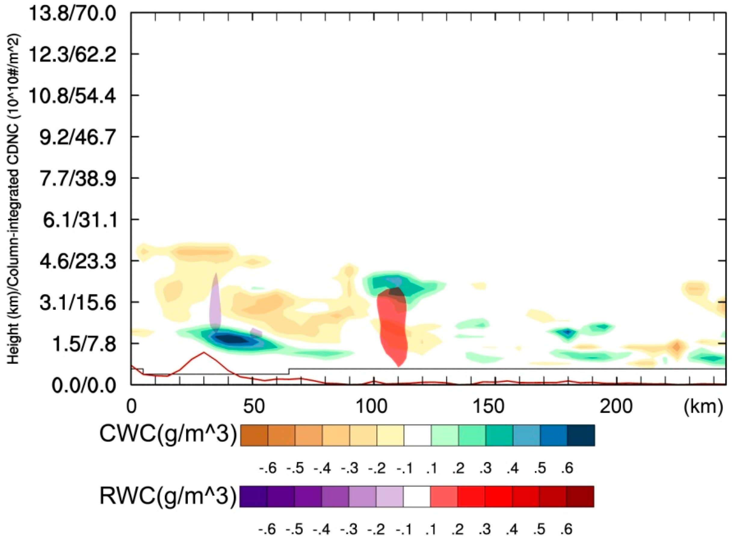
Figure 8c. In order to interpret smoke-induced changes in SWTOA↑, we examine smoke-induced changes in cloud properties (CWC, RWC, and column-integrated CDNC) along the cross-sections labeled in Figure 8b at 0600 UTC on 19 August. As shown in Figure 10, relatively low CDNC in the SMOKE case actually promote the rain formation, while more CWC is predicted by the CLEAN case in the cloud deck. Therefore, the cloud deck in the SMOKE case is optically thinner and less reflective than the one in CLEAN.
During the following two days (20 and 21 August), the direct aerosol effect of smoke remains significant. For example, magnitudes of SRB SWTOA↑ associated with the smoke plumes are still around 175–250 W/m2. The SMOKE case performs reasonably in predicting the magnitudes and the spatial distributions of radiative fluxes associated with the smoke plumes. The intensity of the cloud deck around the western edge of the blocking high-pressure system weakens on 20 and 21 August. For example, we find that the number of 1° × 1° grids with SRB SWTOA↑ higher than 450 W/m2 declines on 20 August compared to the previous day, and the shallow convective clouds degrade to stratocumulus clouds on 21 August. Comparing the SWTOA↑ modeled by SMOKE and CLEAN against the SRB dataset on 20 and 21 August, we find that the SMOKE case performs much better than the CLEAN case in simulating the SWTOA↑ associated with the cloud deck around the western edge of the blocking high-pressure system. Specifically, similar to the previous day on 19 August, the CLEAN case overestimates the number of model grids with SWTOA↑ higher than 600 W/m2 on 20 August as shown in Figure 8f. On 21 August, however, the CLEAN case underestimates the magnitudes of SWTOA↑ associated with the cloud deck between 90° E and 100° E below 65° N by 100–200 W/m2 as shown in Figure 8i. This is due to the fact that the stratocumulus clouds have been well mixed with the smoke plume by 21 August. High CDNC are activated from the smoke particles as shown in Figure 9b. Due to the first indirect aerosol effect, the albedo of the cloud deck in the SMOKE was higher.
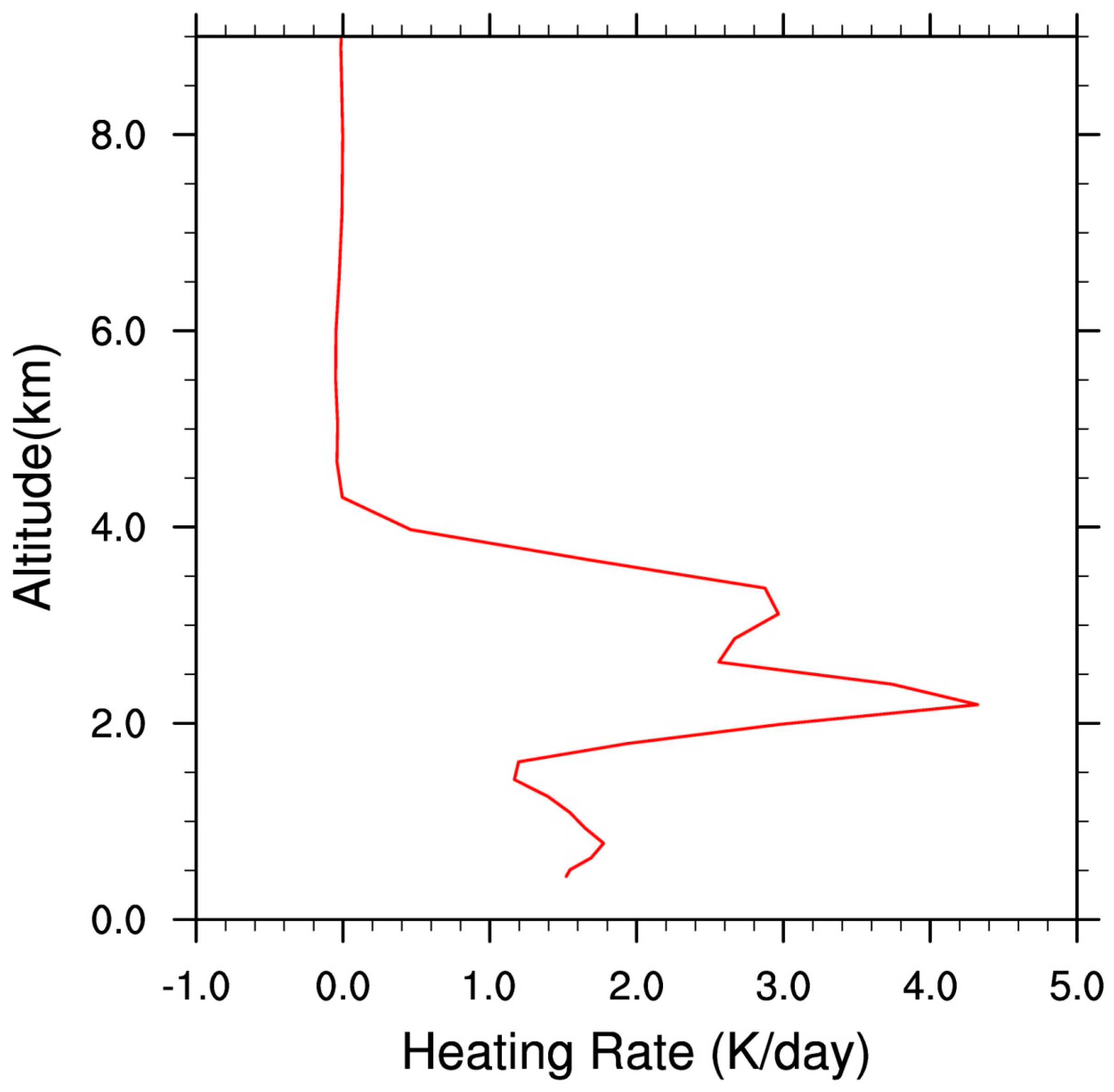
Although the microphysical effect of smoke is the focus of our study, we cannot rule out the importance of the semi-direct or the radiative effect of smoke. Here, we show one example of how the semi-direct effect of smoke completely suppresses the development of one short-lived shallow cloud deck. As shown in Figure 8c, the white square highlights one liquid-phase shallow cloud deck, which is only predicted by the CLEAN case at 0600 UTC on 19 August. The cloud deck has a cloud lifetime of less than 2 h, since it does not appear in the CLEAN case at 0400 UTC. In the same area, the SMOKE case predicts heavy smoke plumes for a few days. Therefore, in order to interpret the semi-direct effect of smoke on this cloud deck, we examine the difference in area-averaged heating profiles at 0400 UTC between SMOKE and CLEAN in Figure 11. Apparently, the strong smoke plumes in this area significantly heat the atmosphere. The difference in area-averaged heating profiles between the two cases peaked around 2 km above the terrain. As a result, very likely due to the stability of the atmosphere being increased by the presence of smoke, the development of the cloud deck was completely suppressed in the SMOKE case.

4. Discussion and Conclusions

In this study, we simulated the radiative forcing induced by large amounts of smoke particles released from the 2002 Yakutsk wildfire event, using the WRF-Chem-SMOKE model. By comparing against satellite retrievals, we found that model performs reasonably well in reproducing the radiation fields during the fire season considered.
We also examined the smoke-induced changes in radiative fluxes during the different periods of one fire season. We found that the relative importance of the direct and indirect aerosol effects of smoke varies under different fire regimes and meteorological conditions. Moreover, the indirect aerosol effect can either offset or add to the direct aerosol effect, depending on the CDNC/IN regimes. Therefore, it is critical to determine the total effect of smoke on the radiation fields. In order to summarize our findings, we calculated the smoke-induced changes in domain-averaged SWTOA↑ at 0600 UTC for four consecutive days for both FP1 and FP2, and defined these values as the total aerosol radiative effect (TARE). (It should be noted that we added a minus sign to the values so that the negative values correspond to the cooling effect.) In addition, we calculated the smoke-induced changes in domain-averaged SWTOA↑, but only for the model grids with a very small amount of cloudiness (TWP < 0.01 kg/m2, in both CLEAN and SMOKE), and defined the value as the direct aerosol radiative effect (DARE). The time series of TARE (red lines) and DARE (blue lines) for FP1 and FP2 are shown in Figure 12a,b, respectively. During FP1 (from 9 to 12 August), the direct effect of smoke causes a slight cooling effect at TOA. By 11 August, nearly all smoke particles emitted during FR1 have been swirled into the frontal system completely; therefore, the DARE value is close to zero on this day. When examining TARE, we found that the value remains positive across four days. This indicates that the indirect aerosol effect competes with and exceeds the direct aerosol effect of smoke. This is mainly because smoke particles acting as IN keep depleting the cloud water at the forward edge of the lower portion of the frontal system (FS1). For FP2, we only considered the western portion of the domain (<130° E), since it is affected by smoke for a shorter period than the eastern portion of the domain. DARE from 19 to 22 August causes a significant cooling effect at TOA, apparently due to the preexisting smoke plumes in the domain. During 19–20 August, the values of TARE are close to zero, indicating that the indirect aerosol effect compensates for the direct aerosol effect of smoke. This is actually due to the small amount of CDNC, which promotes the rain formation in shallow convections and cause cloud layers to be optically thinner. During 21–22 August, the values of TARE becomes negative. This is because large amounts of CDNC decrease the size of cloud droplets and increase the albedo of the cloud layers of stratocumulus, which are well mixed with smoke particles.
By comparing the model simulations against the SRB dataset, our study also demonstrates that the inclusion of the radiative and microphysical properties of smoke in meso-scale modeling can improve the simulation of radiation fields. More specifically, realistically modeled radiation fields require accurate predictions of the amount of smoke in the terrestrial state, the amount of smoke swirled in cloud layers, and the CCN/IN activations of smoke. Apparently, only a meso-scale model such as WRF-Chem-SMOKE is capable to achieve this goal.

Author Contributions

Conceptualization, Z.L. and I.N.S.; Methodology, Z.L. and I.N.S.; Writing—Original Draft Preparation, Z.L.; Writing—Review & Editing, Z.L. and I.N.S.; Visualization, Z.L.

Funding

Irina N. Sokolik acknowledges the support from NASA and NSF.

Conflicts of Interest

The authors declare no conflict of interest.

References

  1. Forkel, R.; Balzarini, A.; Baro, R.; Bianconi, R.; Curci, G.; Jimenez-Guerrero, P.; Hirtl, M.; Honzak, L.; Lorenz, C.; Im, U.; et al. Analysis of the WRF-Chem contributions to AQMEII phase 2 with respect to aerosol radiative feedbacks on meteorology and pollutant distributions. Atmos. Environ. 2015, 115, 630–645. [Google Scholar] [CrossRef]
  2. Kong, X.; Forkel, R.; Sokhi, R.S.; Suppan, P.; Baklanov, A.; Gauss, M.; Brunner, D.; Baro, R.; Balzarini, A.; Chemel, C.; et al. Analysis of meteorology-chemistry interactions during air pollution episodes using online coupled models within AQMEII phase-2. Atmos. Environ. 2015, 115, 527–540. [Google Scholar] [CrossRef] [Green Version]
  3. Palacios-Pena, L.; Baro, R.; Baklanov, A.; Balzarini, A.; Brunner, D.; Forkel, R.; Hirtl, M.; Honzak, L.; Lopez-Romero, J.M.; Montavez, J.P.; et al. An assessment of aerosol optical properties from remote-sensing observations and regional chemistry climate coupled models over Europe. Atmos. Chem. Phys. 2018, 18, 5021–5043. [Google Scholar] [CrossRef]
  4. Stone, R.S.; Anderson, G.P.; Shettle, E.P.; Andrews, E.; Loukachine, K.; Dutton, E.; Schaaf, C.; Roman, M.O., III. Radiative impact of boreal smoke in the Arctic: Observed and modeled. J. Geophys. Res. 2008, 113, D14S16. [Google Scholar] [CrossRef]
  5. Carslaw, K.S.; Boucher, O.; Spracklen, D.V.; Mann, G.W.; Rae, J.G.L.; Woodward, S.; Kulmala, M. A review of natural aerosol interactions and feedbacks within the Earth system. Atmos. Chem. Phys. 2010, 10, 1701–1737. [Google Scholar] [CrossRef] [Green Version]
  6. Penner, J.E.; Dickinson, R.E.; O’Neill, C.A. Effects of aerosol from biomass burning on the global radiation budget. Science 1992, 256, 1432–1434. [Google Scholar] [CrossRef] [PubMed]
  7. Andreae, M.O.; Rosenfeld, D. Aerosol–cloud–precipitation interactions, part 1. The nature and sources of cloud-active aerosols. Earth-Sci. Rev. 2008, 89, 13–41. [Google Scholar] [CrossRef]
  8. Jiang, Y.; Lu, Z.; Liu, X.; Qian, Y.; Zhang, K.; Wang, Y.; Yang, X.-Q. Impacts of global open-fire aerosols on direct radiative, cloud and surface-albedo effects simulated with CAM5. Atmos. Chem. Phys. 2016, 16, 14805–14824. [Google Scholar] [CrossRef]
  9. Gorbatenko, V.P.; Ippolitov, I.I.; Podnebesnykh, N.V. Atmospheric Circulation over Western Siberia in 1976–2004. Russ. Meteorol. Hydrol. 2007, 32, 301–306. [Google Scholar] [CrossRef]
  10. Péré, J.C.; Bessagnet, B.; Mallet, M.; Waquet, F.; Chiapello, I.; Minvielle, F.; Pont, V.; Menut, L. Direct radiative effect of the Russian wildfires and its impact on air temperature and atmospheric dynamics during August 2010. Atmos. Chem. Phys. 2014, 14, 1999–2013. [Google Scholar] [CrossRef] [Green Version]
  11. Toll, V.; Reis, K.; Ots, R.; Kaasik, M.; Männik, A.; Prank, M.; Sofiev, M. SILAM and MACC reanalysis aerosol data used for simulating the aerosol direct radiative effect with the NWP model HARMONIE for summer 2010 wildfire case in Russia. Atmos. Environ. 2015, 121, 75–85. [Google Scholar] [CrossRef]
  12. Lu, Z.; Sokolik, I.N. Examining the impact of smoke on frontal clouds and precipitation during the 2002 Yakutsk wildfires using the WRF-Chem-SMOKE model and satellite data. J. Geophys. Res. Atmos. 2017, 122, 12765–12785. [Google Scholar] [CrossRef]
  13. Lu, Z.; Sokolik, I.N. The effect of smoke emission amount on changes in cloud properties and precipitation: A case study of Canadian boreal wildfires of 2007. J. Geophys. Res. Atmos. 2013, 118, 11777–11793. [Google Scholar] [CrossRef]
  14. Grell, G.A.; Peckham, S.E.; Schmitz, R.; McKeen, S.A.; Frost, G.; Skamarock, W.C.; Eder, B. Fully coupled “online” chemistry within the WRF model. Atmos. Environ. 2005, 39, 6957–6975. [Google Scholar] [CrossRef]
  15. Zaveri, R.A.; Easter, R.C.; Fast, J.D.; Peters, L.K. Model for Simulating Aerosol Interactions and Chemistry (MOSAIC). J. Geophys. Res. 2008, 113, D13204. [Google Scholar] [CrossRef]
  16. Ichoku, C.; Kaufman, Y.J. A method to derive smoke emission rates from MODIS fire radiative energy measurements. IEEE Trans. Geosci. Remote Sens. 2005, 43, 2636–2649. [Google Scholar] [CrossRef]
  17. Chou, M.D.; Suarez, M.J.; Ho, C.H.; Yan, M.M.H.; Lee, K.T. Parameterizations for cloud overlapping and shortwave single-scattering properties for use in general circulation and cloud ensemble models. J. Clim. 1998, 11, 202–214. [Google Scholar] [CrossRef]
  18. Fast, J.D.; Gustafson, W.I., Jr.; Easter, R.C.; Zaveri, R.A.; Barnard, J.C.; Chapman, E.G.; Grell, G.A.; Peckham, S.E. Evolution of ozone, particulates, and aerosol direct radiative forcing in the vicinity of Houston using a fully coupled meteorology-chemistry-aerosol model. J. Geophys. Res. 2006, 111, D21305. [Google Scholar] [CrossRef]
  19. Morrison, H.; Curry, J.A.; Khvorostyanov, V.I. A new double-moment microphysics scheme for application in cloud and climate models. Part I: Description. J. Atmos. Sci. 2005, 62, 1665–1677. [Google Scholar] [CrossRef]
  20. Pinker, R.T.; Laszlo, I. Modeling surface solar irradiance for satellite applications on a global scale. J. Appl. Meteorol. 1992, 31, 194–211. [Google Scholar] [CrossRef]
  21. Gupta, S.K.; Kratz, D.P.; Stackhouse, P.W., Jr.; Wilber, A.C. The Langley Parameterized Shortwave Algorithm (LPSA) for Surface Radiation Budget Studies; NASA Langley Research Center: Hampton, VA, USA, 2001.
  22. Fu, Q.; Liou, K.-N.; Cribb, M.C.; Charlock, T.P.; Grossman, A. Multiple scattering parameterization in thermal infrared radiative transfer. J. Atmos. Sci. 1997, 54, 2799–2812. [Google Scholar] [CrossRef]
  23. Nam, C.; Bony, S.; Dufresne, J.-L.; Chepfer, H. The ‘too few, too bright’ tropical low-cloud problem in CMIP5 models. Geophys. Res. Lett. 2012, 39, L21801. [Google Scholar] [CrossRef]
  24. Wu, L.; Su, H.; Jiang, J.H. Regional simulations of deep convection and biomass burning over South America: 2. Biomass burning aerosol effects on clouds and precipitation. J. Geophys. Res. 2011, 116, D17209. [Google Scholar] [CrossRef]
Figure 1. Scatter plot of modeled daily SWTOA↑ (shortwave TOA) versus Surface Radiation Budget (SRB) daily SWTOA↑ (unit: W/m2). Dashed line and solid line represent 1:1 line and regression line, respectively.
Atmosphere 09 00410 g001
Figure 2. SRB cloud fraction used in the SRB dataset at 0600 UTC on 19 August 2002.
Atmosphere 09 00410 g002
Figure 3. The MODIS/Aqua true color image at 0331 UTC on 19 August 2002 (downloaded from https://ladsweb.modaps.eosdis.nasa.gov/).
Atmosphere 09 00410 g003
Figure 4. (a) Scatter plot of modeled daily SWTOA↑ versus SRB daily SWTOA↑ (unit: W/m2) for the model grids with cloud fraction close to SRB cloud fraction (~±0.05); (b) scatter plot of modeled daily SWTOA↑ versus SRB daily clear-sky SWTOA↑ (unit: W/m2). Dashed line and solid line represent 1:1 line and regression line, respectively.
Atmosphere 09 00410 g004
Figure 5. (a) SRB SWTOA↑, (b) SWTOA↑ modeled by SMOKE and (c) CLEAN during FP1 at 0600 UTC on 9 August 2002. (d) SRB SWTOA↑, (e) SWTOA↑ modeled by SMOKE and (f) CLEAN during FP1 at 0600 UTC on 10 August 2002. (g) SRB SWTOA↑, (h) SWTOA↑ modeled by SMOKE and (i) CLEAN during FP1 at 0600 UTC on 11 August 2002. The white circle on (b) indicates the regions with large number of fires. The white line on (e) shows the cross-section as discussed in Figure 6.
Atmosphere 09 00410 g005
Figure 6. Smoke-induced changes in microphysical properties (SMOKE-CLEAN) along cross sections for 0600 UTC 10 August. (a) Differences in CWC (g/m3, brown-green), RWC (g/m3, purple-red), and column-integrated CDNC (red lines); (b) difference in IWC (dg/m3, brown-green), SWC (g/m3, purple-red), and column-integrated IN (red lines). Black lines indicate terrain height. CWC, cloud water content; RWC, rain water content; CDNC, cloud droplet number concentration; IWC, ice water content; SWC, snow water content; IN, ice nuclei.
Atmosphere 09 00410 g006
Figure 7. MODIS/Aqua true color image at 0315 UTC on 10 August 2002 (image downloaded from https://ladsweb.modaps.eosdis.nasa.gov/).
Atmosphere 09 00410 g007
Figure 8. (a) SRB SWTOA↑, (b) SWTOA↑ modeled by SMOKE and (c) CLEAN during FP2 at 0600 UTC on 19 August 2002. (d) SRB SWTOA↑, (e) SWTOA↑ modeled by SMOKE and (f) CLEAN during FP2 at 0600 UTC on 20 August 2002. (g) SRB SWTOA↑, (h) SWTOA↑ modeled by SMOKE and (i) CLEAN during FP2 at 0600 UTC on 21 August 2002. The white line on (b) shows the cross-section as discussed in Figure 10. The white square on (c) indicates the region used for analysis in Figure 11.
Atmosphere 09 00410 g008
Figure 9. Column-integrated activated CDNC (unit: 109 m−2) for (a) 0600 UTC 19 August 2007 and (b) 0600 UTC 21 August 2007.
Atmosphere 09 00410 g009
Figure 10. Column-integrated activated CDNC (unit: 109 m−2) for 0600 UTC 19 August 2007.
Atmosphere 09 00410 g010
Figure 11. The difference in heating profiles between the SMOKE and CLEAN cases for 0400 UTC 19 August. The heating profiles are averaged over a square area as shown in Figure 8c.
Atmosphere 09 00410 g011
Figure 12. (a) the time series of the total aerosol radiative effect (TARE, red lines) and (b) the direct aerosol radiative effect (DARE, blue lines) for FP1 and FP2. TARE and DARE are defined in the text.
Atmosphere 09 00410 g012

