Effect of Environmental Measurement Uncertainty on Prediction of Evapotranspiration

Abstract

Evapotranspiration (ET) is a typical biological environmental process to influence leaf temperature, crop water requirement, and greenhouse microclimate. Affecting factors of ET include air temperature, air relative humidity, wind speed, solar radiation, longwave radiation, soil moisture, CO₂ concentration, and crop state. In this study, two ET models of indoor cultivation commonly adopted in literature were selected to evaluate the effect of the performance of sensors on the model uncertainty. The method of the International Organization for Standardization, Guides to the expression of Uncertainty in Measurement (ISO GUM) was adopted. The result indicated that the performance of leaf area index (LAI) and solar radiation (Is) sensors were primary sources of uncertainty. The uncertainty of ET models due to sensor performance needs to be considered. To ensure the predictive ability for applying the ET model for crops irrigation management and greenhouse environmental control, the improvements in the measurement of environmental variables for calculating ET would be of particular importance. The method of this study can be used for evaluating the uncertainty of ET models that calculate ET based on environmental variables measured by meteorological sensors or the remote sensing technique.

1. Introduction

The proper management of irrigation is important for field and greenhouse cultivation. The accurate estimation of crop water requirements can provide the information needed to avoid the water stress caused by soil moisture excess or deficit [1].

Two measurement techniques, direct and indirect, are used to estimate evapotranspiration (ET) values in greenhouses [2,3,4,5]. Direct methods include weights measured by lysimeter, soil/substrate volumetric water content measured by dielectric sensors, soil/substrate water potential detected by tension meters, and sap flow measured by gauges. The indirect method consists of calculating ET from a model that is based on environmental variables measured by meteorological sensors or the remote sensing technique [4,5].

Stanghellini [6] calibrated and validated the Penman–Monteith model for a greenhouse crop and provided a quantitative framework for environmental control. Subsequently, Bailey et al. [7] and Baille et al. [8,9] proposed a simplified model derived from the Penman–Monteith equation [10]. The Baille equation was used by many authors in different climate and soil conditions [11]. Medrano et al. [12] used this equation to study greenhouse cucumber transpiration.

ET models involve the activity and reaction on the ambient environment of plants. The concept and measurement techniques have been introduced in detail [4,13,14]. All ET models include evaporation and transpiration processes and are the primary process affecting leaf temperature, crop water requirements, and the greenhouse microclimate. The ET value represents the water loss from the soil or substrates and plant surfaces. It provides important information for water management for open fields or the greenhouse. The measurement and validation of the ET model is an essential work for agricultural production and forest management. Wang and Dickson [15] surveyed the theories, observational techniques, satellite algorithms, and related models for terrestrial evapotranspiration and the effect of the source of uncertainty, such as bad weather conditions and sensor failures, was discussed. Xiao et al. [16] reviewed the terrestrial evaporation at the ecosystem scale and used the stable isotope method and found that the fast-responding instruments for estimating the isotope composition of ET could improve the ET estimation. Studying the stable water isotopes models, Knighton et al. [17] found that model structures and assumption and parameters of unsaturated zone percolation had an impact on the predictive performance of models. Ivezic et al. [18] proposed a method of modeling of basin wife dairy ET values with the remote sensing data regardless of the satellite images.

Martano [19] introduced a new method to estimate the ET value from the local meteorological data based on the Penman–Monteith equation. Zhao and Luers [20] applied the Penman–Monteith–Katerji–Perrier model by considering the influence of meteorological variables and aerodynamic resistance to calculate the ET values for two types of East Asian crops. Several ET models in room culture of plants have been compared and validated [21]. The actual ET values are detected by a lysimeter [12,21] or by sap flow gauges [22]. The microclimate data measured by sensors include air temperature, relative humidity (RH), solar radiation (Is), and wind velocity. The theoretical ET values of different ET models are calculated and then compared with measurement data.

The calculated value from a biological model is used to evaluate the predicted performance of models. The real value expressed by the biological environment is called the actual value. The difference between the actual and predicted value is called the error. The sources of errors are difficult to define. To validate the predictive ability of biological models, some statistics adopted for evaluating include mean residual, root mean square error (RMSE), mean absolute error (MAE), mean square error (MSE), and standard error of absolute difference [23,24,25]. However, the uncertainty sources of actual and predicted values have not been considered.

The process of establishing a model has its uncertainties. The measurement and sampling of biological activity also entails uncertainty. The quantification of uncertainty is called uncertainty analysis. Uncertainty analysis has become a research topic for establishing and validating biological models. Because of its complexity, heterogeneity, and temporality, the validation technique of the biological model is incomplete [26]. Other uncertainly sources, such as temporal and spatial effects, the reference standard, the model concept, and the performances of sensors need to be further studied.

The measurement uncertainty of the biological environment model can be expressed with the International Organization for Standardization, Guides to the expression of Uncertainty in Measurement (ISO GUM) concept [27,28]. The measurement uncertainty was defined first in the ISO Guide [27]. According to the ISO GUM, measurement uncertainty was divided into types of A and B. Type A uncertainty is the method of evaluation through the statistical analysis of observations. Type B uncertainty is the method of evaluation through other information about the measurement. The sources of errors are derived in the measurement and can be classified as systematic and random errors. Other uncertainty sources can be calculated with this technique [29,30]. The detailed steps to evaluate uncertainty are introduced in the next section.

The GUM established from the ISO [27] and ISO/the International Electrotechnical Commission (IEC ) [28] proposed the propagation concept of uncertainty to describe the uncertainty factors. This technique could be extended to the biological model. Because the ET model is so important, this model was used to study the effect of the performance of sensors on the uncertainty of the model. Other sources of uncertainties could be incorporated with the same concept and method in further studies. To the best of the authors’ knowledge, the GUM concept is still not being applied in ET models.

Herein, the simple form of ET models was proposed and validated. Two ET models were used to study uncertainty factors and evaluate the effect of the sensor performance on uncertainty.

2. Evaluation of Model Uncertainty for Two ET Models

Two ET equations were selected based on how widely they are adopted in literature. The evapotranspiration rate for these models was defined as ET.

Stanghellini Equation [6]

$${\mathrm{ET}}_{\mathrm{s}}=\frac{\mathrm{s}\cdot \mathrm{Rn}/\mathsf{\lambda }+2\mathrm{LAI}\cdot \mathrm{VPD}\cdot \mathsf{\rho }\cdot \raisebox{1ex}{${\mathrm{C}}_{\mathrm{p}}$}\!\left/ \!\raisebox{-1ex}{${\mathrm{r}}_{\mathrm{a}}\mathsf{\lambda }$}\right.}{\mathrm{s}+\mathrm{r}(1+\raisebox{1ex}{${\mathrm{r}}_{\mathrm{c}}$}\!\left/ \!\raisebox{-1ex}{${\mathrm{r}}_{\mathrm{a}}$}\right.)}$$

(1)

$$\mathrm{Rn}=0.86\cdot (1-\mathrm{Exp}(-{0.7\mathrm{LAI}\left)\right)\mathrm{I}}_{\mathrm{s}}.$$

(2)

The notation is in

Table 1. Components of the evapotranspiration (ET) model.

Variable	Unit	Reference Equation or Values
$\mathsf{\lambda }$, latent heat of evaporation	KJ/Kg	$\mathsf{\lambda }=2501-2.361\mathrm{T}$ [31]
s, slope of the saturation vapor pressure curve	kPa/$°\mathrm{C}$	s = 0.08331 [23]
$\mathsf{\rho }$, air density	Kg/m3	$\mathsf{\rho }=1.136$ [32]
${\mathrm{C}}_{\mathrm{p}}$, specific heat of air	J/kg$°\mathrm{C}$	${\mathrm{C}}_{\mathrm{p}}=1013$[33]
r, psychrometric content	kPa/$°\mathrm{C}$	r = 0.067567 [34,35]
${\mathrm{r}}_{\mathrm{c}}$, canopy resistance	s/m	${\mathrm{r}}_{\mathrm{c}}$ = 70 at day time [6]
${\mathrm{r}}_{\mathrm{a}}$, aerodynamics resistance	s/m	${\mathrm{r}}_{\mathrm{a}}$ = $\raisebox{1ex}{$208$}\!\left/ \!\raisebox{-1ex}{$\mathrm{Uv}$}\right.$ [6]
A, constant of Baille ET equation	dimensionless	0.24 [12]
B, constant of Baille ET equation	${\mathrm{W}/\mathrm{m}}^2\times \mathrm{kPa}$	37.6 [12]

and

Table 2. Parameters of the evapotranspiration (ET) model.

Parameter	Unit	Reference Equation or Values
${\mathrm{R}}_{\mathrm{n}}$, net radiation	W/m2	${\mathrm{R}}_{\mathrm{n}}=1-\mathrm{Exp}(-{0.7\mathrm{LAI})\mathrm{I}}_{\mathrm{s}}$ [36]
G, soil heat flux	W/m2	$\mathrm{G}=0$ in greenhouse
LAI, leaf area index	m2/m2
VPD, vapor pressure deficit	kPa	VPD = (1−RH)$\cdot \mathrm{PVS}$
PVS, saturation vapor pressure	kPa	PVS = $0.61078\mathrm{Exp}\left(\frac{17.2694\cdot \mathrm{T}}{\mathrm{T}+237.3}\right)$
RH, relative humidity	Decimal
T, temperature	°C
Uv, air speed	m/s
${\mathrm{I}}_{\mathrm{s}}$, solar radiation	W/m2

.

The Stanghellini equation was rearranged as:

$${\mathrm{ET}}_{\mathrm{s}}=\frac{0.86\cdot \mathrm{s}\cdot (1-\mathrm{Exp}(-{0.7\mathrm{LAI})\mathrm{I}}_{\mathrm{s}}/\mathsf{\lambda }+2\mathrm{LAI}\cdot \mathsf{\rho }\cdot {\mathrm{C}}_{\mathrm{p}}\cdot \mathrm{PVS}\cdot \raisebox{1ex}{$(1-\mathrm{RH})$}\!\left/ \!\raisebox{-1ex}{${\mathsf{\lambda }\mathrm{r}}_{\mathrm{a}}$}\right.}{\mathrm{s}+\mathrm{r}(1+\raisebox{1ex}{${\mathrm{r}}_{\mathrm{c}}$}\!\left/ \!\raisebox{-1ex}{${\mathrm{r}}_{\mathrm{a}}$}\right.)}$$

(3)

$${\mathrm{K}}_1=0.86\cdot \mathrm{s}/\mathsf{\lambda }$$

(4)

From the values of parameter in Table 1,

$${\mathrm{K}}_2=\raisebox{1ex}{${\mathsf{\rho }\mathrm{C}}_{\mathrm{p}}$}\!\left/ \!\raisebox{-1ex}{$\mathsf{\lambda }*104$}\right.$$

(5)

$${\mathrm{K}}_3=\mathrm{s}+\mathrm{r}(1+\raisebox{1ex}{${\mathrm{r}}_{\mathrm{c}}$}\!\left/ \!\raisebox{-1ex}{${\mathrm{r}}_{\mathrm{a}}$}\right.)=\mathrm{s}+\mathrm{r}\left[1+0.3365\mathrm{U}\right]$$

(6)

$${\mathrm{ET}}_{\mathrm{s}}=\frac{{\mathrm{K}}_1\cdot \mathrm{Is}(1-\mathrm{Exp}(-{0.7\mathrm{LAI})+\mathrm{K}}_2\cdot \mathrm{LAI}\cdot \mathrm{PVS}\cdot (1-\mathrm{RH})\mathrm{Uv}}{{\mathrm{K}}_3}.$$

(7)

Baille Equation [12]

$${\mathrm{ET}}_{\mathrm{m}}=\mathrm{A}\cdot (1-\mathrm{Exp}\left[-0.7\mathrm{LAI}\right]{\mathrm{I}}_{\mathrm{s}}+\mathrm{B}\cdot \mathrm{LAI}\cdot (1-\mathrm{RH})\cdot \mathrm{PVS},$$

(8)

where A and B are constants.

The Steps to Evaluate the Uncertainty

This approach includes the steps to evaluate the uncertainty. The ISO GUM method was adopted.

The steps to evaluate the uncertainty are as follow [28].

• Model the measurement
  y is not measured directly and determined from K quantities ${\mathrm{X}}_1{,\mathrm{X}}_2,\mathrm{......}{\mathrm{X}}_{\mathrm{k}}$.
  The functional relationship is as follows:

  $${\mathrm{y}=\mathrm{f}(\mathrm{X}}_1{,\mathrm{X}}_2,\dots {\mathrm{X}}_{\mathrm{k}}).$$

  (9)
• Ensure the uncertainty source ${\mathrm{X}}_{\mathrm{i}}$ and calculate the estimated values of ${\mathrm{X}}_{\mathrm{i}}$:

  $${{\mathrm{u}}_{\mathrm{c}}}^2\left[\mathrm{y}\right]={{\displaystyle \sum _{\mathrm{i}=1}^{\mathrm{n}}\left[\frac{\partial \mathrm{y}}{\partial {\mathrm{x}}_{\mathrm{i}}}\right]}}^2{\mathrm{u}}^2{(\mathrm{x})}_{\mathrm{i}}+2{\displaystyle \sum _{\mathrm{i}=1}^{\mathrm{n}-1}{\displaystyle \sum _{\mathrm{j}=\mathrm{i}+1}^{\mathrm{n}}\frac{\partial \mathrm{y}}{\partial {\mathrm{x}}_{\mathrm{i}}}}}\frac{\partial \mathrm{y}}{\partial {\mathrm{x}}_{\mathrm{j}}}{\mathrm{u}(\mathrm{x}}_{\mathrm{i}}{,\mathrm{x}}_{\mathrm{j}}),$$

  (10)

  where ${\mathrm{u}}_{\mathrm{c}}\left(\mathrm{y}\right)$ is the combined uncertainty and y is the output quantity.
• Evaluate the uncertainty classified as A and B types.
• Estimate the covariance of each ${\mathrm{X}}_{\mathrm{i}}$.
• Calculate the sensitivity coefficient, ${\mathrm{C}}_{\mathrm{i}}$:

  $${\mathrm{C}}_{\mathrm{i}}=\raisebox{1ex}{$\partial \mathrm{f}$}\!\left/ \!\raisebox{-1ex}{$\partial {\mathrm{X}}_{\mathrm{i}}$}\right..$$

  (11)
• Calculate the combining uncertainty and effective degree of freedom.
• Determine a coverage factor and expanded uncertainty.
• Report the uncertainty.

Because of its complexity, heterogeneity, and time-dependency, the validation of the biological model was incomplete. Larocque et al. [30] proposed a method that adopted the ISO GUM to evaluate the uncertainty and for sensitivity analysis.

Use of the concept and method of the ISO GUM has several advantages:

• The error sources and uncertainty sources can be distinguished.
• The effect of the uncertainty can be quantified. The propagation of uncertainty can be traced and evaluated.
• The uncertainty can be expressed as numeric values and confidence intervals.
• The numeric values of parameters in the biological model can be recognized as the error source, which can be quantified with uncertainty.
• The contribution of variables and the performance of sensors can be evaluated. The contribution of variables on the ET model could be derived by Equations (10) and (11). In this brief report, one sample of local climate data was used to evaluate the effect of environmental measurement uncertainty on prediction of evapotranspiration. The interaction of variables was not considered in this study, so the covariance of each ${\mathrm{X}}_{\mathrm{i}}$ was considered. Equation (10) can then be simplified.

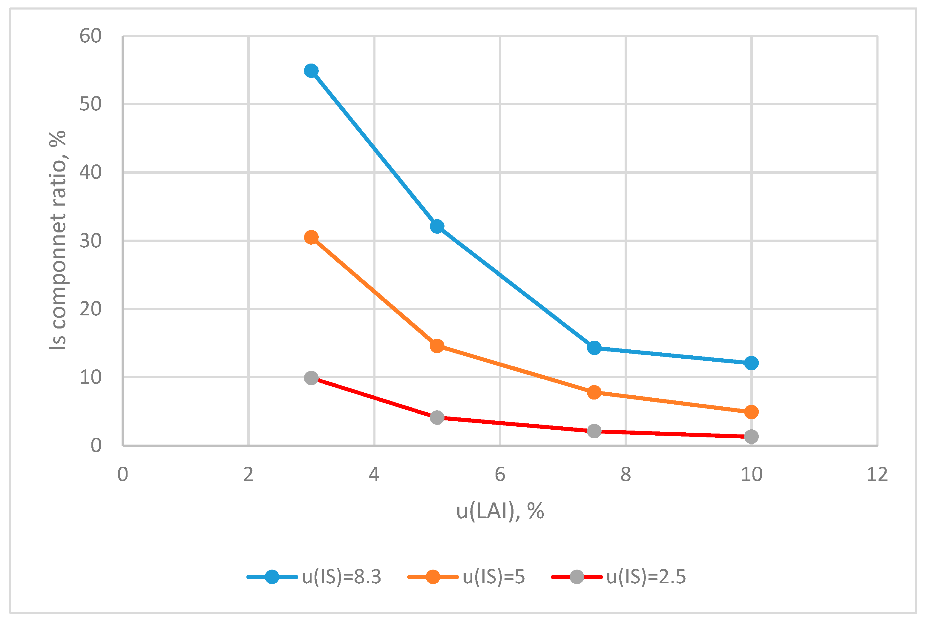
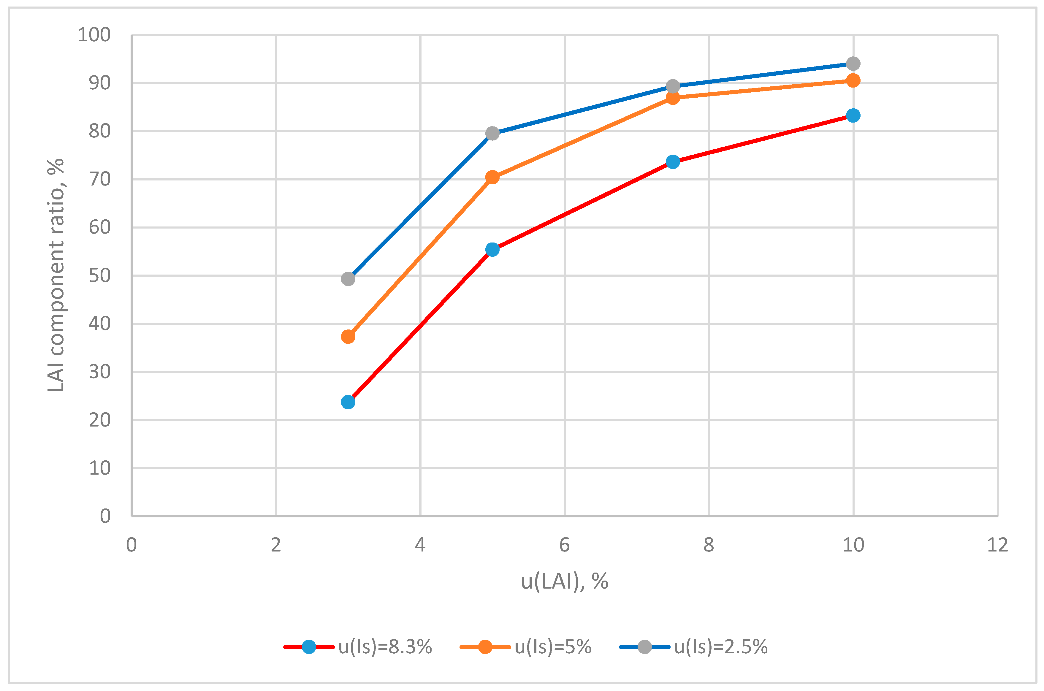
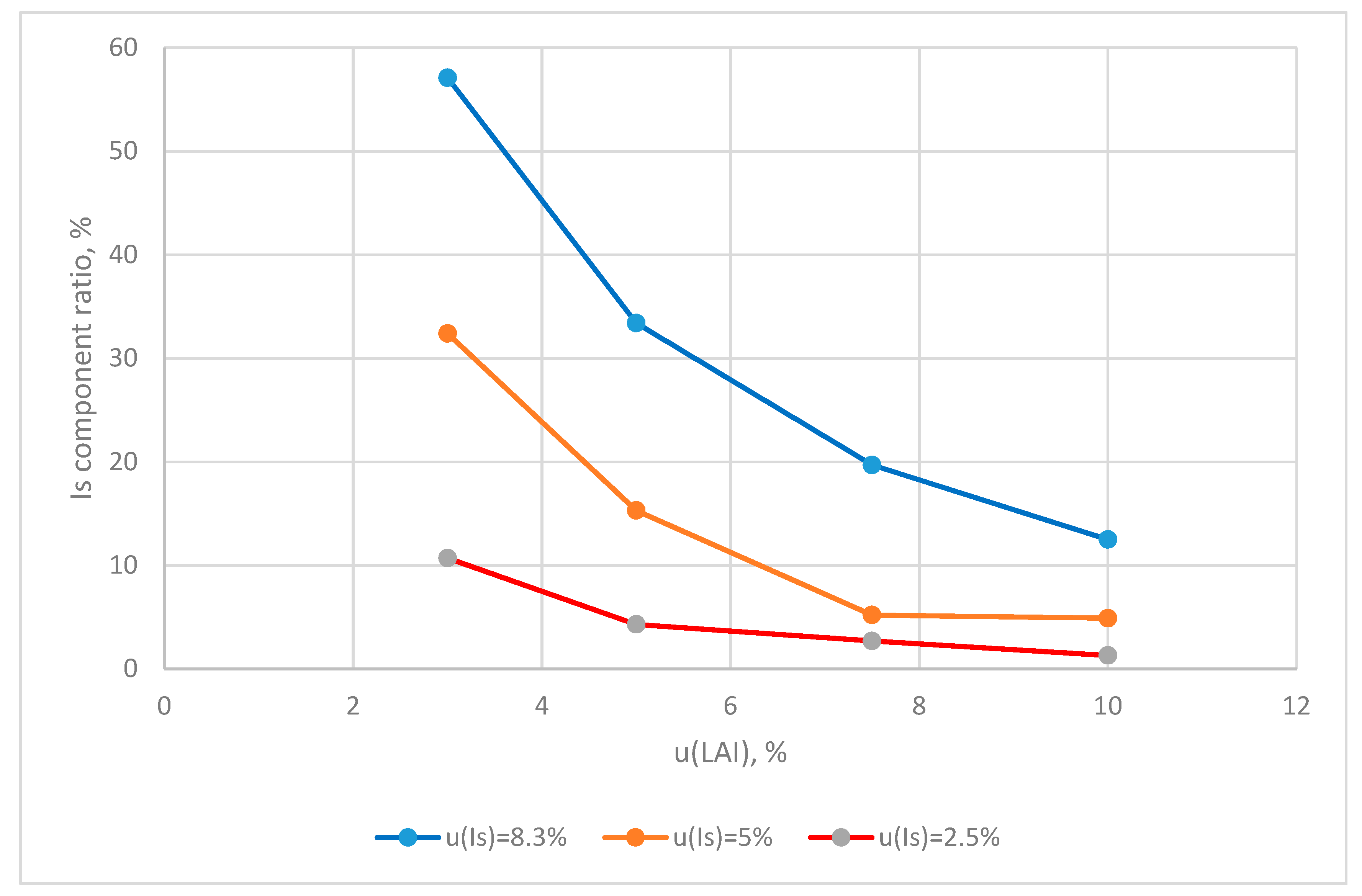
For the Stanghellini equation [6],

$$\partial \raisebox{1ex}{$({\mathrm{ET}}_{\mathrm{s}})$}\!\left/ \!\raisebox{-1ex}{$\partial \mathrm{LAI}$}\right.=\raisebox{1ex}{${\mathrm{K}}_1$}\!\left/ \!\raisebox{-1ex}{${\mathrm{K}}_3$}\right.\cdot {\mathrm{I}}_{\mathrm{s}}\cdot 0.7\left(\mathrm{Exp}(-0.7\mathrm{LAI}\right))+\raisebox{1ex}{${\mathrm{K}}_2$}\!\left/ \!\raisebox{-1ex}{${\mathrm{K}}_3$}\right.(1-\mathrm{RH})\mathrm{PVS}\cdot \mathrm{Uv}$$

(12)

$$\partial \raisebox{1ex}{${(\mathrm{ET}}_{\mathrm{s}})$}\!\left/ \!\raisebox{-1ex}{$\partial {\mathrm{I}}_{\mathrm{s}}$}\right.=\raisebox{1ex}{${\mathrm{K}}_1$}\!\left/ \!\raisebox{-1ex}{${\mathrm{K}}_3$}\right.(1-\mathrm{Exp}(-0.7\mathrm{LAI})$$

(13)

$$\raisebox{1ex}{$\partial {(\mathrm{ET}}_{\mathrm{s}})$}\!\left/ \!\raisebox{-1ex}{$\partial \mathrm{RH}$}\right.=-\raisebox{1ex}{${\mathrm{K}}_2$}\!\left/ \!\raisebox{-1ex}{${\mathrm{K}}_3$}\right.\mathrm{LAI}\cdot \mathrm{PVS}\cdot \mathrm{Uv}$$

(14)

$$\raisebox{1ex}{$\partial (E{T}_s)$}\!\left/ \!\raisebox{-1ex}{$\partial \mathrm{T}$}\right.=\raisebox{1ex}{${\mathrm{K}}_2$}\!\left/ \!\raisebox{-1ex}{${\mathrm{K}}_3$}\right.\cdot \mathrm{LAI}\cdot (1-\mathrm{RH})\cdot \mathrm{Uv}\cdot \left(1781.4\exp (\frac{17.2694}{\mathrm{T}+237.3})\right){\left(\frac{1}{\mathrm{T}+237.3}\right)}^2$$

(15)

$$\raisebox{1ex}{$\partial {(\mathrm{ET}}_{\mathrm{s}})$}\!\left/ \!\raisebox{-1ex}{$\partial \mathrm{Uv}$}\right.=\frac{\left[\mathrm{s}+\mathrm{r}\right]0.0096154\cdot \mathsf{\rho }\cdot {\mathrm{C}}_{\mathrm{p}}\cdot \mathrm{LAI}(1-\mathrm{RH})\mathrm{PVS}+0.0041346\mathrm{r}\cdot \mathrm{s}\cdot {\mathrm{r}}_{\mathrm{c}}\cdot {\mathrm{I}}_{\mathrm{s}}\left[1-\mathrm{Exp}(-0.7\mathrm{LAI})\right]}{{\left[\mathrm{s}+\mathrm{r}\left[1+0.3365\mathrm{Uv}\right]\right]}^2}.$$

(16)

For the Baille equation [12],

$${\mathrm{ET}}_{\mathrm{m}}=\mathrm{A}\cdot (1-\mathrm{Exp}\left[-0.7\mathrm{LAI}\right]{)\mathrm{I}}_{\mathrm{s}}+\mathrm{B}\cdot \mathrm{LAI}\cdot (1-\mathrm{RH})\cdot \mathrm{PVS}$$

(17)

$$\frac{\partial {(\mathrm{ET}}_{\mathrm{m}})}{\partial \mathrm{LAI}}=0.7\mathrm{A}\cdot (\mathrm{Exp}(-{0.7\mathrm{LAI}\left)\right)\mathrm{I}}_{\mathrm{s}}+\mathrm{B}\cdot (1-\mathrm{RH})\mathrm{PVS}$$

(18)

$$\frac{\partial {(\mathrm{ET}}_{\mathrm{m}})}{\partial {\mathrm{I}}_{\mathrm{s}}}=\mathrm{A}(1-\mathrm{Exp}(-0.7\mathrm{LAI}))$$

(19)

$$\frac{\partial {(\mathrm{ET}}_{\mathrm{m}})}{\partial \mathrm{RH}}=-\mathrm{B}\cdot \mathrm{LAI}\cdot \mathrm{PVS}$$

(20)

$$\frac{\partial {(\mathrm{ET}}_{\mathrm{m}})}{\partial \mathrm{T}}=\mathrm{B}\cdot (1-\mathrm{RH})\cdot 1781.4\mathrm{Exp}\left(\frac{17.2694\cdot \mathrm{T}}{\mathrm{T}+237.3}\right){\left(\frac{1}{\mathrm{T}+237.3}\right)}^2.$$

(21)

3. Results

Uncertainty Analysis of Two Evapotranspiration Models

The measurement values for calculating the model uncertainty were as follow:

T = 25 °C, RH = 40%, Is = 300 W/m², LAI = 2.2, Uv = 1.0 m/s.

The saturated vapor pressure (PVS) was 1.9695 kPa, VPD = 1.1803 kPa, the index of 1 − Exp (−0.7LAI)) was 0.7856. Only a sample of climate data was used in this case; the covariance items in Equation (10) were not considered.

The combined uncertainty for the Stanghellini model was calculated as follows:

$$\begin{gathered} {\mathrm{u}}^2{}_{\mathrm{C}}(\mathrm{ET})={\left(\frac{\partial {\mathrm{ET}}_{\mathrm{s}}}{\partial \mathrm{LAI}}\right)}^2{\mathrm{u}}^2(\mathrm{LAI})+{\left(\frac{\partial {\mathrm{ET}}_{\mathrm{s}}}{\partial \mathrm{Is}}\right)}^2{\mathrm{u}}^2\left(\mathrm{Is}\right)+ \\ {\left(\frac{\partial {(\mathrm{ET}}_{\mathrm{s}})}{\partial \mathrm{RH}}\right)}^2{\mathrm{u}}^2(\mathrm{RH})+{\left(\frac{\partial {\mathrm{ET}}_{\mathrm{s}}}{\partial \mathrm{T}}\right)}^2{\mathrm{u}}^2(\mathrm{T})+{\left(\frac{\partial {\mathrm{ET}}_{\mathrm{s}}}{\partial \mathrm{Uv}}\right)}^2{\mathrm{u}}^2(\mathrm{Uv}). \end{gathered}$$

(22)

The uncertainty of each variable is in

Table 3. The uncertainty of each variable.

Variable	Uncertainty	Source
LAI	u(LAI) = 0.22 (10%)	[21]
${\mathrm{I}}_{\mathrm{s}}$	u(Is) = 25 W/m2 (8.3%)	Manufacturer’s specification
T	u(T) = 0.37 °C	[37]
RH	u(RH) = 0.0165	[38]
Uv	$\mathrm{u}\left(\mathrm{Uv}\right)=0.08\raisebox{1ex}{$\mathrm{m}$}\!\left/ \!\raisebox{-1ex}{$\mathrm{s}$}\right.$	Manufacturer’s specification

.

The ET_s value was 4.624 g/m²-min, with uncertainty of u(ET_s) 0.389 g/m²-min. With the 95% significance level, the expanded value was 2.0. Therefore, the ET_s could be expressed as follows:

${\mathrm{ET}}_{\mathrm{s}}=4.624\pm 2\times 0.389$ = $4.624\pm 0.778$ g/m²-min.

The combined uncertainty for the Baille equation was calculated as follows:

$$\begin{gathered} {{\mathrm{u}}^2}_{\mathrm{C}}\left({\mathrm{ET}}_{\mathrm{m}}\right)={\left(\frac{\partial {\mathrm{ET}}_{\mathrm{m}}}{\partial \mathrm{LAI}}\right)}^2{\mathrm{u}}^2(\mathrm{LAI})+\left(\frac{\partial {\mathrm{ET}}_{\mathrm{m}}}{\partial \mathrm{Is}}\right){\mathrm{u}}^2(\mathrm{Is}) \\ +{\left(\frac{\partial {\mathrm{ET}}_{\mathrm{m}}}{\partial \mathrm{RH}}\right)}^2{\mathrm{u}}^2(\mathrm{RH})+{\left(\frac{\partial {\mathrm{ET}}_{\mathrm{m}}}{\partial \mathrm{T}}\right)}^2{\mathrm{u}}^2(\mathrm{T}). \end{gathered}$$

(23)

The calculating ET_m value was expressed as follows:

ET_m = 2.570$\pm 2\cdot 0.444$ = $2.570\pm 0.889$ g/m²-min.

The contribution of variable measurement to the uncertainties of the Stanghellini and Baille ET equations is in

Table 4. The contribution of variable measurement to uncertainty for the Stanghellini ET_s equation.

Variables	$\mathbf{Components}\left(\frac{\partial {\mathsf{\lambda }\mathbf{E}}_{\mathbf{T}}}{\partial {\mathbf{X}}_{\mathbf{i}}}\right)\mathbf{u}\left({\mathbf{X}}_{\mathbf{i}}\right)$ g/m2-min	Ratio Values %
LAI	453.13	83.20
${\mathrm{I}}_{\mathrm{s}}$	65.69	12.07
RH	24.58	4.52
T	0.843	0.15
Uv	0.143	0.06
${\mathrm{u}}^2{}_{\mathrm{c}}$	544.38	100%

and

Table 5. The contribution of variable measurement to uncertainty for the Baille ET_m equation.

Variable	$\mathbf{Components}\left(\frac{\partial {\mathsf{\lambda }\mathbf{E}}_{\mathbf{T}}}{\partial {\mathbf{X}}_{\mathbf{i}}}\right)\mathbf{u}\left({\mathbf{X}}_{\mathbf{i}}\right)$ g/m2-min	Ratio
LAI	147.40	83.23
${\mathrm{I}}_{\mathrm{s}}$	22.22	12.55
RH	07.22	4.08
T	0.26	0.14
${\mathrm{u}}^2{}_{\mathrm{c}}$	177.10	100%

. The uncertainty of the leaf area index (LAI) was the greatest factor in the ET uncertainty, representing 83.20% and 83.23% uncertainty in the Stanghellini and Baille equations, respectively. The uncertainty of Is was the second influencing factor, contributing 12.07% and 12.55% uncertainty to the Stanghellini and Baille equations, respectively.

The contribution of the RH measurement to uncertainty was the third influencing factor. The measurement range of temperature and wind velocity is 0–100 °C and 0–5 m/s, respectively. Considering the uncertainty of temperature and wind velocity (in Table 3) for the measuring range, the contribution of the temperature and wind velocity measurement to uncertainty only had a marginal effect.

The effect of the different u(LAI) and u(Is) values on the contribution ratio for LAI and Is in the Stanghellini equation is in Figure 1 and Figure 2.

The effect of two factors of the Baille equation is in Figure 3 and Figure 4.

With this observation, improving the performance of LAI and Is sensors was key to improving the ET equation. With reduced errors of LAI and Is sensors, the component ratio of uncertainty decreased significantly. Decreasing u(LAI) was more effective than decreasing u(Is) for reducing the ET uncertainty. With u(LAI) reduced to <5%, the contribution ratio of the LAI could be decreased significantly for two ET models. If the u(Is) was reduced to <5%, the same result of reducing uncertainty was found.

The effect of uncertainty of the LAI and Is on the uncertainty of the Stanghellini and Baille models is in

Table 6. The effect of uncertainty of the leaf area index (LAI) and solar intensity (I_s) in the uncertainty analysis for the Stanghellini ET_s equation.

U (Is)	U (LAI), g/m2-min
	10%	7.5%	5.0%	2.5%
8.3%	0.389	0.310	0.234	0.161
5.0%	0.374	0.291	0.213	0.147
2.5%	0.367	0.282	0.201	0.129

and

Table 7. The effect of uncertainty of the leaf area index (LAI) and solar intensity (I_s) in the uncertainty analysis for the Baille ET_m equation.

U (Is)	U (LAI), g/m2-min
	10%	7.5%	5.0%	2.5%
8.3%	0.222	0.177	0.136	0.104
5.0%	0.213	0.165	0.121	0.083
2.5%	0.209	0.160	0.114	0.072

. With the largest errors, u(LAI) = 10% and u(I_s) = 8.3%, the largest uncertainty was 0.389 g/m²-min and 0.222 g/m²-min, respectively.

With u(LAI) reduced to 0.11 (5%) and $\mathrm{u}\left(\mathrm{Is}\right)$ to 5 W/m² (5%), the combined uncertainty of ET_s and ET_m was 0.213 g/m²-min and 0.121 g/m²-min for the Stanghellini and Baille equations, respectively. If the performance of sensors could be improved, u(LAI) was reduced to 0.055 (2.5%) and $\mathrm{u}\left(\mathrm{Is}\right)$ was reduced to 2.5 W/m² (2.5%), for combined uncertainty of ET_s and ET_m 0.122 g/m²-min and 0.072 g/m²-min for the Stanghellini and Baille equations, respectively. ET_s and ET_m uncertainty reduced significantly with the improved sensor performance.

4. Discussion

In the biological model, the relationship between specific variables and influencing factors of biological systems can be expressed with mathematical formulas. The difference between predicted value and actual value of the model is called an error. Error sources include instrumental errors, sampling errors, spatial and temporal errors, and other factors. The effect of these error sources on the combined uncertainties need to be evaluated. The uncertainty component of LAI was the greatest factor in the uncertainty component of the two ET models. Simic et al. [39] mentioned the importance of the LAI value in the ET calculation. Kumar et al. [40] emphasized the quality of meteorological data to calculate ET values. Villarreal-Guerrero et al. [22] considered the high sensitivity of the LAI and Is sensors in the validation of ET models. The results of this study confirmed the conclusions.

Our results indicate the importance of sensor performance. The measurement uncertainty of the LAI meter is due to measurement error and inadequate sampling. This uncertainty could be reduced with the calibration technique and training in operation [41].

There are two methods to measure the LAI value, indirect and direct [42,43]. The indirect method is to use an instrument, such as digital hemispherical photography, and the LI-COR LAI-2000 Plant Canopy Analyzer. The performance improvement of these instruments is related to its manufacturers. The direct method is to measure the leaf area within a specific area and calculate LAI values with the calibration equations [44,45]. With adequate calibration equations, the calculated LAI values were close to actual LAI values [42,43]. This provides a way to improve the measurement of LAI values and reduce its measurement uncertainty.

The sources of measurement uncertainty of the Is meter include absolute error from the manufacturer, spectral response error, tilt error, linearity error, temperature effect error, and user error [46]. These error components could be improved by calibration with the primary standard Pyranometer and adequate operation of sensors. Myers et al. [47] described a detailed calibration procedure to reduce the uncertainty of a Pyranometer, ranging from 2.5% to 3.0%.

The uncertainty of the RH measurement is the third influencing factor. These electrical sensors could be calibrated with several kinds of saturated salt solutions [38].

The results of this study indicated that the humidity and wind velocity have very low influence in the greenhouse ET model. These results confirm the possibility to simplify the ET model, as suggested by Carmassi et al. [48], Marfa et al. [49] and Bacci et al. [50].

In this study, we evaluated the effect of the u(LAI), u(Is), u(T), u(RH), and u(Uv) on the contribution ratio for ET models calculated by the ISO method. Cooman and Schrevens [51] used a sensitivity analysis to analyze the effect of temperature, CO₂, and Is on the predictive ability of the tomato growth model. The effect of each environmental factor was compared with simulation results directly. In this study, the measurement performance of environment sensors was quantified, so the uncertainty analysis could provide more information than sensitivity analysis for model evaluation.

With the conditions of the largest errors, u(LAI) = 10% and u(Is) = 8.3%, the largest uncertainty was 0.389 g/m²-min and 0.222 g/m²-min for the Stanghellini and Baille ET models, respectively. Boulard and Wang [21] indicated that the standard deviation of the linear regression between calculated and measurement ET values was 0.153 g/m²-min to 0.388 g/m²-min. The difference between actual and calculated ET values found in the literature ranged from 0 to 3.98 g/m²-min. [21,22,23]. Thus, the uncertainty of the ET models from the sensor performance cannot be neglected in validating ET models.

The actual ET values are measured using a lysimeter or other methods [34]. The uncertainty of each measurement method may be the uncertainty source in the model. For example, the error of the balance was 1g in the study of Medrano et al. [12]. The detailed information of ET reports was introduced by Allen et al. [34]. Ten ET measurement methods and anticipated errors were discussed. The error with the lysimeter method typically ranged from 5% to 15%. The importance of the measurement quality of weather data was also emphasized by Allen et al. [35]. These factors could be incorporated into the uncertainty analysis proposed in this study.

Villarreal-Guerreroa et al. [22] mentioned that crop resistance may be a limitation for ET prediction. In this study, the value for each parameter was adopted from the literature. The numeric value of these parameters may be the source of uncertainty. Further studies will be needed to study the effect of uncertainty of these parameters on the ET equation. Brugnach et al. [26] mentioned the uncertainty sources of the biological model, which are the measurement of variables, the correction of the utilization values of parameters, the sampling technique of the biological activity, and the concept of models. In this study, the assumption of two ET models is the energy translation between sensible and latent heat. The assumption of the ET model may be a source of uncertainty. In the modelling transpiration of greenhouse gerbera (Gerbera jamesonii H. Bolus) grown in substrate, NaCl salinity was found to have a significant effect on ET values [52].

In this brief report, the measurement uncertainty of the biological environment model was expressed with the ISO GUM concept. Only one sample of climate data was used to evaluate the effect of environmental measurement uncertainty on prediction of evapotranspiration, and the interaction of variables was not considered in this study. Future studies will be performed to evaluate more influencing factors. The effect of the measurement accuracy of variables and the interaction of these variables on the measurement uncertainty of ET values will need to be evaluated.

We used two typical ET models to evaluate uncertainty by the ISO concept and method. Other ET models could be evaluated with the same procedures.

5. Conclusions

In this study, two simple forms of ET models of tomato in a greenhouse were used to evaluate the effect of environmental measurement uncertainty on the prediction of evapotranspiration. The solar radiation and vapor pressure deficit have a significant effect on ET values. Solar radiation was the dominating factor. The concept and method of the ISO GUM was adopted. The performance of the leaf area index (LAI) and solar radiation (Is) sensors were the main factors. At the conditions of u(LAI) = 10% and u(Is) = 8.3%, the uncertainty was 0.389 g/m²-min and 0.222 g/m²-min for the Stanghellini and Baille ET models, respectively. The performance of these sensors needed to be improved to ensure the predictive ability for applying the ET model for irrigation management of crops. The method proposed in this study can be used for the uncertainty evaluation of ET models that calculate ET based on environmental variables measured by meteorological sensors or the remote sensing technique. The effect of the measurement accuracy of variables of other influencing factors needs to be evaluated.

References

1. Doorenbos, J.; Pruitt, W.O. Guidelines for Predicting Crop Water Requirements; Food and Agriculture Organisation: Rome, Italy, 1977. [Google Scholar]
2. Ilahi, W.F.F. Evapotranspiration Models in Greenhouse. Master’s Thesis, Wageningen University, Wageningen, The Netherlands, 2009. [Google Scholar]
3. Luoa, C.; Wanga, Z.; Sauer, T.J.; Helmers, M.J.; Hortona, R. Portable canopy chamber measurements of evapotranspiration in corn, soybean, and reconstructed prairie. Agric. Water Manag. 2018, 198, 1–9. [Google Scholar] [CrossRef] [Green Version]
4. Maes, W.H.; Steppe, K. Estimating evapotranspiration and drought stress with ground-based thermal remote sensing in agriculture: A review. J. Exp. Bot. 2012, 63, 4671–4712. [Google Scholar] [CrossRef] [PubMed]
5. Feng, Y.; Burian, S.J.; Pardyjak, E.R. Observation and estimation of evapotranspiration from an irrigated green roof in a rain-scarce snvironment. Water 2018, 10, 262. [Google Scholar] [CrossRef]
6. Stanghellini, C. Transpiration of Greenhouse Crops an Aid to Climate Management. Ph.D. Thesis, Agricultural University, Wageningen, The Netherlands, 1987. [Google Scholar]
7. Bailey, B.J.; Montero, J.I.; Blel, C.; Wilkinson, D.J.; Anton, A.; Jolhet, O. Transpiration of Ficus benjamina: Comparison of measurements with predictions of the Penman–Monteith model and a simplified version. Agric. For. Meteorol. 1993, 65, 229–243. [Google Scholar] [CrossRef]
8. Baille, M.; Baille, A.; Laury, J.C. A simplified model for predicting evapotranspiration rate of nine ornamental species vs climate factors and leaf area. Sci. Hortic. 1994, 59, 217–232. [Google Scholar] [CrossRef]
9. Baille, M.; Baille, A.; Laury, J.C. Canopy surface resistances to water vapour transfer for nine greenhouse pot plant crops. Sci. Hortic. 1994, 57, 143–155. [Google Scholar] [CrossRef]
10. Seginer, I. The Penman–Monteith evapotranspiration equation as an element in greenhouse ventilation design. Biosyst. Eng. 2002, 82, 423–439. [Google Scholar] [CrossRef]
11. Rouphael, Y.; Colla, G. Modelling the transpiration of a greenhouse zucchini crop grown under a Mediterranean climate using the Penman–Monteith equation and its simplified version. Aust. J. Agric. Res. 2004, 55, 931–937. [Google Scholar] [CrossRef]
12. Medrano, E.; Lorenzo, P.; Sa´nchez-Guerrero, M.C.; Montero, J.I. Evaluation and modelling of greenhouse cucumber-crop transpiration under high and low radiation conditions. Sci. Hortic. 2005, 105, 163–175. [Google Scholar] [CrossRef]
13. Irmak, A. Evapotranspiration—Remote Sensing and Modeling; INTECH open Access Publisher: London, UK, 2011. [Google Scholar]
14. Gerosa, G. Evapotranspiration—From Measurements to Agricultural and Environmental Applications; INTECH open Access Publisher: London, UK, 2011. [Google Scholar]
15. Wang, K.; Dickinson, R.E. A review of global terrestrial evapotranspiration: Observation, modeling, climatology, and climatic variability. Rev. Geophys. 2012, 50, RG2005. [Google Scholar] [CrossRef]
16. Xiao, W.; Wei, Z.; Wen, X. Evapotranspiration partitioning at the ecosystem scale using the stable isotope method—A review. Agrc. For. Meteorol. 2018, 263, 346–361. [Google Scholar] [CrossRef]
17. Knighton, J.; Saia, S.M.; Morris, C.K.; Archiblad, J.A.; Walter, M.T. Ecohydrologic considerations for modeling of stable water isotopes in a small intermittent watershed. Hydrol. Process. 2017, 31, 2438–2452. [Google Scholar] [CrossRef]
18. Ivezic, V.; Bekic, D.; Horvat, B. Modelling of basin wide daily evapotranspiration with a partial integration of remote sensing data. Atmosphere 2018, 9, 120. [Google Scholar] [CrossRef]
19. Martano, P. Evapotranspiration estimates over non-homogeneous mediterranean land cover by a calibrated “critical resistance” approach. Atmosphere 2015, 6, 255–272. [Google Scholar] [CrossRef]
20. Zhao, P.; Lüers, J. Parameterization of evapotranspiration estimation for two typical East Asian crops. Atmosphere 2017, 8, 111. [Google Scholar] [CrossRef]
21. Boulard, T.; Wang, S. Greenhouse crop transpiration simulation from external climate conditions. Agric. For. Meteorol. 2000, 100, 25–34. [Google Scholar] [CrossRef]
22. Villarreal-Guerreroa, F.; Kaciraa, F.M.; Fitz-Rodrigueza, E.; Kubotab, C.; Giacomellia, G.A.; Linkerc, R.; Arbeld, A. Comparison of three evapotranspiration models for a greenhouse cooling strategy with natural ventilation and variable high pressure fogging. Sci. Hortic. 2012, 134, 210–221. [Google Scholar] [CrossRef]
23. Hamby, D.M. A review of techniques for parameter sensitivity analysis of environmental models. Environ. Monit. Assess. 1994, 32, 135–154. [Google Scholar] [CrossRef] [PubMed] [Green Version]
24. Moriasi, D.N.; Arnold, J.G.; van Liew, M.W.; Bingner, R.L.; Harmel, R.D.; Veith, T. Model evaluation guidelines for systematic quantification of accuracy in watershed simulations. Trans. ASABE 2007, 50, 885–900. [Google Scholar] [CrossRef]
25. Van Gadow, K.; Hui, G. Modelling Forest Development; Kluwer Academic Publishers: Boston, MA, USA, 1999. [Google Scholar]
26. Brugnach, M.; Pahl-Wostl, C.; Lindenschmidt, K.E.; Janssen, J.A.E.B.; Filatova, T.; Mouton, A.; Holtz, G.; van der Keur, P.; Gaber, N. Complexity and uncertainty: Rethinking the modelling activity. Dev. Int. Environ. Assess. 2008, 3, 49–68. [Google Scholar]
27. ISO; BIMP; IEC; IFCC; IUPAC; IUPAP; OIML. Guide to the Expression of Uncertainty in Measurement; ISO: Geneva, Switzerland, 1993. [Google Scholar]
28. ISO/IEC 98-3. Uncertainty of Measurement—Part 3: Guide to the Expression of Uncertainty in Measurement; ISO: Geneva, Switzerland, 2010. [Google Scholar]
29. Crout, N.; Kokkonen, T.; Jakeman, A.J.; Norton, J.P.; Newham, L.T.H.; Anderson, R.; Assaf, H.; Croke, B.F.W.; Gaber, N.; Gibbons, J.; et al. Good modelling practice. Dev. Int. Environ. Assess. 2008, 3, 15–31. [Google Scholar]
30. Larocque, G.R.; Bhatti, J.S.; Gordon, A.M.; Luckai, N.; Wattenba, M.; Liu, J.; Peng, C.; Arp, P.A.; Liu, S.; Zhang, C.F.; et al. Uncertainty and sensitivity issues in process-based models of carbon and nitrogen cycles in terrestrial ecosystems. Dev. Inte. Environ. Assess. 2008, 3, 307–327. [Google Scholar]
31. ASHRAE. Brochure on psychrometry. American Society of Heating, Refrigerating, and Air; Conditioning Engineers: Atlanta, GA, USA, 1977. [Google Scholar]
32. Picard, A.; Davis, R.; Glaser, M.; Fuji, K. Revised formula for the density of moist air (CIPM-2007). Metrologia 2006, 45, 149–155. [Google Scholar] [CrossRef]
33. Albright, L.D. Psychometrics. Environmental Control for Animals and Plants; The American Society of Agricultural Engineers: Joseph, MI, USA, 1990. [Google Scholar]
34. Allen, R.G.; Pereira, L.S.; Howell, A.; Jensen, M.E. Evapotranspiration information reporting: I. Factors governing measurement accuracy. Agric. Water Manag. 2011, 98, 899–920. [Google Scholar] [CrossRef]
35. Allen, R.G.; Pereira, L.S.; Howell, A.; Jensen, M.E. Evapotranspiration information reporting: II. Recommended documentation. Agric. Water Manag. 2011, 98, 921–929. [Google Scholar] [CrossRef]
36. Tahiri, A.; Anyoji, H.; Yasuda, H. Fixed and variable light extinction coefficients for estimating plant transpiration and soil evaporation under irrigated maize. Agric. Water Manag. 2006, 84, 186–192. [Google Scholar] [CrossRef]
37. Chen, C. Evaluation of measurement uncertainty for thermometers with calibration equations. Accredit. Qual. Assur. 2006, 11, 75–82. [Google Scholar] [CrossRef] [Green Version]
38. Lu, H.; Chen, C. Uncertainty evaluation of humidity sensors calibrated by saturated salt solutions. Measurement 2007, 40, 591–599. [Google Scholar] [CrossRef]
39. Simic, A.; Fernandes, R.; Wang, S. Assessing the impact of leaf area index on evapotranspiration and groundwater recharge across a shallow water region for diverse land cover and soil properties. J. Water Res. Hydraul. Eng. 2017, 3, 60–73. [Google Scholar]
40. Kumar, R.; Shankar, V.; Kumar, M. Modelling of crop reference evapotranspiration: A review. Universal J. Environ. Res. Technol. 2001, 1, 239–246. [Google Scholar]
41. Dovey, S.B.; du Toit, B. Calibration of LAI-2000 canopy analyser with leaf area index in a young eucalypt stand. Trees 2006, 20, 273–277. [Google Scholar] [CrossRef]
42. Bread, N.J.J. Ground-based measurements of leaf area index: A review of methods, instruments and current controversies. J. Exp. Bot. 2013, 54, 2403–2417. [Google Scholar] [CrossRef] [PubMed]
43. Olivas, P.C.; Steven, F.; Oberbauer, D.B.; Clark, D.A.; Clark, M.G.; Ryan, M.G.; O’Brien, J.J.; Ordoñez, H. Comparison of direct and indirect methods for assessing leaf area index across a tropical rain forest landscape. Agric. Meteorol. 2013, 177, 110–116. [Google Scholar] [CrossRef]
44. Blanco, F.F.; Folegatti, M.V. A new method for estimating the leaf area index of cucumber and tomato plants. Hortic. Bras. 2003, 21, 666–669. [Google Scholar] [CrossRef] [Green Version]
45. Carmassi, G.; Incrocci, L.; Incrocci, G.; Pardossi, A. Non-destructive estimation of leaf area in (Solanum lycopersicum L.) and gerbera (Gerbera jamesonii H. Bolus). Agric. Mediterr. 2007, 137, 172–176. [Google Scholar]
46. Vignola, F.; Joseph Michalsky, J.; Stoffel, T. Solar and Infrared Radiation Measurements; CRC Press: Boca Raton, FL, USA, 2012. [Google Scholar]
47. Myers, D.R.; Stoffel, T.L.; Reda, I.; Wicoz, S.M.; Andreas, A.M. Recent progress in reducing the uncertainty in and improving Pyranometer calibrations. Trans. ASME 2002, 124, 44–50. [Google Scholar] [CrossRef]
48. Carmassi, G.; Incrocci, L.; Maggini, R.; Malorgio, F.; Tognoni, F.; Pardossi, A. An aggregated model for water requirements of greenhouse tomato grown in closed rockwool culture with saline water. Agric. Water Manag. 2007, 88, 73–82. [Google Scholar] [CrossRef]
49. Marfà, O.; Biel, C.; Blanch, F.; Montero, J.I. Water consumption of a closed soilless culture of gerbera: Usefulness of model to estimate evapotranspiration. Acta. Hortic. 2000, 534, 147–153. [Google Scholar] [CrossRef]
50. Bacci, L.; Battista, P.; Cardarelli, M.; Carmassi, G.; Rouphael, Y.; Incrocci, L.; Malorgio, F.; Pardossi, A.; Rapi, B.; Colla, G. Modelling Evapotranspiration of Container Crops for Irrigation Scheduling. In Evapotranspiration-From Measurements to Agricultural and Environmental Applications; InTech Open Access Publisher: London, UK, 2011. [Google Scholar] [Green Version]
51. Cooman, A.; Schrevens, E. Sensitivity of the Tomgro model of solar radiation intensity, air temperature and carbon dioxide concentration. Biosyst. Eng. 2007, 96, 249–255. [Google Scholar] [CrossRef]
52. Carmassi, G.; Bacci, L.; Bronzini, M.; Incrocci, L.; Maggini, R.; Bellocchi, G.; Massa, D.; Pardossi, A. Modelling transpiration of greenhouse gerbera (Gerbera jamesonii H. Bolus) grown in substrate with saline water in a Mediterranean. Sci. Hortic. 2013, 156, 9–18. [Google Scholar] [CrossRef]
Figure 1. The effect of u(LAI) and u(Is) on the lead area index (LAI) contribution ratio for the Stanghellini equation.
Atmosphere 09 00400 g001
Figure 2. The effect of u(LAI) and u(Is) on the solar radiation (Is) contribution ratio for the Stanghellini equation.
Atmosphere 09 00400 g002
Figure 3. The effect of u(LAI) and u(Is) on the LAI contribution ratio for the Baille equation.
Atmosphere 09 00400 g003
Figure 4. The effect of u(LAI) and u(Is) on the Is contribution ratio for the Baille equation.
Atmosphere 09 00400 g004