Article

Horizontal Electric Field in the Vicinity of Structures Hit by Lightning

by
Celio Fonseca Barbosa
Converging Networks Department, Fundacao CPqD, 13086-902 São Paulo, Brazil
Atmosphere 2016, 7(9), 115; https://doi.org/10.3390/atmos7090115
Submission received: 24 August 2016 / Revised: 3 September 2016 / Accepted: 5 September 2016 / Published: 9 September 2016

Abstract

:
The horizontal electric field at the ground surface in the vicinity of structures hit by lightning flashes is relevant to the safety of human beings and livestock; it determines the touch and step voltages around the structure. This paper uses an approximate analytical formula for calculating the horizontal electric field, which was adapted to take into account the effect of the structure foundation. The input for the calculation is the current waveform at the base of the structure, and the results agree well with those obtained by other authors using the finite-difference time-domain (FDTD) method. The approximate formula is applied to calculate touch and step voltages in the vicinity of a structure and the results show that the use of the direct current (DC) approximation to calculate touch and step voltages may lead to significant errors; especially for fast-rising currents and relatively good-conducting soils. This means that DC approximation could be used for positive first stroke and poor-conducting ground (ρ ≥ 1000 Ω∙m), but cannot be used for subsequent strokes and good-conducting ground (ρ ≤ 100 Ω∙m). Moreover, step voltages differ more from the DC approximation than the touch voltages.

1. Introduction

The horizontal electric field at the ground surface in the vicinity of structures hit by lightning flashes is relevant to the safety of human beings and livestock, as it determines the touch and step voltages around the structure. This is recognized by the international standard on lightning protection [1], which provides requirements to protect people around structures against touch and step voltages. For instance, the standard requires a 100 kV impulse withstand level (at 1.2/50 μs) for lightning down-conductor insulation in order to provide protection against touch voltages.
The assessment of step and touch voltages due to lightning is often carried out using direct-current (DC) techniques, which neglects the electric field components induced by the time-varying return stroke current and its propagation effects. The rigorous solution to this problem can be carried out using numerical methods, such as finite-difference time-domain (FDTD) [2]. Although numerical methods provide reliable results, they have the drawback of requiring detailed modeling of the real installation, which has to be carried out by skilled personnel using significant computational resources and specialized software.
On the other hand, the analytical calculation of the electromagnetic fields for the canonical problem of a vertical conductor carrying alternating current into lossy ground has been demonstrated by Sommerfeld [3] about one century ago. Sommerfeld’s solution is described in detail in [4] and it is expressed in terms of a series of slow-converging integrals that were almost impossible to be rigorously computed at that time. It was only after the development of digital computers that efficient numerical computation of Sommerfeld integrals was possible. Zeddam [5] was the first to apply Sommerfeld integrals to the calculation of lightning electromagnetic fields considering lossy ground and, in particular, to the calculation of the horizontal electric field due to lightning. As Sommerfeld’s solution is in the frequency domain, its use for the calculation of lightning electromagnetic fields requires that the calculation is carried out at a large number of frequencies, so that the time-domain solution can be obtained from Fourier transforms. Lately, other authors have developed efficient methods to compute Sommerfeld integrals in lightning-related problems [6,7,8,9,10,11], which reduce significantly the computational resources required.
Cooray [12] provided a method for calculating the lightning horizontal electric field at the ground surface by multiplying the azimuthal magnetic field to the surface impedance, leading to a simple and reasonably accurate expression. This expression was later complemented by Rubinstein [13] by adding an aerial component, resulting in the so-called Cooray-Rubinstein formula that is widely used in the calculation of lightning induced voltages in overhead lines [14,15]. However, the surface impedance approximation provides accurate results only if the point of interest is relatively far from the lightning channel base. This issue has been investigated by Cooray [16], who concluded that the surface impedance approximation can generate a correct horizontal electric field when the distance to the point of interest is larger than about 50, 200, and 500 m for ground resistivity values of 100, 1000, and 10,000 Ω∙m, respectively. Therefore, the surface impedance formulation cannot be used for step and touch voltage assessment, as in this case the point of interest is usually close to the lightning current (channel base or structure base).
Barbosa and Paulino [17] developed an approximate time-domain expression for the horizontal electric field from lightning, which provides results that are equivalent to those from the Cooray-Rubinstein formula. The main advantage of a time-domain solution is that it does not require the domain translation by means of Fourier transforms, making the calculation process straightforward. This characteristic is particularly useful when assessing the indirect lightning performance of overhead lines [18,19]. Lately, other authors have also developed time-domain solutions to this problem [20,21,22]. However, these solutions are all limited to regions relatively far from the lightning current, so they cannot be applied to the vicinity of a structure hit by lightning.
An approximate expression for the lightning horizontal electric field that can be applied in the vicinity of the lightning striking point was developed by Barbosa and Paulino [23] by adding a late-time constant in their previous formula. The resulting expression was validated by comparing its results with those obtained by Cooray [24] using Sommerfeld integrals. Recently, Cooray [16] successfully applied the expression from [23], together with an attenuation function, in order to calculate the underground horizontal electric field due to lightning.
Therefore, the approximate expression developed by Barbosa and Paulino can be used to compute the lightning horizontal electric field at close and far ranges [25,26,27]. However, its application to the case of a structure hit by lightning faces two problems: (i) The expression was developed considering that the return stroke current starts at ground level, whereas in this case it starts at the top of the structure; (ii) The late time response was based on the assumption of symmetric current distribution from the bottom of the lightning channel, whereas in this case it is likely to be influenced by the structure foundation and its associated grounding system.
This paper investigates these issues and proposes an amendment to the original expression in order to take into account the effect of the structure foundation in the nearby horizontal electric field. The resulting expression is a straightforward tool to compute step and touch voltages in the vicinity of structures hit by lightning. The paper is organized as follows. In Section 2, some theoretical considerations are provided in order to justify the use of the approximate expression for the horizontal electric field calculation in the case of a strike to a structure, and to propose an amendment to take into account the effect of the structure foundation. Section 3 presents calculation results obtained with the approximate expression and compares them with those obtained by Baba and Rakov [2] using FDTD. Section 4 applies the method in the assessment of touch and step voltages using the standard lightning current waveforms [28] and compares the results with those obtained with DC approximation, in order to highlight the conditions that allow or prevent the use of the latter. Finally, Section 5 discusses some relevant aspects of the approximations considered and Section 6 draws the main conclusions.

2. Theoretical Considerations

2.1. Effect of Placing the Channel Base on the Top of the Structure

As mentioned in the Introduction, Barbosa and Paulino [23] developed their expression considering that the return stroke starts at ground level, which is the usual assumption. However, in the present case the return stroke starts from the top of the structure, resulting in two current waves: one propagating downward towards the ground and the other propagating upwards towards the thunderclouds. It is then necessary to assess the implication of this fact on the formulation.
Let us first consider the original situation, where the return stroke starts at ground level and an observer is also standing on the ground at a distance x from the channel base, as shown in Figure 1a. The ground is considered as perfectly conducting, the stroke current propagates with the velocity of light in free space (c), and the return stroke current has a step waveform. The current propagation is not subjected to attenuation nor distortion, according to the transmission line (TL) model [29]. According to Rusck [30], after t0 = x / c, the observer will “see” a step magnetic field with amplitude:
H 0 = I 0 2 π x
which means that he receives the full magnetic field, although at t0 the stroke current is yet at a height x from the ground surface. This outcome is also in line with Cooray and Cooray [31], who demonstrated that an electric charge accelerated to the velocity of light radiates electromagnetic energy only at the bottom of the channel, i.e., where it is under acceleration. Of course, if the charge is decelerated at some point along the channel, it would also radiate electromagnetic energy.
Let us now consider the situation shown in Figure 1b, where the return stroke starts at the top of a vertical structure of height h. As the structure is surrounded by air, it is assumed that the current propagation velocity is c. Furthermore, the structure is modeled as a uniform and lossless transmission line. In this figure, the return stroke inception is represented by negative charges flowing downward and positive charges flowing upward, as would be expected from a negative flash. The resulting spherical wave propagates outward from the channel base. Choosing the magnetic field to track the wave front, it is clear in Figure 1b that it wanes when propagating radially, but does not wane when propagating vertically. Therefore, the observer will "see" the step magnetic field given by Equation (1), i.e., as if the return stroke had started from ground level. The only difference is that, in this case, the time taken for the wave to reach the observer is:
t 0 = h 2 + x 2 c
If it is assumed that the current propagates at the speed of light in both the lightning channel and the structure, the field wave is produced only at the attachment point, resulting in a spherical field wave that moves outward from this point. However, the lightning channel usually has higher impedance and lower propagation velocity than the structure. For a point at ground level close to the structure, the most relevant contribution of the lightning channel to the horizontal electric field is the reflection of the current wave at the structure/channel transition. Indeed, the original downward current reflects at ground level and moves upward, when it reflects again at the bottom of the channel and so on. In real life, the travelling current in the structure vanishes fast due to the losses in the process. Furthermore, the impedance of the structure is usually lossy and non-uniform, so that the current is expected to experience some degree of attenuation and distortion as it propagates.
It is interesting to have a closer look at the bottom of the structure shown in Figure 1b at the time when the step downward current wave arrives. An observer at this point will “see” a magnetic field wave composed of a single step of amplitude 2 H0, due to the full current reflection at perfectly conducting ground. However, an observer at distance x will “see” two consecutive magnetic field steps of amplitude H0 superimposed: one excited at the structure top and that arrives at the instant given by (2) and another excited at the structure base and that arrives at:
t 1 = h + x c
Of course, for an observer placed relatively close to the structure (x << h), this time difference is negligible. This is the case for the assessment of touch and step voltages. For instance, for h = 160 m and x = 15 m, the time delay between the two consecutive magnetic field steps is only 0.05 μs. However, this effect becomes more relevant as the observer moves away from the structure.
Therefore, it comes out that the knowledge of the current flowing at the structure base is sufficient for the calculation of the horizontal electric field at the ground surface in the vicinity of a structure hit by lightning. As a consequence, the expressions originally developed for the return stroke starting at ground level could be applied to the case where the return stroke starts at the top of the structure. The validity of this approach will be verified in Section 3.

2.2. Effect of the Structure Foundation
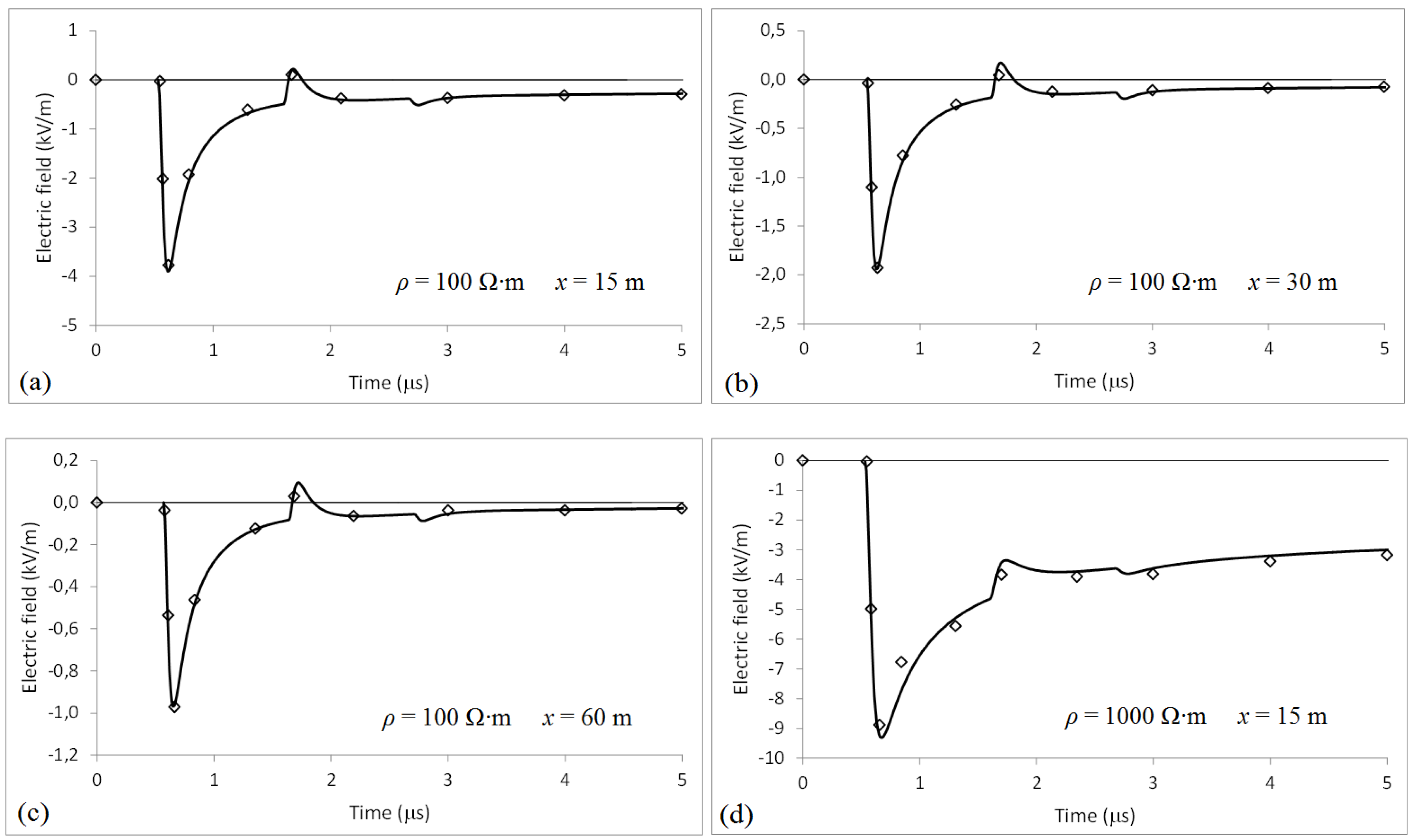
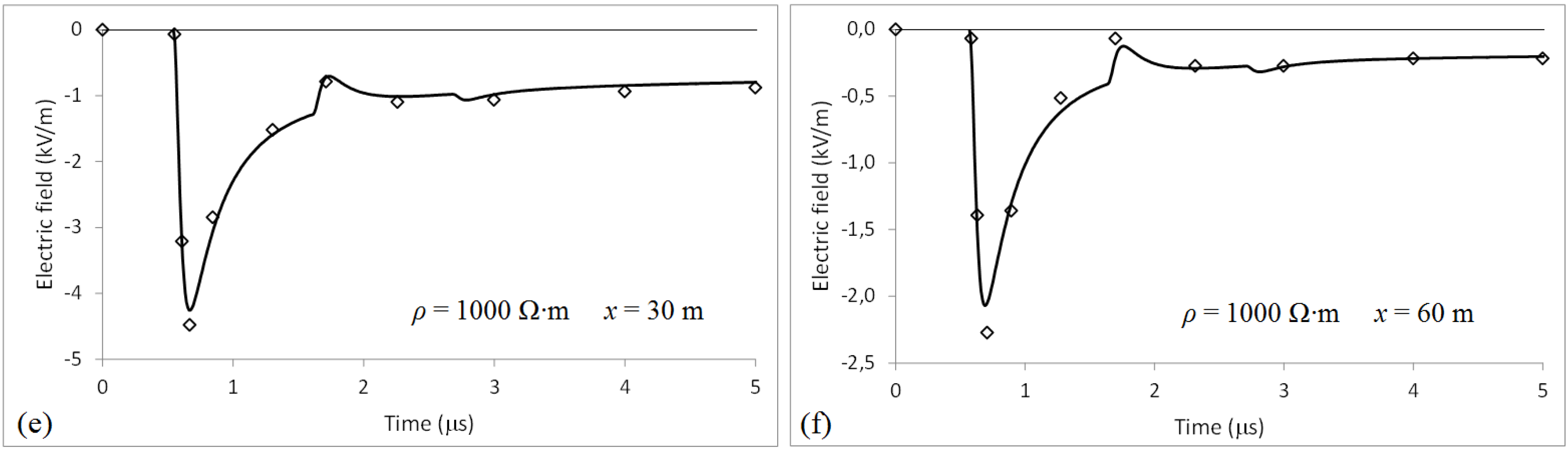
The horizontal electric field at ground level in the vicinity of a structure is affected by the dimensions and shape of the structure foundation. As the distance from the structure increases, the late-time ground current density attains radial symmetry and the electric field becomes progressively independent of the structure foundation. In the modeling proposed by Barbosa and Paulino [23], no foundation was considered, so that the late-time ground current density was assumed as radially symmetrical from the point that the current enters the ground. In order to take into account the effect of the structure foundation in the nearby electric field, a modification is introduced in the electric field expression, as described in the following.
Considering a step magnetic field wave H0 reaching a point at the ground surface, the resulting horizontal electric field according to [23] reads:
E H = Z E H 0 { 2 ε R + a t ( 1 + 3 b ε R + 2 a b t ) 2 ( 1 + a b t ) 1 2 ( ε R + a t ) 3 2 }
where ZE = 377 Ω is the free-space impedance, εR is the relative ground permittivity, t is the time from the arrival of the field wave, and a is a constant that affects the early time response and is given by:
a = π 4 ρ ε 0
where ε0 is the free-space permittivity, ρ is the ground resistivity, and b is a constant that affects the late-time response and is calculated as follows. Letting t → ∞ in (4) leads to:
E H = Z E H 0 b 1 2
The late-time magnetic field is:
H 0 = I 0 2 π x
where I0 is the step current and x is the distance from the channel base. Inserting Equation (7) into Equation (6) provides:
E H = Z E I 0 b 1 2 2 π x
If no foundation is considered, the late-time electric field for a step current flowing into the earth is given by the quasi-static approximation that assumes uniform current density over a hemispherical surface of radius x [23]:
E H = I 0 ρ 2 π x 2
Equations (8) to (9) leads to:
b = ( ρ Z E x ) 2
which is the expression contained in [23]. In the following, it is assumed that the structure foundation affects only the late-time response, i.e., the value of the constant b.
Baba and Rakov [2] represented the structure foundation as a conducting cylinder. In order to compare the results of Equation (4) with those from [4], let us consider the same, i.e., that the structure foundation is represented by a cylinder of radius r and depth d. Although it is a relatively simple configuration, there is no exact closed-form solution for the electric field produced by a conducting cylinder buried in the ground and carrying direct-current. Indeed, a similar problem was solved by Hallén [32] for calculating the capacitance of a cylinder. The result is an infinite series whose convergence depends on the ratio r/d: the smaller the ratio, the faster the convergence. For very small values of r/d, the cylinder becomes a thin rod. Dwight [33] used this condition and Hallén’s solution to come up with a formula for the resistance R of a thin ground rod that is widely used.
Recently, Barbosa [34] proposed an approximate solution to the same problem that behaves well even for relatively large values of the r/d ratio. This approximation is based on a heuristic approach and it is applied here in order to provide a simple expression for the late-time electric field produced by the cylindrical structure foundation. Let us consider the buried conducting cylinder shown in Figure 2. The thin line close to the cylinder surface (xr) is considered equipotential by assuming that the current density is constant along the surface. In this case, the electric field at the cylinder surface is:
E H = I 0 ρ 2 π x ( d + x / 2 )
As the distance x increases, the equipotential surface tends toward a hemisphere, as shown in Figure 2, and the horizontal electric field is given by Equation (9). An approximate asymptotic transition between Equations (9) and (11) can be obtained by a heuristic approach. A general form is given in Equation (12), whereas the constants k1 and k2 should be determined to match the boundary conditions. For large values of x, Equation (12) shall converge to Equation (9), so that k1 = 1. For x = r, Equation (12) shall converge to Equation (11), so that k2 = dr/2. Substituting these values in (12) leads to Equation (13).
E H = I 0 ρ 2 π x ( k 1 x + k 2 )
E H = I 0 ρ 2 π x ( x + d r / 2 )
Combining Equation (8) and Equation (13) leads to:
b = ( ρ Z E ( x + h r / 2 ) ) 2
which is an approximate value for the constant b in order to provide the late-time response for the electric field, taking into account the effect of the cylindrical structure foundation. The behaviour of this approximation will be evaluated in the following, by comparing the electric field calculation results with those obtained by Baba and Rakov using FDTD [2].

3. Model Validation

3.1. Reference Data

Baba and Rakov [2] presented a set of electromagnetic field waveforms calculated considering a lightning flash that hits the top of a structure. They used the FDTD method and current waveform with a very short rise-time (0.15 μs), which represented subsequent strokes. This Section presents the reference data used as an input to the calculations with the formulas described in Section 2.
The structure considered is conical with height h = 160 m and radius r = 10 m, which is intended to simulate the Peissenberg Tower in Germany [35]. The structure foundation is cylindrical with radius r = 10 m and depth d = 8 m. Both the structure and its foundation are perfectly conducting. Figure 3 shows the structure and its main parameters, where the point of interest for the horizontal electric field calculation is at the ground surface and at a distance x from the axis of the structure.
The current at the structure base calculated by the FDTD method was used as an input for the equations described in Section 2. To this aim, a number of points were taken from the current waveforms and an analytical function was adjusted in order to provide a good fit. The analytical function is based on the formula proposed by Heidler [36] to represent the return stroke waveform, which is also adopted by the international standard on lightning protection [28]. This formula is reproduced in Equation (15) for convenience.
i ( t ) = I η ( t τ 1 ) n exp ( t / τ 2 ) 1 + ( t / τ 1 ) n
η = exp [ ( τ 1 τ 2 ) ( n τ 2 τ 1 ) 1 n ]
In order to best reproduce the details of the waveforms, including its reflections, the sum of four Heidler formulas was used, with the delays corresponding to the travel time of the current and field waves. Figure 4 shows the current waveforms calculated with the Heidler formulas and the points extracted from the reference paper [2], for ground resistivity values of 100 and 1000 Ω∙m. A good agreement can be seen between the two sets of data, which indicates that the analytical function with the selected parameters represents reasonably well the current at the structure base. Table 1 and Table 2 provide the parameters corresponding to the analytical Equation (15) used in Figure 4, for 100 and 1000 Ω∙m, respectively. The delay column is the time delay for the application of the corresponding component.

3.2. Horizontal Electric Field Calculation

Equation (4) is used to calculate the horizontal electric field at the ground surface, considering that the current is excited at the structure base. The magnetic field excitation used as input for Equation (4) is calculated assuming the transmission line (TL) return stroke model [29] and step current waveform. The formula for the magnetic field was developed by Rusck [30] and its version adapted by Barbosa and Paulino [17] is:
H S = I 0 v t 2 π x [ ( v t ) 2 + λ   x 2 ] 1 2
where v is the return stroke velocity, t is the time from the start of the current at the structure base, λ = 1 − vR2 is the square of Lorentz contraction factor, and vR = v / c.
The propagation velocity is equal to the light velocity (v = c), as was also considered by Baba and Rakov [2]. For this particular case, Equation (17) simplifies into Equation (1), i.e., the magnetic field from a step current wave also has a step waveform. The relative ground permittivity value is εR = 10, the same value considered in [2].
Equation (4) is the response for a step excitation, so that the response for an arbitrary excitation is computed by using the convolution theorem [37], which can be expressed in discrete form as [17]:
E ( k ) = j = 1 k E H ( j ) α ( k j + 1 )
where E(k) is the horizontal electric field due to the current at the structure base and at time k δt, EH(j) is the horizontal electric field as per Equation (4) at time j δt, α(kj + 1) is the magnetic field increment from time (kj) δt to (kj + 1) δt, k and j are integers, and δt is the time step. The time step used in this Section is 10 ns, as a reduction to 5 ns caused negligible variation in the results. The calculation is carried out in three steps: (i) compute the EH(k) file from Equation (4); (ii) compute the α(k) file from (1), adding the contribution of the four current components as per Equation (15) and Table 1 or Table 2; (iii) compute E(k) with Equation (18). Alternatively, any convolution tool available in commercial software could be used in this step.
The horizontal electric field at the ground surface computed using Equation (4) is presented in Figure 5 for 100 Ω∙m and 1000 Ω∙m ground resistivity values, and different distances to the structure axis (15, 30, and 60 m). Some results extracted from the FDTD calculated waveforms [2] are also presented for comparison.
It can be seen in Figures 5a–c a very good agreement between the two set of results for 100 Ω∙m, both in the early and late times, which supports the approximations considered in Section 2. It is interesting to point out that there is a small polarity inversion at about 1.6 μs, due to the reflection of the upward travelling current at the transition between the structure and the lightning channel. As the lightning channel impedance (404 Ω) is higher than the structure impedance (208 Ω), the reflected current has an opposite polarity. Impedance values are given according to [2].
It can be seen in Figures 5d–f a reasonable agreement between the two set of results for 1000 Ω∙m in the early-time, and a very good agreement in the late-time. As the difference in peak values seems to increase with increasing distance from the structure, it may be related to the location of the field sources (structure bottom and top), as discussed in Section 2. In any case, this difference is small and could be neglected when assessing step and touch voltages in the vicinity of the structure. It is interesting to point out that the reflection at about 1.6 μs is not sufficient to produce polarity inversion, as the electric field due to the current flow through the structure base is higher than the one induced by the current wave reflection at the structure top. As the distance increases, the conduction field wanes faster than the induction field, so that the waveform tends to present polarity inversion for larger distances.

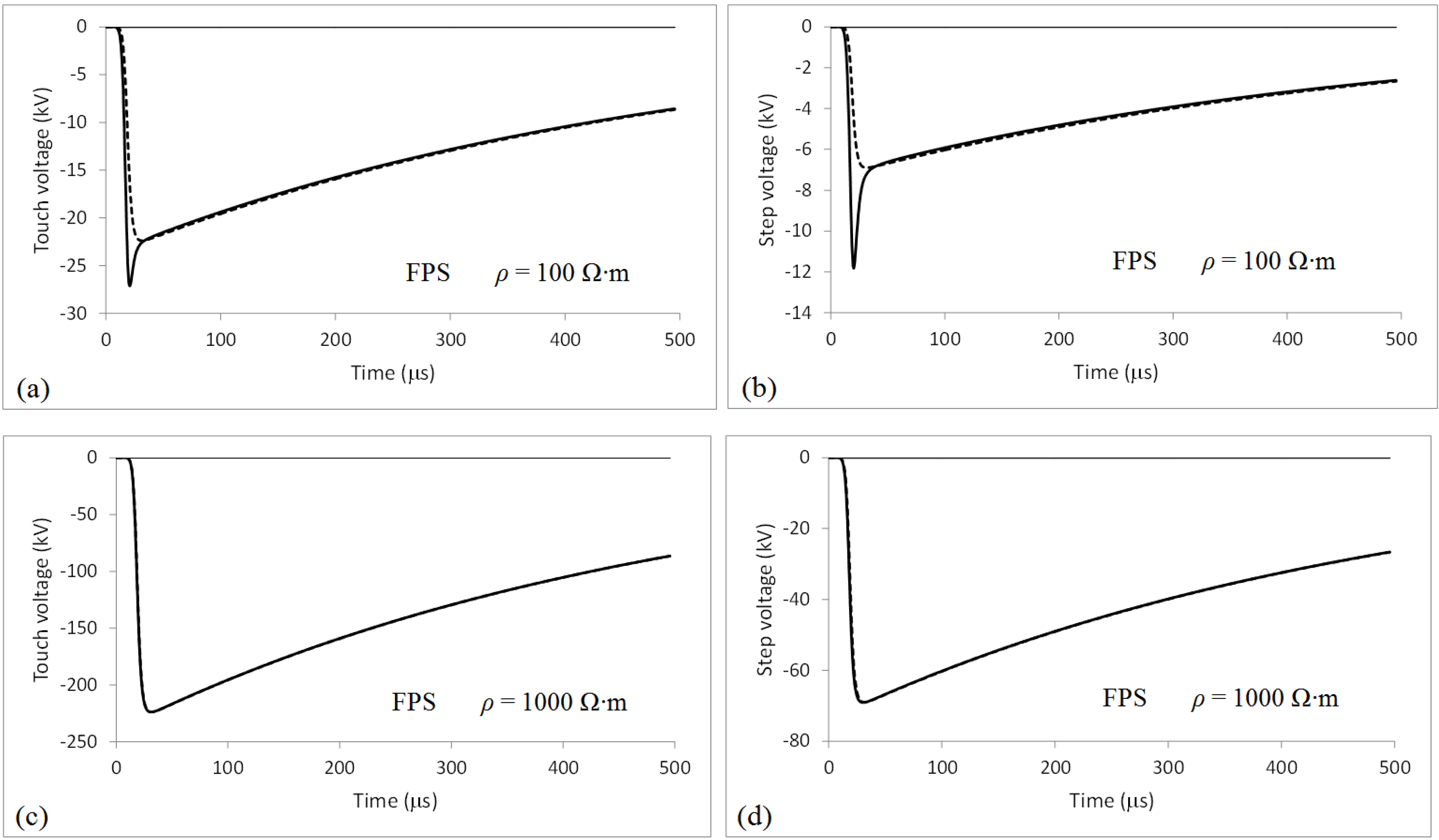
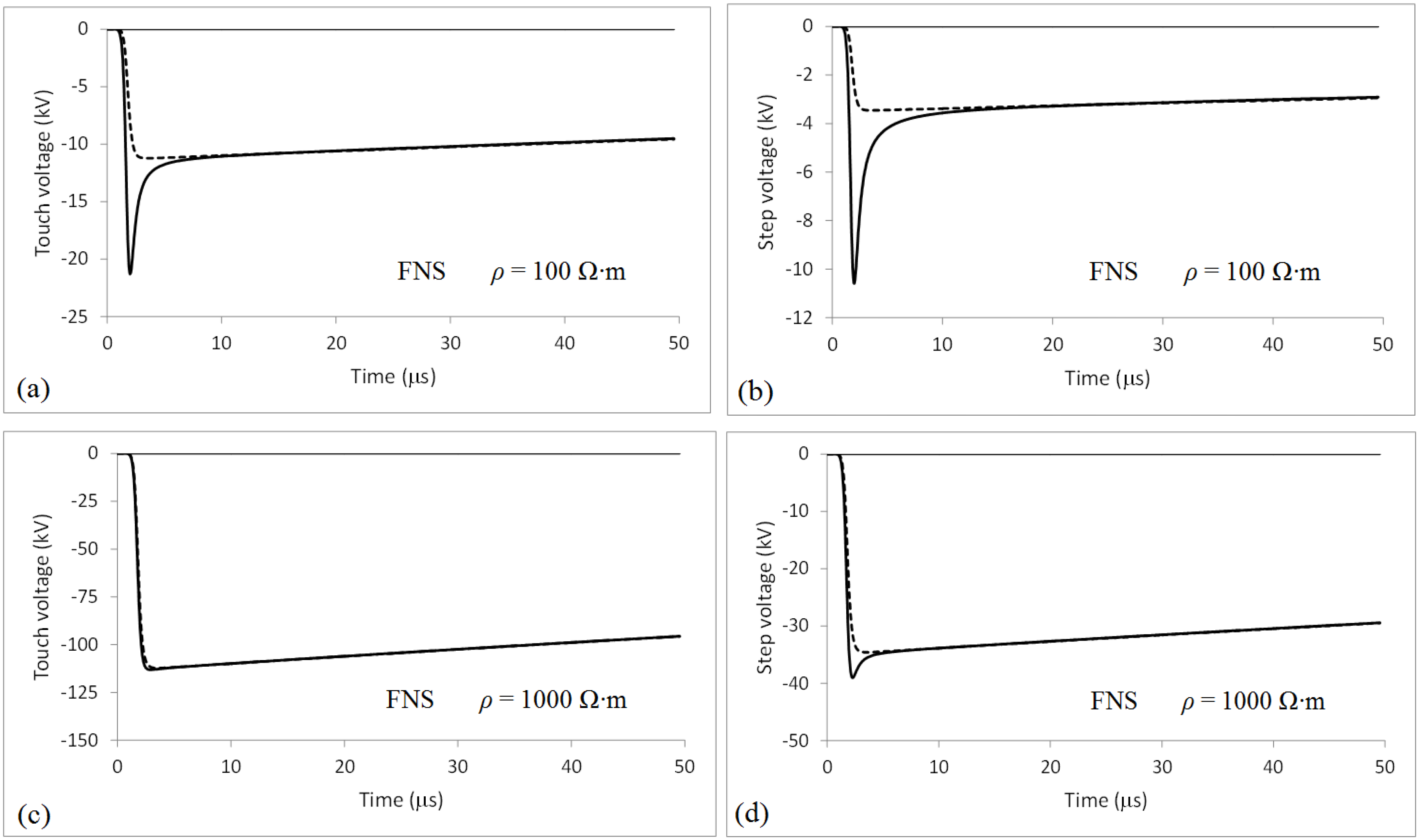
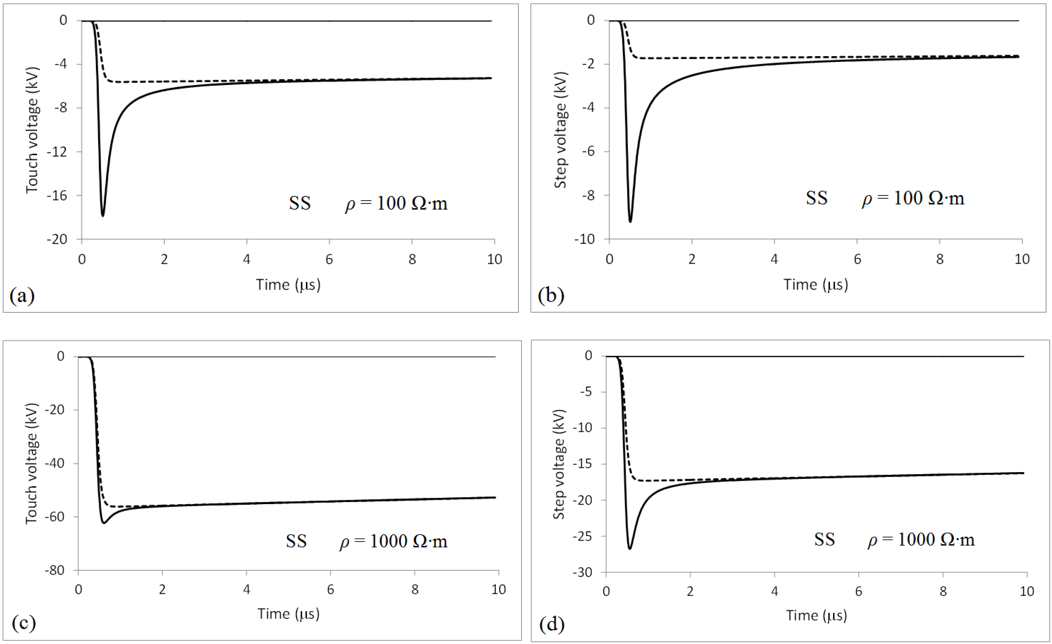
4. Touch and Step Voltages

This Section uses the author’s methodology, which was described and validated in the previous sections, to calculate the step and touch voltages in the vicinity of the structure. The structure basement is the same as considered in the previous section, i.e., a cylinder with 10 m radius and 8 m depth. The return stroke waveforms are those provided by the IEC standard [28] for the first positive stroke, first negative stroke, and subsequent stroke, with peak current values 200 kA, 100 kA, and 50 kA, respectively. These peak values correspond to lightning protection level I (LPL I) according to the standard, observing that the other levels differ from the first only by a scale factor. Therefore, the results can be replicated for LPL II and LPL III/IV by multiplying the waveforms from LPL I by the 0.75 and 0.5 scale factors. The waveshapes of these stroke currents are 10/350 μs, 1/200 μs, and 0.25/100 μs for first positive stroke, first negative stroke, and subsequent stroke, respectively.
Touch voltage is defined as the voltage between a person standing 1 m from the structure and touching it. In this paper, the voltage induced in the loop formed by the body of the person and the structure is neglected in front of the much higher voltage usually developed in lossy ground. However, it is worth mentioning that in some circumstances (e.g., subsequent stroke current and good-conducting ground) the voltage induced in the body loop may be relevant. Therefore, the touch voltage values presented in this paper correspond to the horizontal electric field calculated at 10.5 m from the structure axis, multiplied by 1 m. It can be demonstrated that the field at 10.5 m is very close to the average field from 10 to 11 m.
Step voltage is defined as the voltage between the two feet of a person due to a 1 m step. Similarly, the voltage induced in the loop formed by the legs of the person is neglected in front of the much higher voltage usually developed in lossy ground. However, it worth mentioning that in some circumstances (e.g., subsequent stroke current and good-conducting ground) the voltage induced in the body loop may be relevant. Therefore, the step voltage values presented in this paper correspond to the horizontal electric field calculated at 20 m from the structure axis, multiplied by 1 m. The distance value of 20 m was arbitrarily chosen in order to represent a nearby point that is likely to be assessed by the public. In order to evaluate the errors involved in calculating step and touch voltages based on the DC electric field, the values obtained with Equation (13) are also presented alongside those from the transient calculation.
Figure 6 shows the touch and step voltages for the first positive stroke, considering two ground resistivity values: 100 and 1000 Ω∙m. It can be seen in Figure 6 that for poor conducting ground (ρ ≥ 1000 Ω∙m), touch and step voltages can be accurately predicted for the first positive stroke by the DC method. However, for good conducting ground (ρ ≤ 100 Ω∙m), the transient method provides a significantly higher value. The difference between the voltages provided by the transient method and the DC method increases with increasing distance from the structure.
Figure 7 shows the touch and step voltages for the first negative stroke, considering two ground resistivity values: 100 and 1000 Ω∙m. It can be seen that for poor conducting ground (ρ ≥ 1000 Ω∙m), touch voltages can be accurately predicted and step voltages can be approximately predicted for the first negative stroke by the DC method. However, for good conducting ground (ρ ≤ 100 Ω∙m), the transient method provides much higher peak values than the DC approximation, for both touch and step voltages.
Figure 8 shows the touch and step voltages for the subsequent stroke, considering two ground resistivity values: 100 and 1000 Ω∙m. It can be seen that for poor conducting ground (ρ ≥ 1000 Ω∙m), touch voltages can be approximately predicted for the subsequent stroke by the DC method, but step voltages cannot. For good conducting ground (ρ ≤ 100 Ω∙m), the DC approximation largely underestimates the peak values for both the touch and step voltages. Table 3 summarizes the peak values of the touch and step voltages calculated from Equation (4).

5. Discussion

An approximate expression was proposed in Section 2.2 to represent the late-time horizontal electric field at the ground surface in the vicinity of a buried cylinder. Considering that its results agreed well with those from the FDTD calculation, it is interesting to further investigate this formulation. By integrating the horizontal electric field as per Equation (13) from the foundation border to infinity, and dividing the result by the current, the DC resistance of the cylindrical electrode can be obtained as:
R = ρ 2 π ( d r / 2 ) ln [ d + r / 2 r ]
It is worth mentioning that the condition dr / 2 in (19) leads to:
R = ρ 2 π r
which corresponds to the resistance of a hemisphere of radius r. Inserting the values d = 8 m and r = 10 m in Equation (19) provides R = 13.9 Ω for 1000 Ω∙m ground. This value is 87% of the resistance value of a hemisphere of radius r = 10 m (15.9 Ω).
The FDTD results [2] used as reference in Section 3 considered that the current propagation velocity was equal to the velocity of light in free space, both along the structure and the lightning channel. However, in real life the velocity of propagation along the lightning channel is lower than the velocity of light. As the close horizontal electric field at ground level is strongly determined by the current at the structure base, the return stroke velocity is unlikely to significantly affect the results. It is worth mentioning that this subject has been investigated for a point of interest relatively far from the structure [38,39,40].
In Section 2.1, it was considered that the sources of radiation are located only at the structure top and bottom, because at these points the charges are accelerated. This is true if the structure is considered as an uniform and lossless transmission line. However, even if the losses in the structure could be neglected, its impedance is not uniform. The continuous impedance variation changes the current waveform as it travels along the structure and produces a small radiation along the structure. In any case, as the results presented in Section 3 depicted, this effect can be neglected for most practical applications.
The IEC standard [1] recommends a 100 kV insulation level to protect against impulsive touch voltages. For the structure dimensions considered in this paper and ground resistivity equal to or lower than 1000 Ω∙m, the results of Section 3 show that this insulation level is sufficient for subsequent strokes, is slightly exceeded by first negative strokes, and is largely exceeded by first positive strokes (considering LPL I). However, as stated in the standard, the services connected to the structure (e.g, power cables, telecommunication cables, and water pipes) are likely to carry a significant part of the lightning current. The standard suggests that only half of the stroke current is likely to flow through the structure grounding system and foundation, with the remaining current being shared by the services. Considering this approximation and the conditions of Section 4, it turns out that the 100 kV insulation level proposed by the standard is likely to withstand the impulsive touch voltages due to a lightning flash.

6. Conclusions

The formula proposed by Barbosa and Paulino, complemented to take into account the effect of the structure foundation, was used to calculate the horizontal electric field at the ground surface in the vicinity of a structure hit by lightning. The input for the calculation is the current waveform at the structure base, and the results agreed well with those obtained by Baba and Rakov using FDTD [2]. The agreement between these results shows that the placement of the channel base at the structure top does not significantly influence the results.
The application of the method described in this paper shows that the use of DC approximation to calculate touch and step voltages may lead to significant errors, especially for fast-rising currents and relatively good-conducting soils. This means that DC approximation could be used for positive first stroke and poor conducting ground (ρ ≥ 1000 Ω∙m), but cannot be used for subsequent strokes and good-conducting ground (ρ ≤ 100 Ω∙m). Moreover, step voltages differ more from the DC approximation than the touch voltages.

Acknowledgments

This work was partially supported by CNPq (Brazilian National Council for Scientific and Technological Development).

Conflicts of Interest

The author declares no conflict of interest.

References

  1. IEC-62305–3. Protection against Lightning—Part 3: Physical Damage to Structures and Life Hazard; IEC: Alexandria, VA, USA, 2010. [Google Scholar]
  2. Baba, Y.; Rakov, V.A. Influence of strike object grounding on close lightning electric fields. J. Geophys. Res. 2008, 113, 1–18. [Google Scholar] [CrossRef]
  3. Sommerfeld, A. Uber die Ausbreitung der Wellen in der drahtlosen Telegraphie. Ann. d. Phys. 1909, 28, 4–8. [Google Scholar] [CrossRef]
  4. Sommerfeld, A. Partial Differential Equations in Physics—Lectures on Theoretical Physics VI—Chapter VI: Problems of Radio; Academic Press: New York, NY, USA, 1949. [Google Scholar]
  5. Zeddam, A.; Degauque, P. Current and voltage induced on a telecommunication cable by a lightning stroke. Electromagnetics 1987, 7, 541–564. [Google Scholar] [CrossRef]
  6. Delfino, F.; Procopio, R.; Rossi, M.; Rachidi, F.; Nucci, C.A. An algorithm for the exact evaluation of the underground lightning electromagnetic fields. IEEE Trans. Elect. Comp. 2007. [Google Scholar] [CrossRef]
  7. Delfino, F.; Procopio, R.; Rossi, M. Lightning return stroke current radiation in presence of a conducting ground: 1. Theory and numerical evaluation of the electromagnetic fields. J. Geophys. Res. 2008. [Google Scholar] [CrossRef]
  8. Delfino, F.; Procopio, R.; Rossi, M.; Rachidi, F.; Nucci, C.A. Lightning return stroke current radiation in presence of a conducting ground: 2. Validity assessment of simplified approaches. J. Geophys. Res. 2008. [Google Scholar] [CrossRef]
  9. Delfino, F.; Procopio, R.; Rossi, M.; Rachidi, F. Influence of frequency dependent soil electrical parameters on the evaluation of lightning electromagnetic fields in air and underground. J. Geophys. Res. 2009. [Google Scholar] [CrossRef]
  10. Delfino, F.; Procopio, R.; Rossi, M.; Shoory, A.; Rachidi, F. Lightning electromagnetic radiation over a stratified conducting ground−Part I: Formulation and numerical evaluation of the electromagnetic fields. J. Geophys. Res. 2011. [Google Scholar] [CrossRef]
  11. Shoory, A.; Rachidi, F.; Delfino, F.; Procopio, R.; Rossi, M. Lightning electromagnetic radiation over a stratified conducting ground−Part II: Validity of simplified approaches. J. Geophys. Res. 2011. [Google Scholar] [CrossRef]
  12. Cooray, V. Horizontal fields generated by return strokes. Radio Sci. 1992, 27, 529–537. [Google Scholar] [CrossRef]
  13. Rubinstein, M. An approximate formula for the calculation of the horizontal electric field from lightning at close, intermediate and long range. IEEE Trans. Elect. Comp. 1996, 38, 531–535. [Google Scholar] [CrossRef]
  14. Rachidi, F.; Rubinstein, M.; Zweiacker, P.; Ianoz, M.; Braendli, P.; Kaelin, A. Indirect lightning effects on short overhead lines. Int. Symp. Electromagn. Comp. 1998, 98, 345–349. [Google Scholar]
  15. Borghetti, A.; Nucci, C.A.; Paolone, M. An improved procedure for the assessment of overhead line indirect lightning performance and its comparison with the IEEE STD. 1410 Method. IEEE Trans. Power Deliv. 2007, 22, 684–692. [Google Scholar] [CrossRef]
  16. Cooray, V. Horizontal electric field above and underground produced by lightning flashes. IEEE Trans. Elect. Comp. 2010, 52, 936–943. [Google Scholar] [CrossRef]
  17. Barbosa, C.F.; Paulino, J.O.P. An approximate time domain formula for the calculation of the horizontal electric field from lightning. IEEE Trans. Elect. Comp. 2007, 49, 593–601. [Google Scholar] [CrossRef]
  18. Paulino, J.O.S.; Barbosa, C.F.; Lopes, I.J.S.; Boaventura, W.C. Assessment and analysis of indirect lightning performance of overhead lines. Electri. Power Sys. Res. 2015, 118, 55–61. [Google Scholar] [CrossRef]
  19. Paulino, J.O.S.; Barbosa, C.F.; Lopes, I.J.S.; Boaventura, W.C.; Miranda, G.C. Indirect lightning performance of aerial distribution lines considering the induced-voltage waveform. IEEE Trans. Elect. Comp. 2015, 57, 1123–1131. [Google Scholar] [CrossRef]
  20. Caligaris, C.; Delfino, F.; Procopio, R. Cooray-Rubinstein formula for the evaluation of lightning radial electric fields: Derivation and implementation in the time domain. IEEE Trans. Elect. Comp. 2008, 50, 194–197. [Google Scholar] [CrossRef]
  21. Delfino, F.; Girdinio, P.; Procopio, R.; Rossi, M.; Rachidi, F. Time-domain implementation of Cooray–Rubinstein Formula via convolution integral and rational approximation. IEEE Trans. Elect. Comp. 2011, 53, 755–763. [Google Scholar] [CrossRef]
  22. Andreotti, A.; Rachidi, F.; Verolino, L. A new formulation of the Cooray–Rubinstein expression in time domain. IEEE Trans. Elect. Comp. 2015, 57, 391–396. [Google Scholar] [CrossRef]
  23. Barbosa, C.F.; Paulino, J.O.S. A time-domain formula for the horizontal electric field at the earth surface in the vicinity of lightning. IEEE Trans. Elect. Comp. 2010, 52, 640–645. [Google Scholar] [CrossRef]
  24. Cooray, V. Horizontal electric field at ground level in the vicinity of lightning return stroke channels evaluated using Sommerfeld’s integrals. In Processing of the 29th International Conference on Lightning Protection, Uppsala, Sweden, 23–26 June 2008.
  25. Paulino, J.O.S.; Barbosa, C.F.; Lopes, I.J.S.; Miranda, G.C. Time-domain analysis of rocket-triggered lightning-induced surges on an overhead line. IEEE Trans. Elect. Comp. 2009, 51, 725–732. [Google Scholar] [CrossRef]
  26. Paulino, J.O.S.; Barbosa, C.F.; Boaventura, W.C. Effect of the surface impedance on the induced voltages in overhead lines from nearby lightning. IEEE Trans. Elect. Comp. 2011, 53, 749–754. [Google Scholar] [CrossRef]
  27. Paulino, J.O.S.; Barbosa, C.F.; Boaventura, W.C. Lightning-induced current in a cable buried in the first layer of a two-layer ground. IEEE Trans. Elect. Comp. 2014, 56, 956–963. [Google Scholar] [CrossRef]
  28. IEC-62305–1. Protection against Lightning−Part 1: General Principles; IEC: Alexandria, VA, USA, 2010. [Google Scholar]
  29. Uman, M.A.; McLain, D.K. Magnetic field of lightning return stroke. J. Geophys. Res. 1969, 74, 6899–6910. [Google Scholar] [CrossRef]
  30. Rusck, S. Induced lightning overvoltages on power transmission lines with special reference to the overvoltage protection of low voltage networks. Trans. Royal Inst. Tech. 1958, 120, 55–69. [Google Scholar]
  31. Cooray, V.; Cooray, G. The deep physics hidden within the field expressions of the radiation fields of lightning return strokes. Atmosphere 2016. [Google Scholar] [CrossRef]
  32. Hallén, E. Lösung zweir potentialprobleme der elektrostatic. Arkif. Matematik. Astronomi. Och Fysik. 1929, 21, 35–39. [Google Scholar]
  33. Dwight, H.B. Calculation of resistances to ground. Trans. AIEE 1936, 55, 1319–1328. [Google Scholar]
  34. Barbosa, C.F. On the vertical ground rod resistance with special reference to thick rods. In Proceedings of International Conference on Grounding and Earthing, Porto de Galinhas, Brazil, 10–16 June 2016.
  35. Heidler, F.; Manhardt, M.; Stimper, K. Upward positive lightning measured at the Peissenberg Tower, Germany. Int. Symp. Light. Prot., SIPDA 2013. [Google Scholar] [CrossRef]
  36. Heidler, F. Analitsche blitzstromfunktion zur LEMP-berechnung. In Proceedings of 18th International Conference Lightning Protection, Munich, Germany, 2–9 August 1985.
  37. Greenwood, A. Electrical Transients in Power Systems—Section 2.6: Duhamel’s Integral - Response of A Circuit to An Arbitrary Stimulus; John Wiley Sons: Hoboken, NJ, USA, 1971. [Google Scholar]
  38. Baba, Y.; Rakov, V.A. Voltages induced on an overhead wire by lightning strikes to a nearby tall grounded object. IEEE Trans. Elect. Compat. 2006, 48, 212–224. [Google Scholar] [CrossRef]
  39. Rachidi, F.; Janischewskyj, W.; Hussein, A.M.; Nucci, C.A.; Guerrieri, S.; Kordi, B.; Chang, J.S. Current and electromagnetic field associated with lightning return strokes to tall towers. IEEE Trans. Elect. Comp. 2001, 43, 3–9. [Google Scholar] [CrossRef]
  40. Rakov, V.A. Transient response of a tall object to lightning. IEEE Trans. Elect. Comp. 2001, 43, 654–661. [Google Scholar] [CrossRef]
Figure 1. (a) Return stroke at the ground level; (b) Return stroke at the top of the structure.
Atmosphere 07 00115 g001
Figure 2. Cylindrical electrode and its approximate equipotential surfaces.
Atmosphere 07 00115 g002
Figure 3. Conical structure with a cylindrical foundation considered for the calculation.
Atmosphere 07 00115 g003
Figure 4. Current values at the structure base. Solid line: analytical Equation (15); Dots: extracted from [2]. Ground resistivity values (a) 100 Ω∙m; (b) 1000 Ω∙m.
Atmosphere 07 00115 g004
Figure 5. Horizontal electric field at the ground surface for different values of ground resistivity (ρ) and distance from the structure axis (x). Solid line: analytical Equation (4); Dots: extracted from [2]. (a) ρ = 100 Ω∙m; x = 15 m; (b) ρ = 100 Ω∙m; x = 30 m; (c) ρ = 100 Ω∙m; x = 60 m; (d) ρ = 1000 Ω∙m; x = 15 m; (e) ρ = 1000 Ω∙m; x = 30 m; (f) ρ = 1000 Ω∙m; x = 60 m.
Atmosphere 07 00115 g005aAtmosphere 07 00115 g005b
Figure 6. Touch voltage (TV) and step voltage (SV) for first positive stroke (FPS). Solid line: transient response calculated from Equation (4); Dashed line: DC response calculated from Equation (13). (a) TV and ρ = 100 Ω∙m; (b) SV and ρ = 100 Ω∙m; (c) TV and ρ = 1000 Ω∙m; (d) SV and ρ = 1000 Ω∙m.
Atmosphere 07 00115 g006
Figure 7. Touch voltage (TV) and step voltage (SV) for first negative stroke (FNS). Solid line: transient response calculated from Equation (4); Dashed line: DC response calculated from Equation (13). (a) TV and ρ = 100 Ω∙m; (b) SV and ρ = 100 Ω∙m; (c) TV and ρ = 1000 Ω∙m; (d) SV and ρ = 1000 Ω∙m.
Atmosphere 07 00115 g007
Figure 8. Touch voltage (TV) and step voltage (SV) for subsequent stroke (SS). Solid line: transient response calculated from Equation (4); Dashed line: DC response calculated from Equation (13). (a) TV and ρ = 100 Ω∙m; (b) SV and ρ = 100 Ω∙m; (c) TV and ρ = 1000 Ω∙m; (d) SV and ρ = 1000 Ω∙m.
Atmosphere 07 00115 g008
Table 1. Heidler function parameters for 100 Ω∙m ground resistivity.
ComponentDelay (μs)I (kA)τ1 (μs)τ2 (μs)n
10.5311.40.071.352
20.534.602.3122
31.601.900.080.332
42.670.380.080.332
Table 2. Heidler function parameters for 100 Ω∙m ground resistivity.
ComponentDelay (μs)I (kA)τ1 (μs)τ2 (μs)n
10.5310.30.071.502
20.534.302.1252
31.602.200.080.402
42.670.240.080.402
Table 3. Peak values (in kV) of the touch and step voltages calculated from Equation (4).
VoltageResistivity (Ω∙m)First Positive StrokeFirst Negative StrokeSubsequent Stroke
Touch100272118
100022411362
Step10012119
1000693927

