Article

Mie LIDAR Observations of Tropospheric Aerosol over Wuhan

1
State Key Laboratory of Information Engineering in Surveying, Mapping and Remote Sensing (LIESMARS), Wuhan University, Wuhan 430079, China
2
International Research Center of Satellite Remote Sensing and Atmospheric Monitoring, Wuhan University, Wuhan 430079, China
*
Author to whom correspondence should be addressed.
Atmosphere 2015, 6(8), 1129-1140; https://doi.org/10.3390/atmos6081129
Submission received: 13 May 2015 / Accepted: 3 August 2015 / Published: 7 August 2015

Abstract

:
Wuhan is a rapidly developing large city in central China. To analyze the aerosol characteristics over Wuhan, the optical properties of the nocturnal aerosol layers in the lower troposphere were observed using a ground-based LIDAR(Light Detection And Ranging) located in the Laboratory of Information Engineering in Surveying, Mapping and Remote Sensing (LIESMARS) from Wuhan University, China (114°21′E, 30°32′N) in January 2013–January 2015. The vertical distribution and temporal variation of tropospheric aerosols over Wuhan were summarized. The atmospheric boundary layer height (ABLH) was mainly at an altitude of 1.5–2 km (~33.1% probability), with an annual average of 1.66 km. The ABLH was higher in spring–summer (~2 km) and lower in autumn–winter (~1.2 km). The aerosol optical depth (AOD) was higher in spring–autumn than in summer–winter. The highest AOD was about 0.79 in October and the lowest was about 0.08 in January. The annual average was about 0.3. To study the relationship between the AOD and the particulate matter ≤2.5 µm in the aerodynamic diameter (PM2.5) in the lower troposphere, a typical haze event from 9–14 October 2014 was investigated. The results showed a correlation coefficient of 0.5165 between these two variables.

1. Introduction

Aerosols play a major role in the assessment of climate, Earth’s radiation, the formation of clouds and precipitation, and environmental problems [1]. The Intergovernmental Panel on Climate Change (IPCC) has reported that large uncertainties on climate change are attributed to both the direct and indirect effect of aerosols [2]. They have also been considered to be the greatest contributors to the total uncertainty in radiative forcing because of their direct and indirect effects. Thus, investigation of the spatiotemporal distribution of tropospheric aerosols is very important for understanding aerosol radiative forcing [3].
The current primary means of detecting aerosols is the AERONET monitoring network [4], which can provide aerosol column information but is unable to obtain its accurate vertical distribution. However, LIDAR (Light Detection And Ranging) detection systems have been developed and widely used for this purpose. The European Aerosol Research LIDAR Network (EARLINET) was the first aerosol LIDAR network mainly aimedat providing a comprehensive, quantitative, and statistically significant database for the aerosol distribution on a continental scale [5]. Matthias et al. studied the vertical distribution of aerosols over Europe [6]. In the US, the Micro Pulse LIDAR Network (MPLNET) was initiated by NASA (National Aeronautics and Space Administration), covering more area and supporting a wide range of atmospheric aerosols. Welton et al. [7] monitored global changes in clouds and aerosols. In Japan, the National Institute for Environmental Studies (NIES) also has a LIDAR Monitoring Network, which is called AD-NET (Sugimoto and Huang, 2014) [24]. Hayashida et al. [8] observed the volcanic disturbances in the stratospheric aerosol layer over Tsukuba, Japan. Some Chinese institutions such as the Anhui Institute of Optics and Fine Mechanics [9], Xi'an University of Technology [10], the Institute of Atmospheric Physics [11], and Lanzhou University [12] are also studying LIDAR systems to detect aerosols. Examples of studies are given by Yan et al. [13], who observed the boundary layer structure and aerosol properties over Xi'an, Jinhuan et al. [14], who analyzed the variation characteristics of the atmospheric aerosol optical depths and visibility in North China, and Huang et al. [15], who detected the dust aerosol vertical structure. For heavily industrialized cities such as Wuhan, Zhang et al. [16] analyzed the aerosol optical properties for a haze episode and Gong et al. [17,18] studied the aerosol optical properties and determined their size distribution. Nevertheless, research on the atmospheric boundary layer height (ABLH) and aerosol annual optical properties is relatively scarce. To fill this gap, the annual changes in aerosol optical characteristics and ABLH were studied for Wuhan.
Our study of the vertical structure and optical properties of the aerosol layer was performed using ground-based LIDAR. The LIDAR uses aerosols as tracers, which, through scattering, contribute to the backscatter intensity of the range-resolved measurement. Accordingly, the height and optical properties of the aerosol layer were determined from the LIDAR signal. We used two years of LIDAR data (January 2013–January 2015) to investigate the vertical structure and optical properties of the aerosol layer in Wuhan. The distribution of the ABLH was analyzed and the seasonal and monthly aerosol variation was studied. Finally, a typical haze event from 9–14 October 2014 was used to analyze the correlation between the concentration of air particles below 2.5 µm diameter (PM2.5) and the aerosol optical depth (AOD).

2. Study Site and Instrumentation Used

2.1. Study Site Location

The LIDAR system was located at Wuhan University (114°21′E, 30°32′N), Guangbutun, in the business center of Wuhan, about 39 m away from the ground and surrounded by buildings [18]. Wuhan City is one of China's largest industrial and commercial cities, with serious impacts on the air quality from industrial emissions. Its population reached 10.02 million in 2011, with 5.7 million in the center where the atmospheric pollution is largest. This region has a subtropical monsoon climate, with abundant rainfall and high temperatures in the summer and abundant cloud cover, relatively high humidity, and low temperatures in winter. Because of its sustained extremely high temperatures in the summer, Wuhan is known as one of China’s four furnaces.

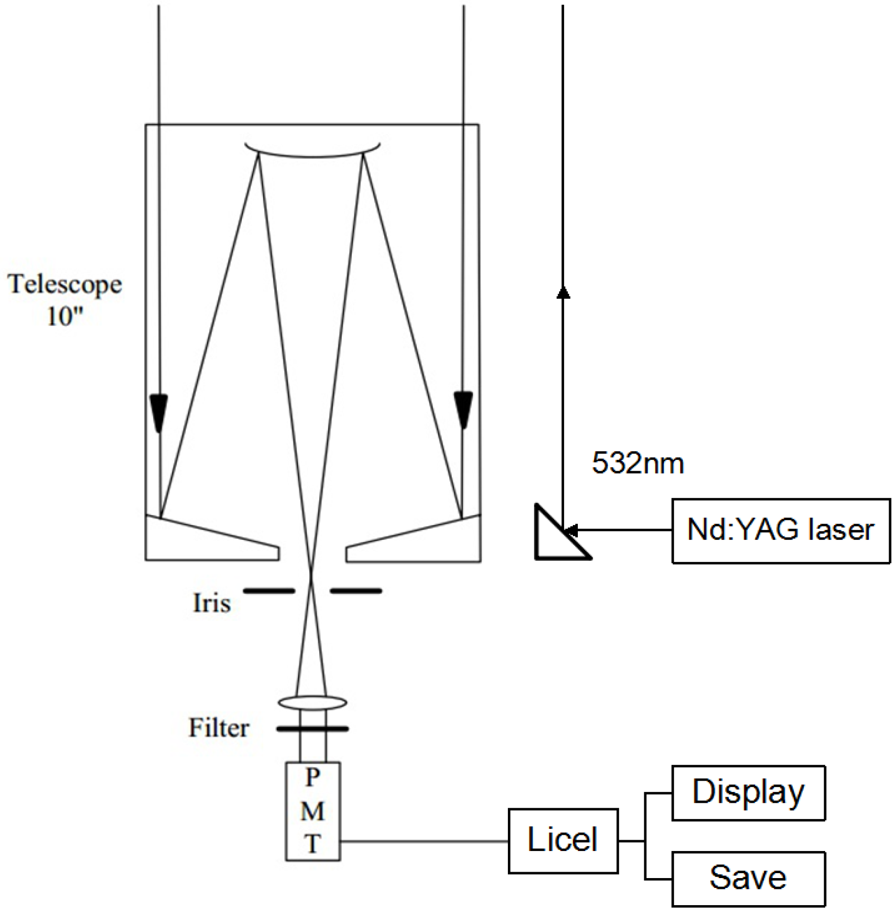
2.2. LIDAR System Description

The light detection and ranging system included a laser emitting, an optical receiving, and a signal acquisition system. The laser emitting system consisted of three parts: a Nd: YAG (Neodymium-doped Yttrium Aluminium Garnet)laser, a laser beam expander, and a mirror (Figure 1). The emission wavelength of the Nd: YAG pulsed laser was 532 nm, with a laser pulse width, energy, and repetition frequency of 10 ns, 140 mJ, and 20 Hz, respectively. The laser beam was Gaussian. To further compress the divergence angle of the laser beam, a beam expander was used. The optical receiver system consisted of three parts: a telescope, a collimating lens, and narrowband interference filters. The return LIDAR signal backscattered by the atmosphere was collected by a 10-inch (254 mm) diameter Schmidt-Cassegrain telescope. A narrowband filter was used to suppress the sky background components.
Figure 1. LIDAR image.
Atmosphere 06 01129 g001
The collected backscattered signals were detected by a photomultiplier tube (PMT) with a high-speed preamplifier in an analog detection mode and recorded by a 16-bit data acquisition (ADQ) card at a 40 MHz sampling rate. The backscattered signals measured by the ADQ were stored in a personal computer, with vertical and temporal resolutions of 3.75 m and 60 s, respectively. More details can be seen in Table 1.
Table 1. Mie LIDAR specifications.
Transmitter
Wavelength (nm)532, Nd: YAG
Pulse width (ns)10
Pulse repetition frequency (Hz)20
Maximum pulse energy (mJ)140
Laser beam divergence (mrad)0.5
Receiver
Optical designSchmidt-Cassegrain
Diameter of telescope (mm)254
Focal length (mm)2500
Filter bandwidth (nm)3
Field of view (mrad)1
Spatial resolution (m)3.75

3. Data Retrieval

The data processing consisted of two steps. First, the ideal profile fitting method to calculate the distribution of the boundary layer profile with the best stability for a good mixed situation to effectively obtain the ABLH by fitting the backscatter coefficient curve, was introduced [19]. Then, we obtained the distribution of the AOD and the extinction coefficient using the Fernald method [20,21,22,23], which regards the atmosphere as two components, for a more accurate calculation.

3.1. Ideal Profile Fitting Method

The ideal profile fitting method obtained the boundary layer parameters by fitting an atmosphere backscattering coefficient [19]. The atmospheric boundary layer becomes a mixed layer, characterized by approximate height invariant values for winds and scalar quantities under convective conditions. The mixed layer is capped by an entrainment zone, which provides a transition to the (often stable) lower troposphere. The mixed layer depth is of primary importance because it determines the volume of atmosphere through which surface-emitted pollutants can be diluted, and it is also a length scale governing the behavior of the largest scales of boundary layer turbulence [25]. Thus, we regard the mixed layer height as the ABLH top. The ideal profile was expressed by an error function:
X ( r ) = X m + X u 2 X m X u 2 e r f ( r r m s )
Where rm is the average depth of the boundary layer, Xm is the average of X(r), Xu is the averaged X(r) above the boundary layer, and s is related to the thickness of the entrainment layer. The above parameters were determined by least squares fitting the measured signal to the ideal profile. Finally, the ABLH was calculated.

3.2. Fernald Method

According to the Fernald method, the received laser pulse power P(r) from distance r can be described as a function of the volume extinction coefficient α(r) and the backscatter coefficient β(r) [21].
P ( r ) = C P 0 r 2 [ β m ( r ) + β a ( r ) ] exp [ 2 0 r [ α m ( r ) + α a ( r ) ] d r ] + P n b
Where C is a calibration constant including the losses in the transmitting and receiving optics and the effective receiver aperture, P0is an output monitor pulse whose amplitude is proportional to the transmitted energy, βm(r) and βα(r) are the backscattering coefficients of the aerosols and molecules at slant range r, respectively, αm(r) and αα(r) are the extinction cross-sections of the aerosols and molecules at range r, respectively, and Pnb is the background noise. The molecular atmosphere scattering properties, βm(r) and αm(r), were determined from the approximated appropriate standard atmospheres or the best available meteorological data, while the aerosol scattering properties, including βα(r) and αα(r), had to be determined. According to the research [26], they obtained the vertical distribution of the LIDAR ratio by the Raman scattering principle on September 12 2009 at Wuhan. They found that the LIDAR ratio fluctuated around 50 sr in the range of 3 km. Considering that larger-sized aerosols are dropping and the atmosphere becomes clearer as the night is falling, they took the average of the LIDAR ratio (50 sr).The corresponding ratio for the aerosol scatterers was constant for the Wuhan area (Sα = αα(r) / βα(r) = 50). The solution to Equation (2) for the aerosol backscattering coefficient then became:
β a ( r ) = P ( r ) r 2 exp [ 2 ( S a S m ) 0 r β m ( r ) d r ] C P 0 2 S a 0 r P ( r ) r 2 exp [ 2 ( S a S m ) 0 r β m ( r ' ) d r ' ] d r β m ( r )
The atmospheric extinction coefficient is an important parameter to study the properties of the boundary layer, while the quality of the atmosphere can be characterized by the AOD [22]. The AOD is the integral of the extinction coefficient (α(r)) along the optical path between R1and R2:
A O D = R 1 R 2 α ( r ) d r
In addition, there is an inherent problem with the Mie LIDAR, which is its overlap function. The overlap function of the Mie LIDAR has been calculated by a simple overlap factor calculation method based on laser intensity distribution [27].The relative error of the overlap factor correction is more than 20% when the range is below 200 m. Thus, we have removed the LIDAR signals from 0 to 200 m. Additionally, we used the least squares linear fitting to fit the range-corrected signal in the far range. Then we extrapolated the fitting function to get the range-corrected signals from 0 to 200 m. Finally, the range corrected signal was used to get the AOD inversion.

4. Results and Discussion

We interpreted the ABLH and aerosol characteristics from January 2013–January 2015 based on 151 observations between 7 p.m. and 7 a.m. the next day. According to the date, the spatiotemporal distribution of the tropospheric aerosols was analyzed.

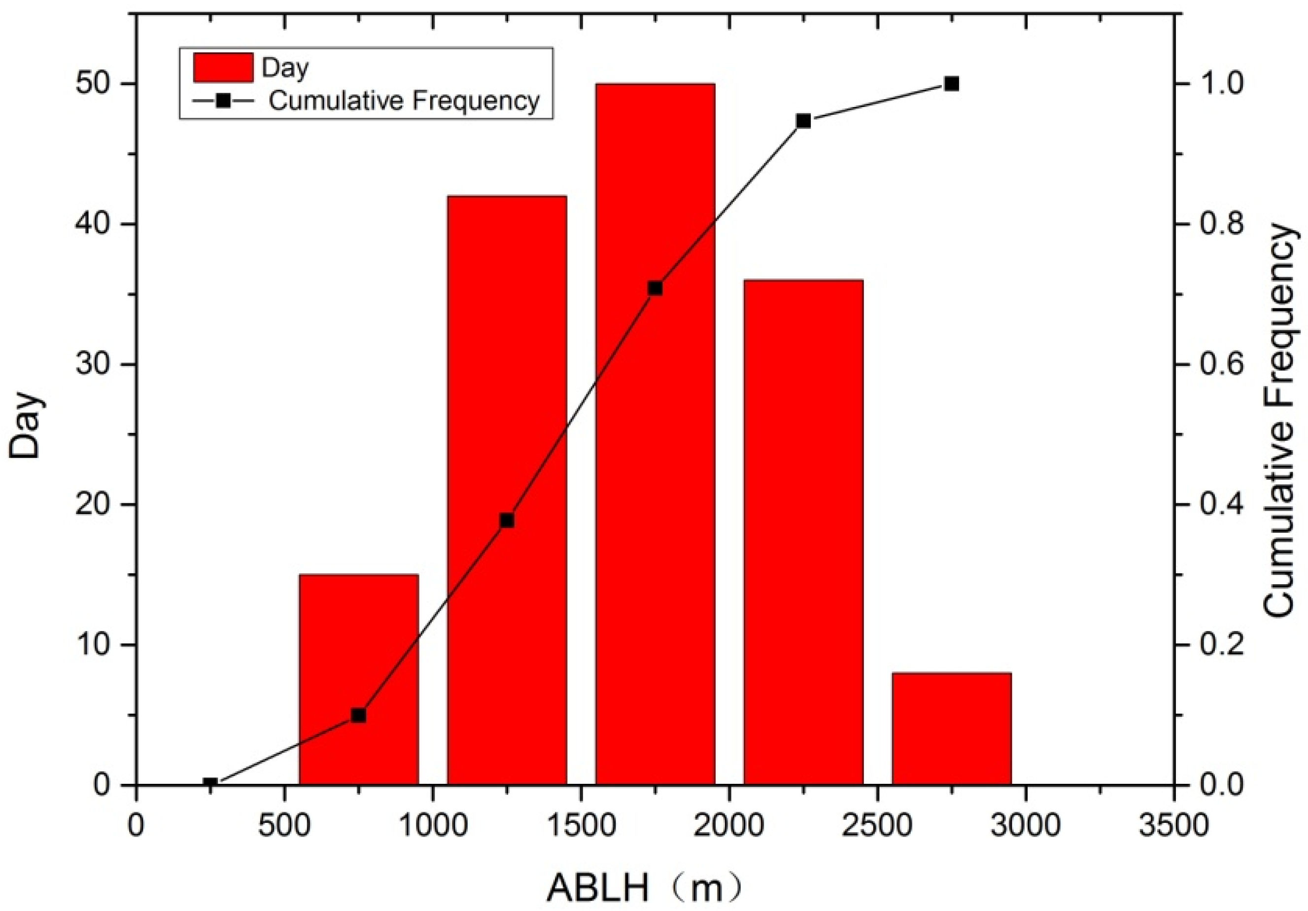
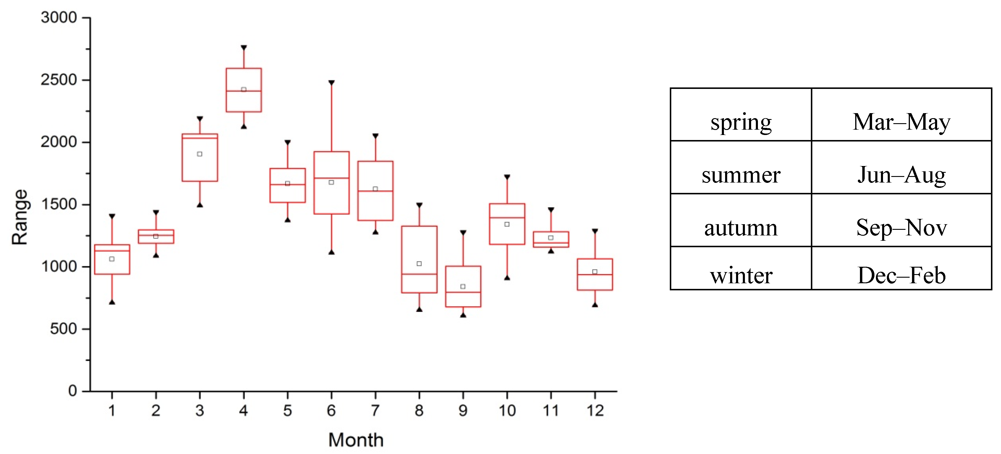
4.1. ABLH Characteristics

The statistics data represents the average height of the entire night atmospheric boundary layer. The frequency distribution histogram of the ABLH in Wuhan for 2013 and 2014 (Figure 2) shows an approximately normal distribution, with an ABLH of about 2 km in spring–summer and about 1.2 km in autumn–winter. A large fraction of the annual ABLH (33.1%) ranged 1.5–2 km, with an average of 1.66 km. In addition, it was mostly (70.8%) below 2 km.
Figure 2. Cumulative probability distribution and probability distribution of the atmospheric boundary layer height (ABLH). The black line represents the cumulative frequency and the red histogram shows the number of occurrences in days.
Atmosphere 06 01129 g002
Figure 3. Monthly statistics of the atmospheric boundary layer height (ABLH). The boxes represent the mean of the maximum and minimum for each month, the triangles represent the monthly maximum and minimum, and the short horizontal lines represent the monthly average.
Atmosphere 06 01129 g003
Figure 3 shows the monthly and seasonal variation of the ABLH. The rainy season of Wuhan is in the summer. Half of month is raining in May, June, and July. Thus, the result is probably low in May, June, and July. The maximum value was about 2.76 km in April, the minimum was about 0.67 km in September, and the annual average was about 1.66 km. Spring and summer had higher values, with the highest in spring, compared to autumn and winter, with the lowest value in autumn. In Wuhan, in spring–summer and March–August, because of the strong solar radiation and high surface temperatures, the atmospheric convective motion is frequent and intense, enhancing the diffusion of aerosols.

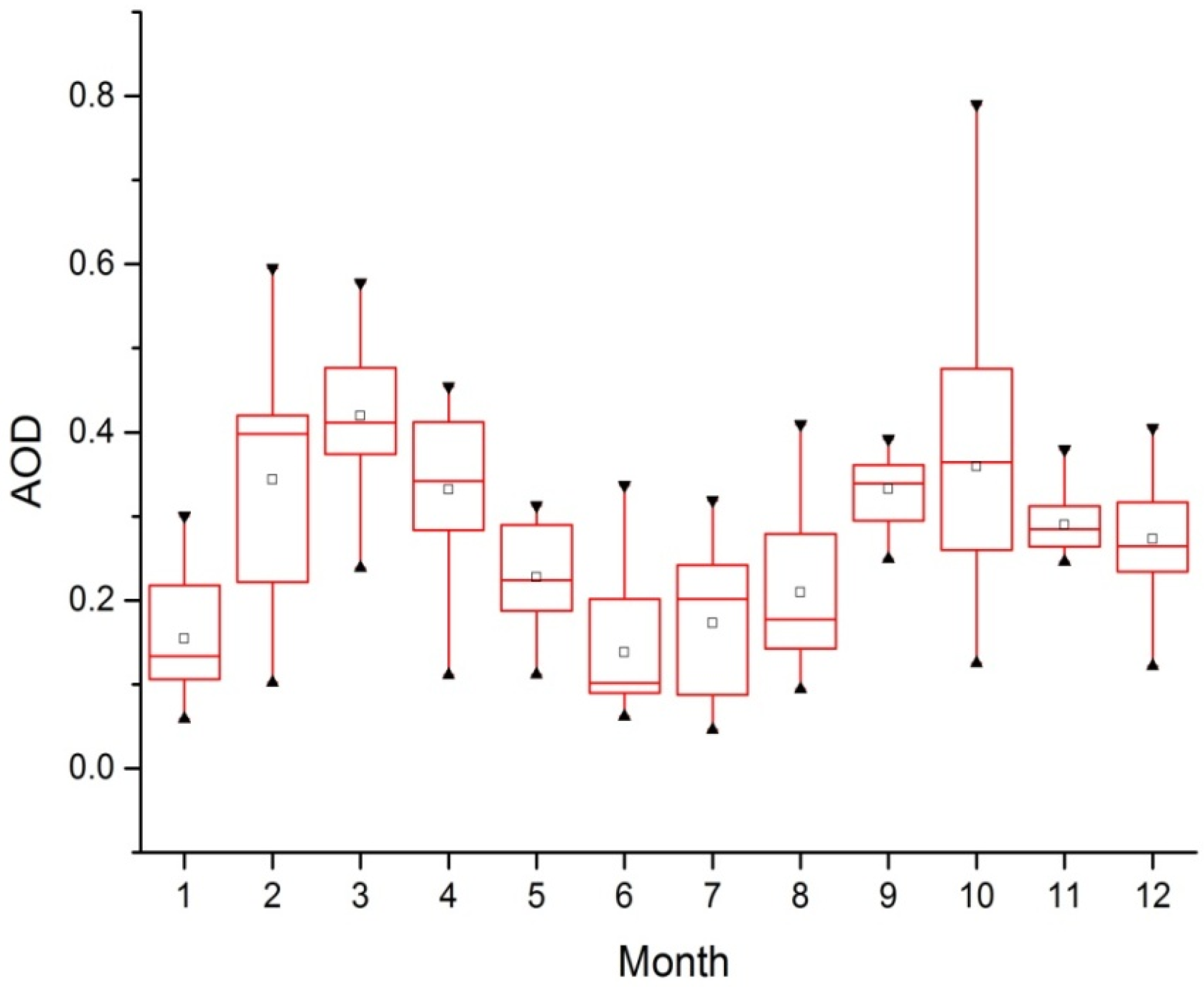
4.2. AOD Characteristics

Figure 4 depicts the variations of the monthly AOD at 532 nm in January–December. The highest AOD (~0.79) appeared in October, while the smallest (~0.08) appeared in January. The annual mean was about 0.3, with higher values in spring and autumn and lower values in summer and winter. The higher AOD in spring was probably caused by dust particles in the free troposphere transported from the north, while the summer values seemed to result from hygroscopic aerosols and abundant moisture in the mixing layer and intense turbulence near the ground.
Figure 4. Monthly statistics of the aerosol optical depth (AOD) at 532 nm. The boxes represent the mean of the maximum and minimum for each month, the triangles represent the monthly maximum and minimum, and the short horizontal lines represent the monthly average.
Atmosphere 06 01129 g004

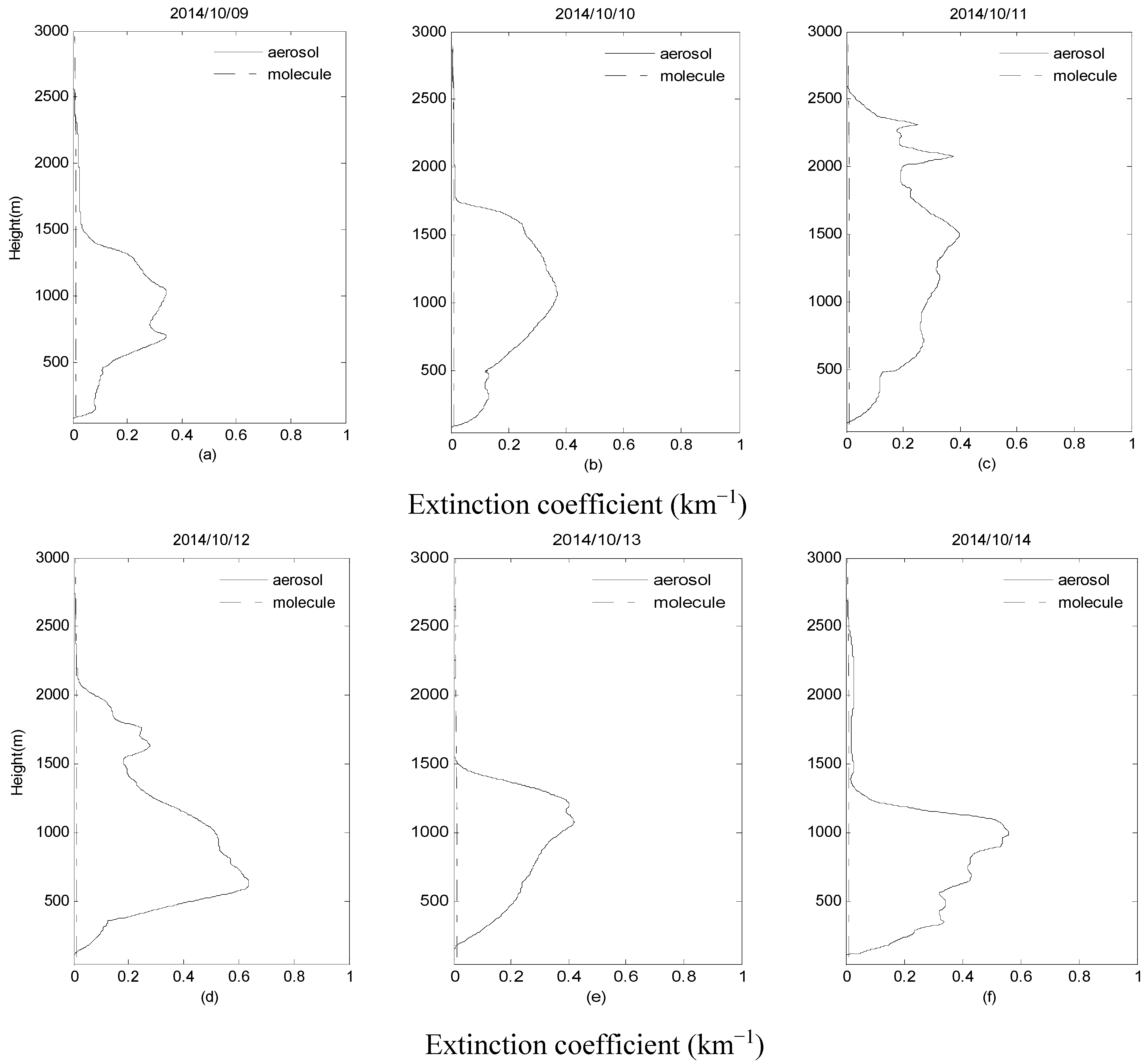
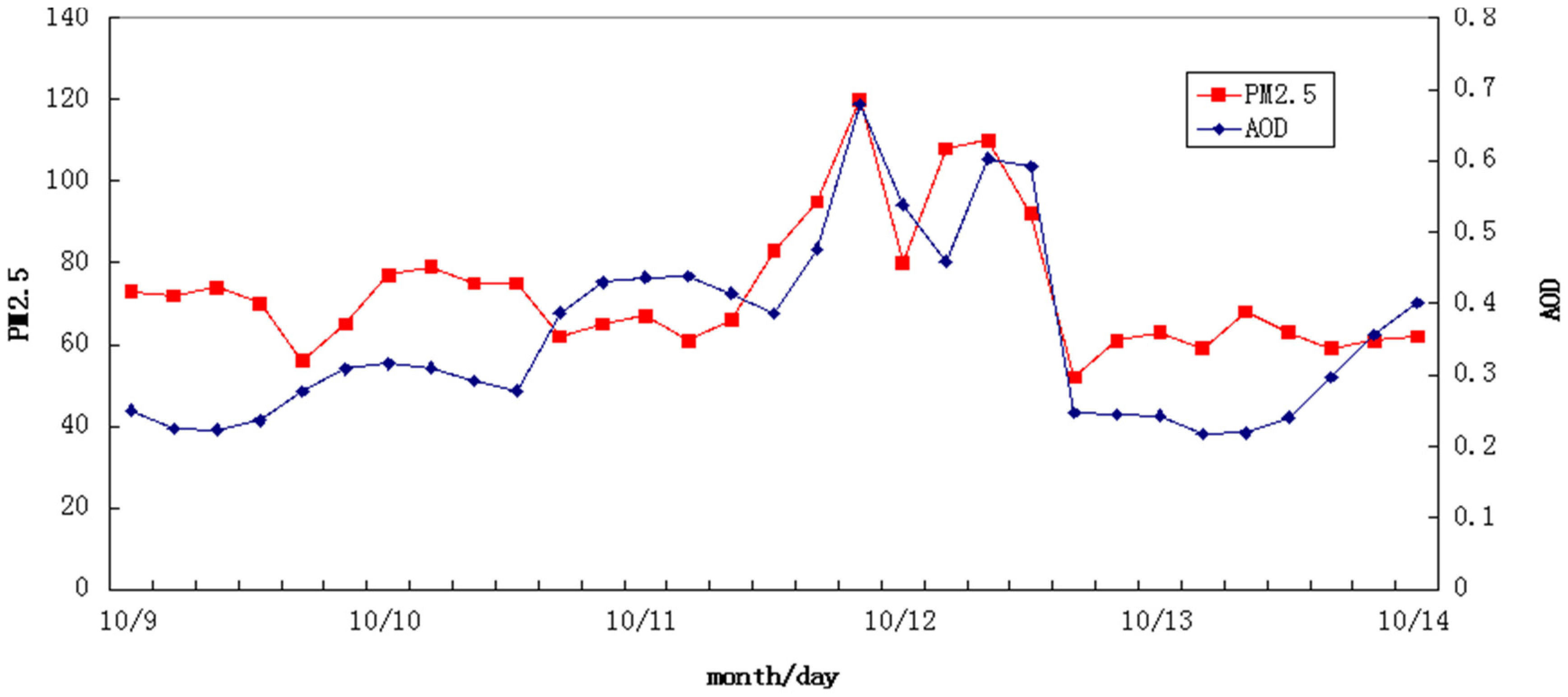
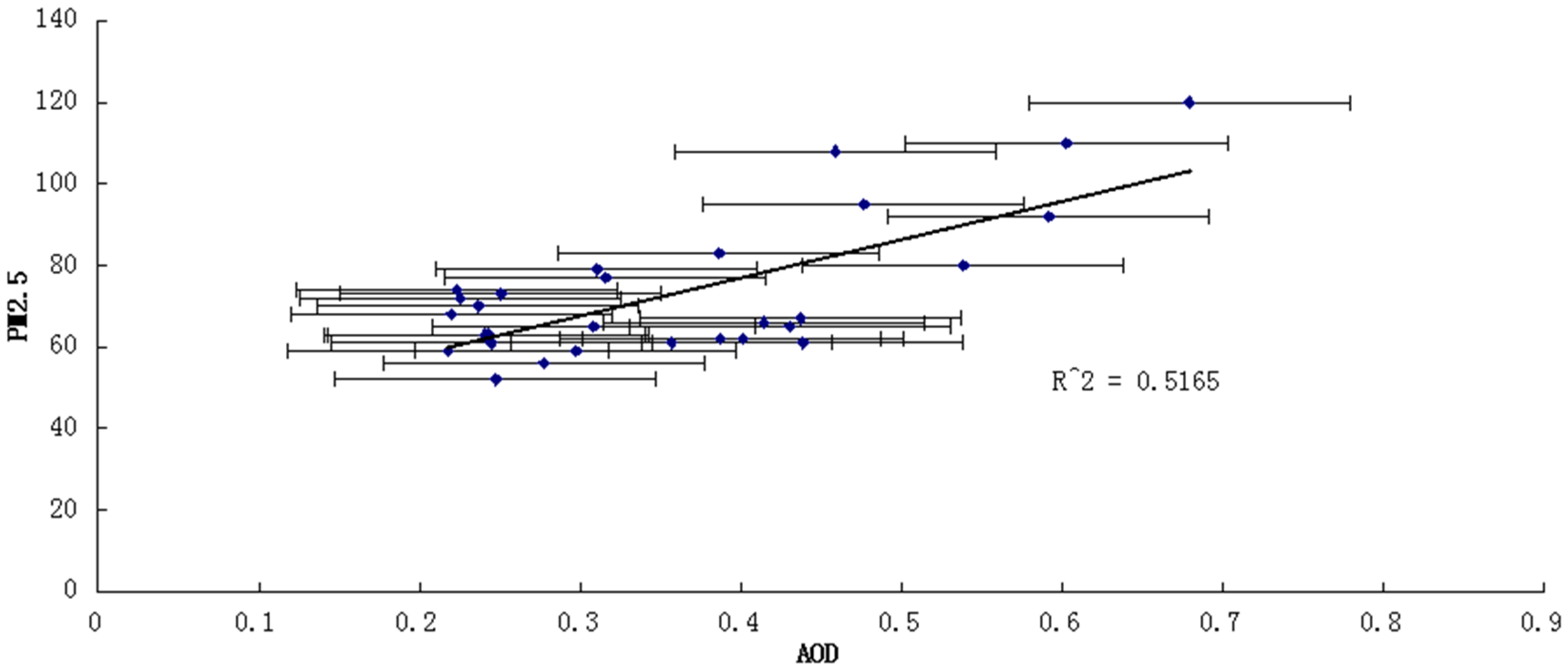
4.3. Haze Event Analysis

A typical haze event on 9–14 October 2014 was analyzed to study the relationship between the PM2.5 and the AOD. Like most haze events, it was characterized by a long duration, high concentrations, and significant urban pollution, and was not influenced by rain.
Figure 5 shows the extinction coefficient profiles during a typical haze event on 9–14 October 2014. We studied the changes in the aerosol extinction coefficient within 3 km. As seen in Figure 5a, the extinction coefficient was high on 9 October, ranging 0–1.5 km. The haze began on 9 October and reached its maximum on 11 October, when it was high in the 0–2.5 km range. The haze began to weaken after October 11 and, on 14October, the atmosphere returned to its normal state.
Figure 5. Extinction coefficient profiles for a typical haze event on 9–14 October 2014: (a) 9 October, (b) 10 October, (c) 11 October, (d) 12 October, (e) 13 October, and (f) 14 October. The solid lines represent the atmospheric aerosol extinction coefficient, while the dotted lines represent the atmospheric molecule extinction coefficient.
Atmosphere 06 01129 g005
Figure 6 shows the night trends in AOD and PM2.5 during the haze event. The PM2.5 data was provided by the particulate matter detector from the Bureau of Meteorology of Wuhan. There is no significant relationship between AOD and PM2.5 on 9 and 14 October due to the fact that there is no serious haze on those days. The trend in AOD and PM2.5 was roughly the same, being relatively stable on 10–13 October. A sudden increase occurred on 11 October, with the beginning of the haze event, and peak values of AOD and PM2.5 of 0.7 and 120, respectively, indicating serious pollution. This shows that there is a certain correlation between AOD and PM2.5 during the haze. The haze began to weaken on 12 October and the air quality returned to normal on 13–14 October, consistent with the variation of the extinction coefficient.
Figure 6. Variation in aerosol optical depth (AOD) and concentration of particles with a diameter below 2.5 µm (PM2.5) on 9–14 October 2014. The red line shows the change trend of PM2.5. The blue line shows the change trend of AOD.
Atmosphere 06 01129 g006
Figure 7 shows the correlation between the PM2.5 and the AOD in the haze period, which was 0.5165, indicating a linear relationship. The AOD is also indicative of the level of environmental pollution.
Figure 7. Correlation between the concentration of particles below 2.5 µm diameter (PM2.5) and the aerosol optical depth (AOD). The blue points represent the date, the horizontal lines represent the positive and negative deviations, and the black line represents the linear regression.
Atmosphere 06 01129 g007

5. Conclusions

To understand the influence of turbulence on the aerosol distribution, the nocturnal aerosol layer in the lower troposphere was studied over Guangbutun, Wuhan, using a ground-based LIDAR during January 2013 January 2015.
The optical properties of the aerosol layers were determined using the fluctuation of the LIDAR backscattered signals from the aerosols. The distribution trends of the night aerosol layer in Wuhan were higher in spring and summer (~2 km) and lower in autumn and winter (~1.2 km). The temperature distribution may result from the special characteristics of Wuhan, with higher values in spring–summer and lower values in autumn–winter. The atmospheric boundary layer height (ABLH) was mainly at an altitude of 1.5–2 km (~33.1% probability), with an annual average of 1.66 km. Additionally.it was mostly (70.8%) below 2 km. The AOD was higher in spring because of the anthropogenic aerosols from the building construction and manufacturing industries and stagnant weather, and it was lower in summer, possibly because of the large volume of precipitation and extremely high temperatures. The highest AOD (~0.79 at 532 nm) appeared in October, probably due to hazy weather, while the lowest appeared in January (~0.08 at 532 nm). The annual mean was 0.3. In regard to the relationship between AOD and PM2.5, there is no significant relationship in normal weather conditions. However, in extreme weather conditions, the AOD and the PM2.5 had a correlation coefficient of 0.5165, indicating a linear relationship in the troposphere. It shows that the AOD is also indicative of the level of environmental pollution. This research provides a good basis for further studies on atmospheric changes and urban pollutant generation since it is important to improve our understanding of the effects of aerosol on the climate and atmosphere.

Acknowledgments

This study was financially supported by the Haze Program of the Wuhan Technological Bureau, Cheng guan project of Wuhan (2014070404010198),National Basic Research Program (Grant No. 2011CB707106) and the National Natural Science Foundation of China (NSFC) (Program No. 41127901No. 41401498). We would like to thank the Bureau of Meteorology of Wuhan for providing the PM2.5 data. We also thank the editor for the help in improving the manuscript.

Author Contributions

The study was completed with cooperation between all authors. Wei Gong and Liu Boming designed the research topic, Miao Zhang and Liu Boming conducted the experiment and wrote the paper, and Yingying Ma checked the experimental results. All authors agreed with the submission of the manuscript.

Conflicts of Interest

The authors declare no conflicts of interest.

References

  1. Bösenberg, J.; Hoff, R.; Ansmann, A.; Müller, D.; Antuna, J.C.; Whiteman, D.; Freudenthaler, V. Plan for the implementation of the GAW aerosol LIDAR observation network GALION. WMO TD nº 2007, 1443, 178–178. [Google Scholar]
  2. Haines, A. Climate Change 2001: The Scientific Basis. Contribution of Working Group 1 to the Third Assessment report of the Intergovernmental Panel on Climate Change; Houghton, J.T., Ding, Y., Griggs, D.J., Noguer, M., van der Winden, P.J., Dai, X., Eds.; Cambridge University Press: Cambridge, UK, 2001; p. 321. [Google Scholar]
  3. Nakajima, T.; Yoon, S.; Ramanathan, V.; Shi, G.; Takemura, T.; Higurashi, A.; Takamura, T.; Aoki, K.; Sohn, B.; Kim, S.; et al. Overview of the atmospheric brown cloud east Asian regional experiment 2005 and a study of the aerosol direct radiative forcing in East Asia. J. Geophys. Res. 2007, 112. [Google Scholar] [CrossRef]
  4. Holben, B.N.; Eck, T.F.; Slutsker, I.; Tanre, D.; Buis, J.P.; Setzer, A.; Vermote, E.; Reagan, J.A.; Kaufman, Y.J.; Nakajima, T. AERONET—A federated instrument network and data archive for aerosol characterization. Remote Sens. Environ. 1998, 66, 1–16. [Google Scholar] [CrossRef]
  5. Matthias, V.; Freudenthaler, V.; Amodeo, A.; Balin, I.; Balis, D.; Bösenberg, J.; Chaikovsky, A.; Chourdakis, G.; Comeron, A.; Delaval, A.; et al. Aerosol LIDAR intercomparison in the framework of the EARLINET project. 1. Instruments. Appl. Opt. 2004, 43, 961–976. [Google Scholar] [CrossRef]
  6. Matthias, V.; Balis, D.; Bösenberg, J.; Eixmann, R.; Iarlori, M.; Komguem, L.; Mattis, I.; Papayannis, A.; Pappalardo, G.; Perrone, M.R.; et al. Vertical aerosol distribution over Europe: Statistical analysis of Raman Lidar data from 10 European Aerosol Research Lidar Network (EARLINET) stations. J. Geophys. Res. Atmos. 2004, 109, 159–172. [Google Scholar] [CrossRef]
  7. Welton, E.J.; Campbell, J.R.; Spinhirne, J.D.; Scott, V.S., III. Global monitoring of clouds and aerosols using a network of micropulse Lidar systems. In Presented at the Second International Asia-Pacific Symposium on Remote Sensing of the Atmosphere, Environment, and Space, Sendai, Japan, 9–12 October 2000; pp. 151–158.
  8. Hayashida, A.S.; Sasano, Y.; Iikura, Y. Volcanic disturbances in the stratospheric aerosol layer over Tsukuba, Japan, observed by the National Institute for Environmental Studies Lidar from 1982 through 1986. J. Geophys. Res. Atmos. 1991, 96, 15469–15478. [Google Scholar] [CrossRef]
  9. Wu, D.; Zhou, J.; Liu, D.; Wang, Z.; Zhong, Z.; Xie, C.; Qi, F.; Fan, A.; Wang, Y. 12-year LIDAR Observations of Tropospheric Aerosol over Hefei (31.9 N, 117.2 E), China. J. Opt. Soc. Korea 2011, 15, 90–95. [Google Scholar] [CrossRef]
  10. Gao, F.; Bergant, K.; Filipčič, A.; Forte, B.; Hua, D.-X.; Song, X.Q.; Stanič, S.; Veberič, D.; Zavrtanik, M. Observations of the atmospheric boundary layer across the land–sea transition zone using a scanning Mie Lidar. J. Quant. Spectrosc. Radiat. Transfer 2011, 112, 182–188. [Google Scholar] [CrossRef]
  11. Jinhuan, Q.; Siping, Z.; Qirong, H.; Qilin, X.; Liquan, Y.; Wenming, W.; Jidong, P.; Jinhui, S. Lidar Measurements of Cloud and Aerosol in the Upper Troposphere in Beijing. Chin. J. Atmos. Sci. 2003, 27, 1–7. [Google Scholar]
  12. Huang, J.; Zhang, W.; Zou, J.; Bi, J.; Shi, J.; Wang, X.; Chang, Z.; Huang, Z.; Yang, S.; Zhang, B.; et al. An overview of the Semi-arid Climate and Environment Research Observatory over the Loess Plateau. Adv. Atmos. Sci. 2008, 25, 906–921. [Google Scholar] [CrossRef]
  13. Yan, Q.; Hua, D.; Wang, Y.; Li, S.; Gao, F.; Zhou, Z.; Wang, L.; Liu, C.; Zhang, S. Observations of the boundary layer structure and aerosol properties over Xi’an using an eye-safe Mie scattering Lidar. J. Quant. Spectrosc. Radiat. Transfer 2013, 122, 97–105. [Google Scholar] [CrossRef]
  14. Jinhuan, Q.; Liquan, Y. Variation characteristics of atmospheric aerosol optical depths and visibility in North China during 1980–1994. Atmos. Environ. 2000, 34, 603–609. [Google Scholar] [CrossRef]
  15. Huang, Z.; Huang, J.; Bi, J.; Wang, G.; Wang, W.; Fu, Q.; Li, Z.; Tsay, S.C.; Shi, J. Dust aerosol vertical structure measurements using three MPL lidars during 2008 China-US joint dust field experiment. J. Geophys. Res. Atmos. 2010, 115, D7. [Google Scholar]
  16. Zhang, M.; Ma, Y.; Gong, W.; Zhu, Z. Aerosol Optical Properties of a Haze Episode in Wuhan Based on Ground-Based and Satellite Observations. Atmosphere 2014, 5, 699–719. [Google Scholar] [CrossRef]
  17. Gong, W.; Zhang, M.; Han, G.; Ma, X.; Zhu, Z. An Investigation of Aerosol Scattering and Absorption Properties in Wuhan, Central China. Atmosphere 2015, 6, 503–520. [Google Scholar] [CrossRef]
  18. Gong, W.; Zhang, S.; Ma, Y. Aerosol optical properties and determination of aerosol size distribution in Wuhan, China. Atmosphere 2014, 5, 81–91. [Google Scholar] [CrossRef]
  19. Wang, L.C.; Gong, W.; Ma, Y.Y.; Zhang, M. Modeling regional vegetation NPP variations and their relationships with climatic parameters in Wuhan, China. Earth Interact. 2013, 17, 1–20. [Google Scholar] [CrossRef]
  20. Steyn, D.G.; Baldi, M.; Hoff, R.M. The detection of mixed layer depth and entrainment zone thickness from lidar backscatter profiles. J. Atmos. and Ocean. Tech. 1999, 16, 953–959. [Google Scholar] [CrossRef]
  21. Fernald, F.G.; Herman, B.M.; Reagan, J.A. Determination of Aerosol Height Distributions by Lidar. J. Appl. Meteorol. 1972, 11, 482–489. [Google Scholar] [CrossRef]
  22. Fernald, F.G. Analysis of atmospheric lidar observations: Some comments. Appl. Opt. 1984, 23, 652–653. [Google Scholar] [CrossRef] [PubMed]
  23. Klett, J.D. Stable analytical inversion solution for processing LIDAR returns. Appl. Opt. 1981, 20, 211–220. [Google Scholar] [CrossRef] [PubMed]
  24. Sugimoto, N.; Huang, Z.W. Lidar methods for observing mineral dust. J. Meteor. Res. 2014, 28, 173–184. [Google Scholar] [CrossRef]
  25. Stull, R.B. An Introduction to Boundary Layer Meteorology; Kluwer Academic Publishers: Dordrecht, The Netherlands, 1988; p. 666. [Google Scholar]
  26. Gong, W.; Zhang, J.; Mao, F.; Jun, L. Measurements for profiles of aerosol extinction coefficient, backscatter coefficient, and lidar ratio over Wuhan in China with Raman/Mie lidar. Chin. Opt. Lett. 2010, 8, 533–536. [Google Scholar]
  27. Gong, W.; Mao, F.; Li, J. OFLID: Simple method of overlap factor calculation with laser intensity distribution for biaxial lidar. Opt. Commun. 2011, 284, 2966–2971. [Google Scholar] [CrossRef]

