New Observations of the Meteorological Conditions Associated with Particulate Matter Air Pollution Episodes in Santiago, Chile

Abstract

The meteorological factors of the severe wintertime particulate matter (PM) air pollution problem of the city of Santiago, Chile, are investigated with newly available observations, including a 30 m tower measuring near-surface stability, winds and turbulence, as well as lower-tropospheric vertical profiles of temperature and winds measured by commercial airplanes operating from the Santiago airport (AMDAR database). Focusing on the cold season of the years 2017–2019, high-PM days are defined using an index of evening concentrations measured in the western part of the city. The diurnal cycles of the different meteorological variables computed over 25 PM episodes are compared against the overall diurnal cycles. PM episodes are associated with enhanced surface stability and weaker surface winds and turbulence during the evening and night. AMDAR vertical profiles of temperature and winds during episodes reveal a substantial lower-tropospheric warming attributed to enhanced regional subsidence, which is consistent with the shallower daytime boundary layer depth and the increased surface thermal amplitude observed during these days. An explanation for the weak surface winds during PM episodes was not evident, considering that these are clear days that would strengthen the local valley wind system. Two possible mechanisms are put forward to resolve this issue, which can be tested in the future using high-resolution numerical modeling validated with the new data described here.

1. Introduction

The city of Santiago in central Chile (33.5° S, 70.6° W, 500–600 m ASL) has a serious wintertime particulate matter (PM) air pollution problem that has been well documented [1,2,3]. Due to its effects on public health [4,5,6] and life quality, every winter season, environmental and metropolitan authorities establish control measures aimed at reducing emissions, especially during the occurrence of air pollution episodes. Previous studies have shown that these measures have had an effect on reducing concentrations in short- [7] and long-term trends [8]. In particular, fine particulate matter has decreased by approximately 70% from 1989 to 2018, while the coarse fraction has decreased by less than 10% [9]. Nonetheless, the 24 h (150 μg m⁻³) and annual (50 μg m⁻³) standards for particulate matter with aerodynamic size less than 10 μm (PM₁₀) are exceeded on a regular basis and, therefore, Santiago is still designated as a nonattainment area for PM₁₀.

Part of the reason for the persistence of the air pollution problem lies in the geographical and climatic conditions of the Santiago valley. With a 40 km × 100 km extension, the Santiago valley is located between the Andes Cordillera to the east (altitudes above 3000 m ASL) and the Coastal Cordillera to the west (altitudes above 1000 m ASL), both of which effectively confine the air mass in the valley and greatly restrict the influence of upper-level winds and low-level winds prevalent at the coast, about 100 km to the west (Figure 1). A single connection between the Santiago valley and the coastal terrain to the west exists at its southwestern corner, while its connections with the Aconcagua and Cachapoal valleys to the north and south, respectively, are also topographically obstructed.

The subtropical climate of Santiago is largely influenced by the Southeast Pacific Anticyclone, providing a very stable and dry lower troposphere. Rain (310 mm mean annual precipitation) occurs mostly in winter, when midlatitude synoptic systems are able to reach lower latitudes [10]. In the 1960s, it was already recognized that meteorological factors play an important role in the air pollution problem of Santiago [11]. Subsequent studies have highlighted the synoptic and regional factors associated with the occurrence of episodes of high PM concentrations over the city [12,13,14,15]. Of special importance for these episodes is the occurrence of coastal lows propagating from north to south [16], which, in Santiago, induce an alternating pattern of days with high stability and clear skies followed by the intrusion into the valley of humid coastal air and reduced stability, thereby greatly influencing the day-to-day variability of air pollutant concentrations in the valley.

While the synoptic-scale factors of air pollution events in Santiago may already be known, their effects on the meteorological variables directly controlling the transport and dispersion of air pollutants at the local scale have not been thoroughly described. In particular, very limited information is available on the evolution of the near-surface turbulence or of the atmospheric boundary layer (ABL) depth during PM episodes in Santiago. The same can be said about their forcings, like the surface sensible heat flux or the surface- and valley-scale stability. The purpose of the present work is to address this knowledge gap as a necessary step to more comprehensively validate numerical meteorological models used to drive pollutant dispersion and transport models, as well as to uncover the physical mechanisms linking the large-scale meteorological conditions to the local-scale air pollution problem. This analysis will be of interest to other cities in central and southern Chile sharing similar poor ventilation conditions and meteorological patterns (e.g., [17]), as well as those in other regions with Mediterranean climates, like the San Joaquin Valley in California (e.g., [18]), or in places affected by complex-terrain circulations enhancing regional subsidence (e.g., [19]).

The incomplete characterization of the local meteorological factors mentioned above is due to the lack of continuous vertical monitoring of the meteorology over the valley. Recently, two new sources of such information have become available. Since 2013, a 30 m meteorological tower has operated in the western portion of the city, close to where the highest PM concentrations are measured. The tower provides data on near-surface stability and turbulence intensity [20]. Additionally, in 2017, the South American LATAM airline joined the World Meteorological Organization’s Aircraft Meteorological Data Relay (AMDAR) program aimed at communicating to weather services the meteorological data gathered by commercial airplanes during routine operations [21]. As a consequence, an almost continuous monitoring of vertical profiles of temperature and winds in the Santiago valley has been accomplished based on the data collected by airplanes landing and taking off at the international airport located in the center of the valley [22]. AMDAR data are routinely assimilated into global weather forecast models, and their positive impact in model results at the synoptic and larger scales is well documented [23,24]. However, at the ABL scale, where urban air pollution takes place, AMDAR basic data provide valuable information (e.g., boundary layer height, valley-scale stability) that is lost in their assimilation into the relatively low-resolution global models, as has been demonstrated for the Santiago case [22]. AMDAR data have been used to describe ABL climatology at the large [25] and local scales [26], but to our knowledge, their use in support of air pollution analyses is limited, despite their great potential.

The study of the linkage between meteorological factors and air pollution certainly has a very long history (e.g., [27]). Various degrees of statistical sophistication have been used to this effect, ranging from the application of simple correlation techniques to the use of neural and artificial intelligence models ([28] and references therein). Our approach is statistically simple (conditional averaging of diurnal cycles) but with an emphasis on the physical mechanisms behind the results obtained. In particular, we postulate that increased regional subsidence during PM episodes in Santiago is responsible for several of the local meteorological factors of the problem, namely increased near-surface stability, reduced turbulence and very shallow ABL depths. Still, other factors like the reduced daytime surface winds observed during PM episodes do not yet have a clear explanation and await further research.

In Section 2 of this paper, we present the available data used in the analysis and the methodology used to select PM episodes, as well as assess the statistical significance of the results. The results are presented in Section 3, from larger to smaller spatial scales. The possible physical mechanisms behind the results are discussed in Section 4. Section 5 provides conclusions and defines lines of future work.

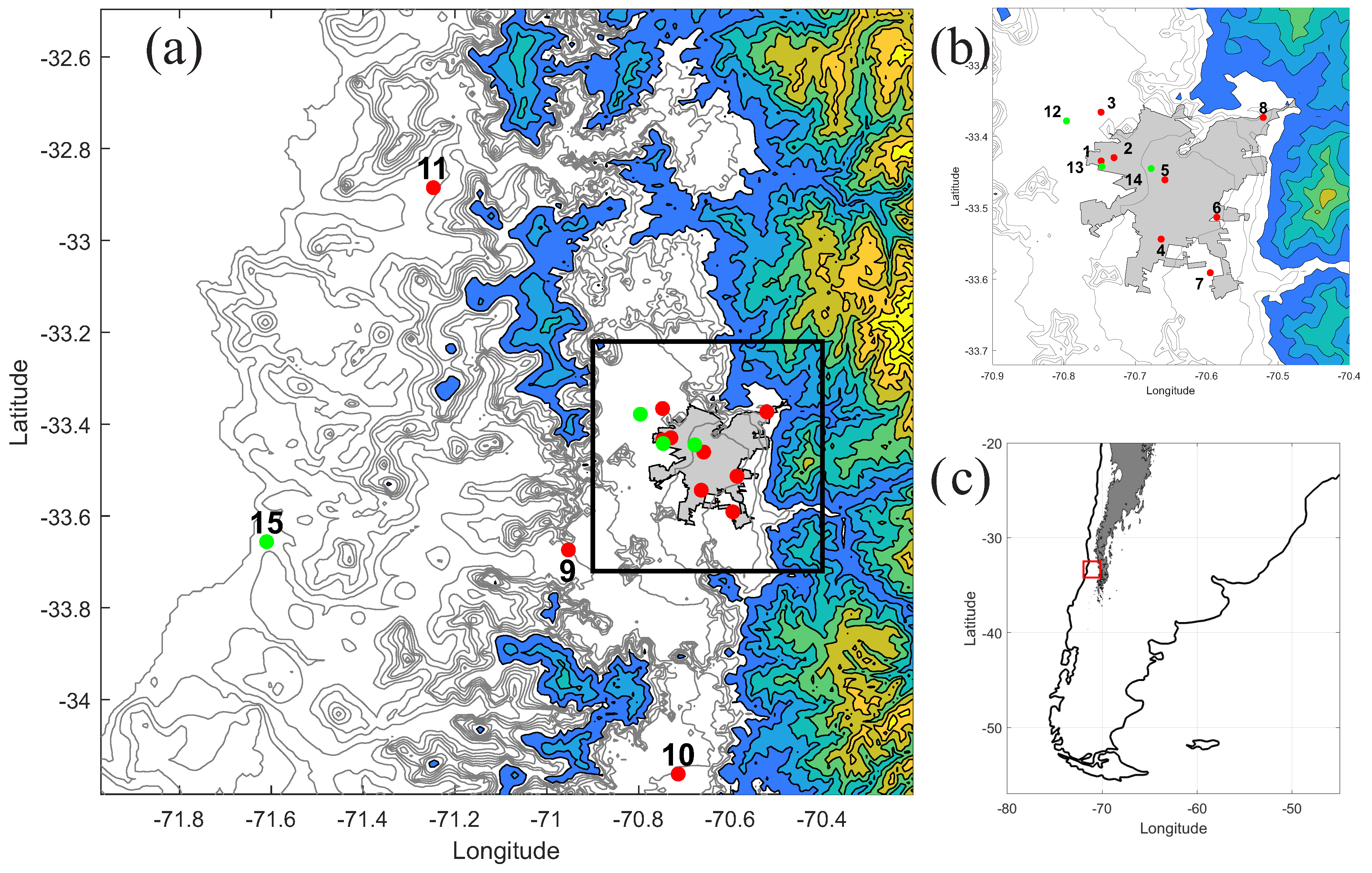
2. Materials and Methods

Figure 1 shows the location of points with the data used in this study. Sites 1 to 11 are air pollution monitoring stations operated by the Ministry of the Environment. Stations 1–8 are located in the urban area of Santiago, station 9 is in the southwestern entrance of the valley and stations 10 and 11 are located in contiguous valleys to the south and to the north of Santiago, respectively. The concentrations of PM₁₀ of stations 1 and 2 are used to compute the main pollution index in this study, because they are located in the area with highest concentrations and also because a similar index was used for the same purpose previously [13]. The other air pollution stations provide a means of assessing how representative this local index is of regional conditions. Points 12–15 in Figure 1 correspond to meteorological observation sites. Point 12 shows the location of the Santiago International Airport (SCEL) base operation site for the commercial airplanes providing the AMDAR vertical profiles of winds and temperature. Detailed description of the AMDAR data for Santiago, their validation and their use to estimate boundary layer heights based on Richardson number computation is presented in [22]. In particular, the comparison of AMDAR profiles with 33 morning radiosondes in Santiago showed almost perfect correlations for temperature and root mean squared deviations smaller than 1 °C in the vertical column below 4000 m AGL, while for winds above 1000 m AGL, correlation coefficients were larger than 0.7, and root mean squared deviations were smaller than 2 m s${}^{-1}$. Site 13 shows the location of the Department of Airfields and Aeronautical Services’ (DASA) 30 m micrometeorological tower, from which we use temperature measurements at 2 and 30 m AGL, as well as winds and turbulence data measured at 10 m AGL with an R. M. Young 81000 sonic anemometer [22]. Point 14 (Quinta Normal) is the main meteorological station in Santiago of the Chilean Weather Service, from which we obtain solar radiation data. Site 15 corresponds to the location of the Santo Domingo aerological station, where routine radiosondes are launched every day at 00 and 12 UTC (20 and 08 LT).

The PM${}_{10}$ hourly concentration averaged over stations 1 and 2 constitutes the main time series used in this work. As in [13], we restrict the analysis for the months from May to August, when PM air pollution in Santiago is worse. Only the years 2017–2019 are considered, because AMDAR data availability decreased substantially afterwards due to the pandemic and financial problems of the LATAM airline. The mean diurnal cycle of PM${}_{10}$ in Santiago shows marked peaks in the morning and evening hours [29]. Following [13], we define a daily PM index based on the PM${}_{10}$ concentrations averaged over hours 20–22 LT. The upper decile of this index defines a high-PM day. We perform our analysis in 3-day windows, selected by the condition that the central day (day D0) is a high-PM day, but the first day (day D−1) is not, so that the evolution of the meteorological conditions at the beginning of a PM episode are highlighted. Of the 25 episodes found, the third day of the window (day D+1) is also a high-PM day in 7 cases, but it is not in the remaining 18 cases.

Figure 2a shows the evolution of PM${}_{10}$ concentrations during the 3-day windows. The fine black line and the shading describe the mean and the upper and lower decile concentrations considering all days in the analysis period. The fine gray lines show the individual PM${}_{10}$ concentrations for the 25 selected episodes, while the bold black line shows their average. By definition, the episodes have significantly higher PM${}_{10}$ concentrations in hours 20–22 of day D0, although concentrations are higher than the average during all hours in days D0 and D+1. Despite being local in space and based upon just 3 h, Figure 2b shows that the pollution episodes defined with this methodology capture deficient air quality conditions over a much broader region. Indeed, for the majority of the monitoring stations shown in Figure 1, the 24 h mean PM${}_{10}$ concentrations of day D0 (right boxplots over each station in Figure 2b) are significantly higher than their overall averages (left boxplots over each station in Figure 2b). The only station in Santiago city not showing this behavior is station 8, whose altitude and eastward location make it less affected by the wintertime PM air pollution problem [30].

With the PM episodes defined as described above, the methodology reduces to computing the statistics of various meteorological variables conditioned by the occurrence of PM episodes and comparing them with their overall distributions. In particular, we show conditional diurnal cycles of surface temperature, stability, wind speed, vertical turbulence, surface sensible heat flux and global solar radiation. With the AMDAR profiles, we also examine the evolution of low-tropospheric temperature and wind anomalies during PM episodes, as well as the development of the boundary-layer height. The statistical significance of the differences between the conditional and overall averages is assessed with a Monte Carlo methodology: 1000 sets, consisting each one of 25 randomly-selected days, are subject to the same diagnostics (e.g., temperature diurnal cycle) as the set of 25 days corresponding to PM episodes. The diagnostics computed for PM episode days is then compared with the 10 and 90 percentile ranges of the 1000 random sets variability.

The local meteorological parameters described above are supplemented with a more regional view by considering the conditional statistics of the routine meteorological radiosondes at Santo Domingo and the meteorological fields provided by the ERA5 reanalysis [31]. In the Section 4, we argue that vertical subsidence plays a prominent role in the lower-tropospheric warming present during PM episodes. We use a thermodynamic method to estimate mean vertical velocity profiles from the AMDAR temperature and wind profiles using the methodology explained in Appendix A. These vertical velocity estimates are compared with ERA5 vertical velocity values averaged over the region between 33° S–34° S and 71° W–72° W (25 grid points). This averaging was needed to smooth out fine-scale variability in the vertical velocity field of the reanalysis, probably due to the complex terrain surrounding Santiago.

3. Results

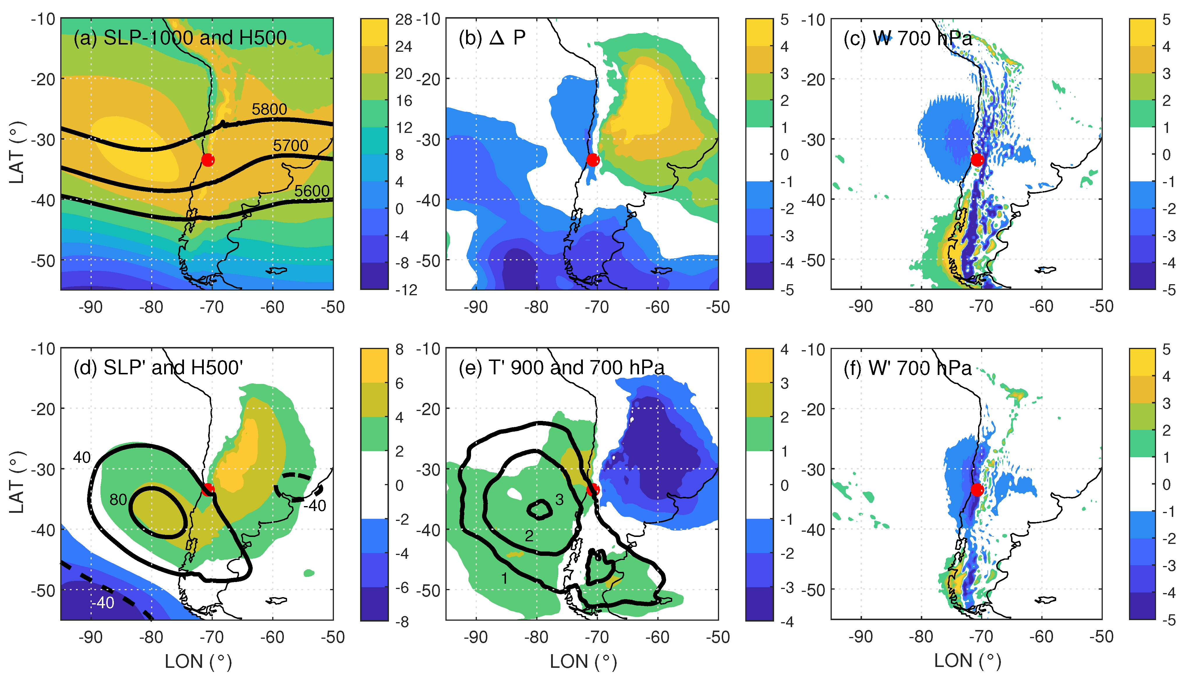
3.1. Synoptic-Scale Conditions

The synoptic-scale conditions associated with PM episodes are described based on the conditional averages of the reanalysis fields shown in the upper panels of Figure 3 (averages over days D0). Figure 3a shows the mean sea level pressure (SLP) field (colors) together with selected 500 hPa geopotential height contours. The latter depict a midtropospheric ridge with its axis off the Chilean coast, so that anticyclonic vorticity advection occurs at subtropical latitudes over the far-eastern Pacific and the west side of the continent. Consistently, the SLP field shows a strong subtropical high reaching into southcentral Chile and projecting to the east of the Andes. A trough in the SLP is present along the coast of northcentral Chile, extending down to the latitude of Santiago. These results are consistent with synoptic-scale features associated with air pollution events in Santiago and the attendant occurrence of coastal lows in this region [11,13]. The connection with coastal lows is also hinted at by a marked pressure drop along the coast of central Chile, shown in Figure 3b, in which averaged 24 h SLP changes (12 UTC pressure of day D0 minus 12 UTC pressure of day D−1) as large as −4 hPa are observed. Figure 3c shows intense lower-tropospheric subsidence off the coast of central Chile prevailing during the PM episodes.

The bottom panels in Figure 3 describe the anomaly represented by the conditions of PM episodes compared with the May–August fields averaged over the 3 years considered. Figure 3d shows that at 500 hPa, the ridge during PM episodes (Figure 3a) corresponds to an anticyclonic anomaly, inducing a southeasterly geostrophic wind anomaly above Santiago, which is later observed in the AMDAR wind profiles as well. At the surface, the positive anomaly in mean SLP takes a characteristic heart shape, with a western section very much in phase with the anticyclonic anomaly aloft, as well as an eastern section over Argentina with no anomaly signature aloft, pointing to the cold-core character of the high-pressure east of the Andes, seen in Figure 3a. Near Santiago, the pressure anomalies are very small, but they do not turn negative, probably because the subsynoptic scale of coastal lows can only marginally be represented with the 25 km resolution of the reanalysis. Figure 3e shows the temperature anomaly fields at 700 hPa (contours) and 900 hPa (colors). The high-pressure anomalies over Argentina are collocated with cold anomalies at low levels, signaling the occurrence of cold air surges to the east of the Andes (e.g., [32]). The ridge region off the Chilean coast is more or less in phase with a warm anomaly at 700 hPa. At 900 hPa, however, the maximum warm anomaly occurs close to the coast near Santiago, in association with the subsidence field at 700 hPa, evident in the PM episode averages (Figure 3c) and anomalies (Figure 3f).

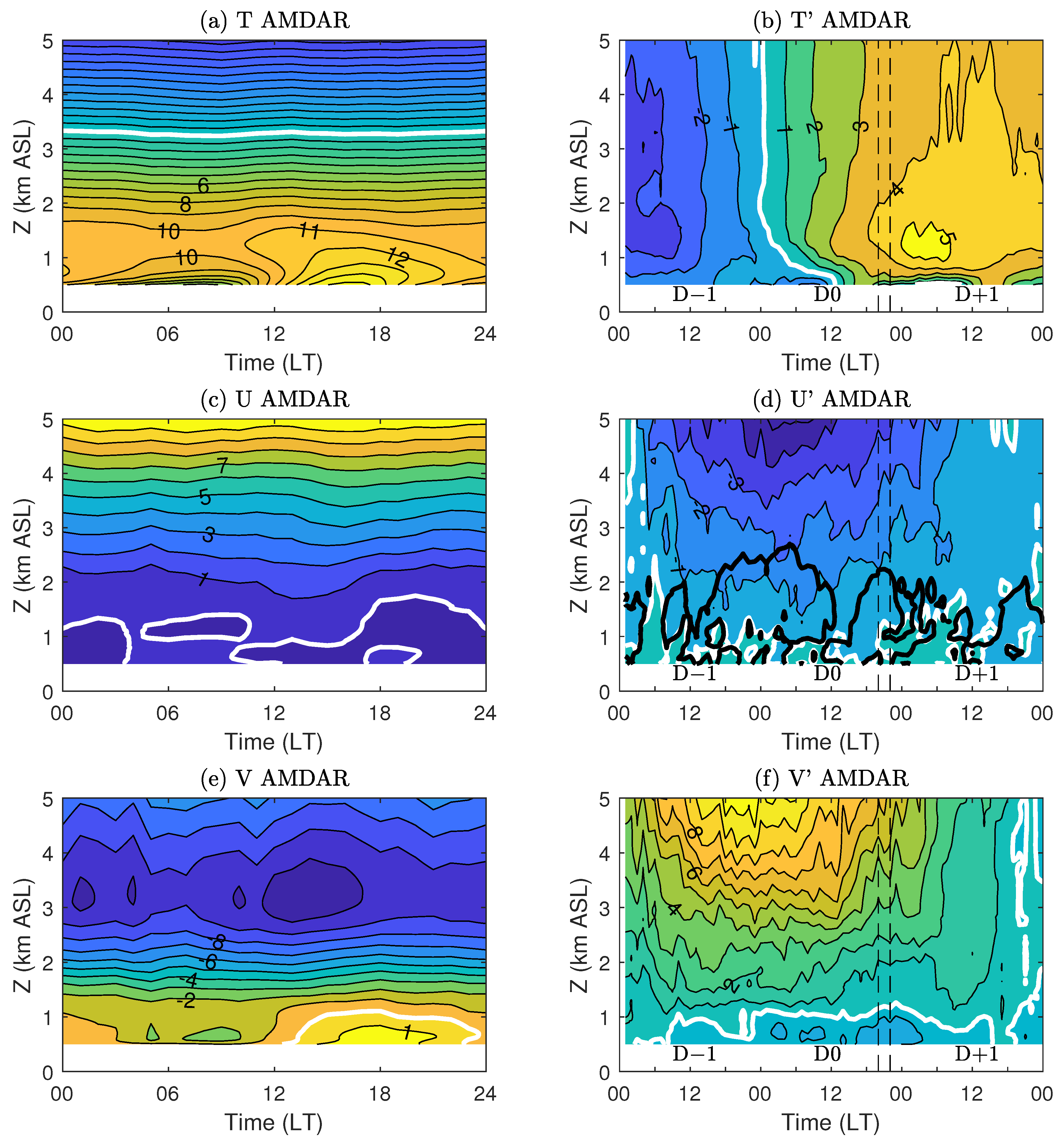
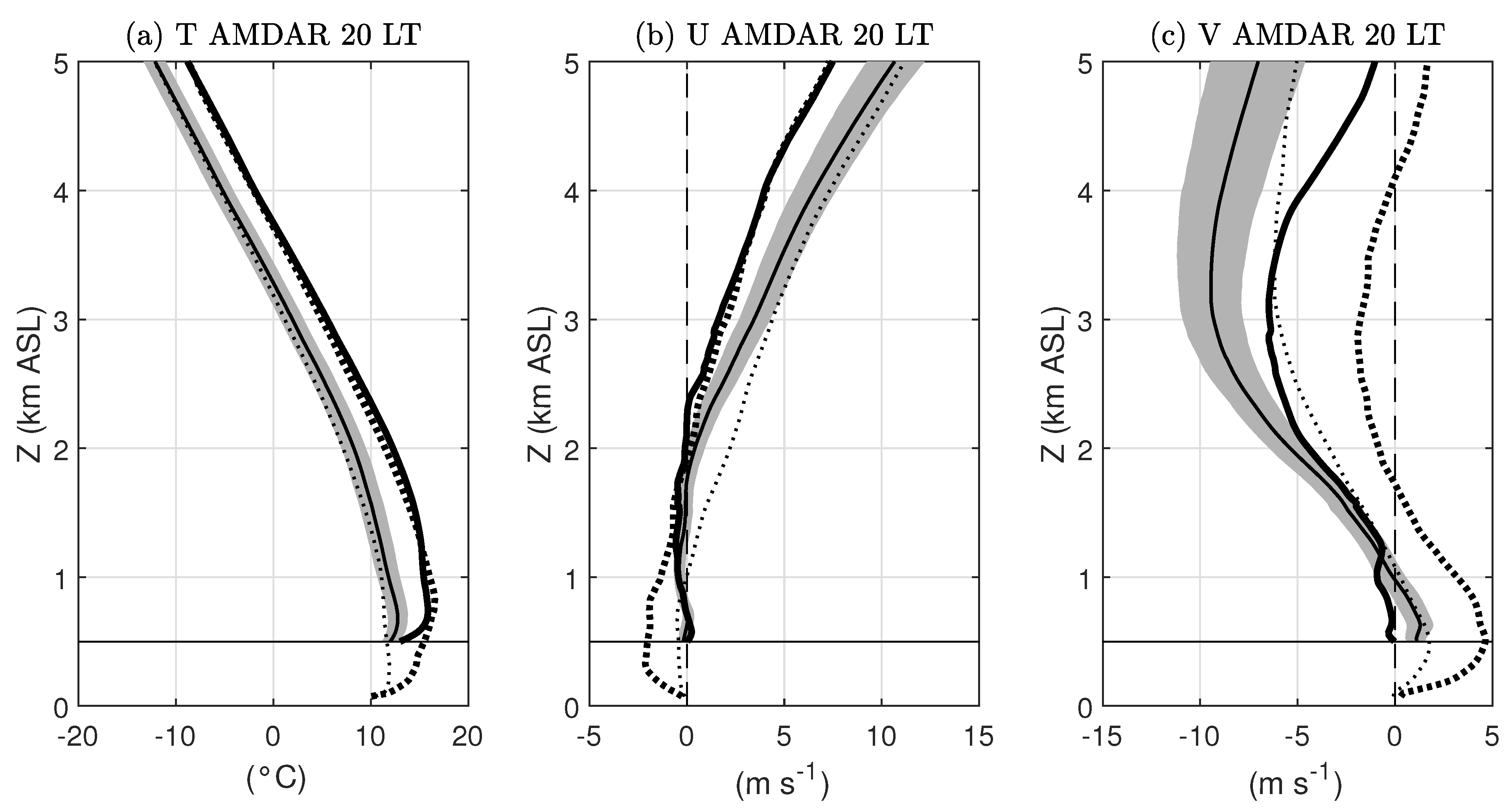
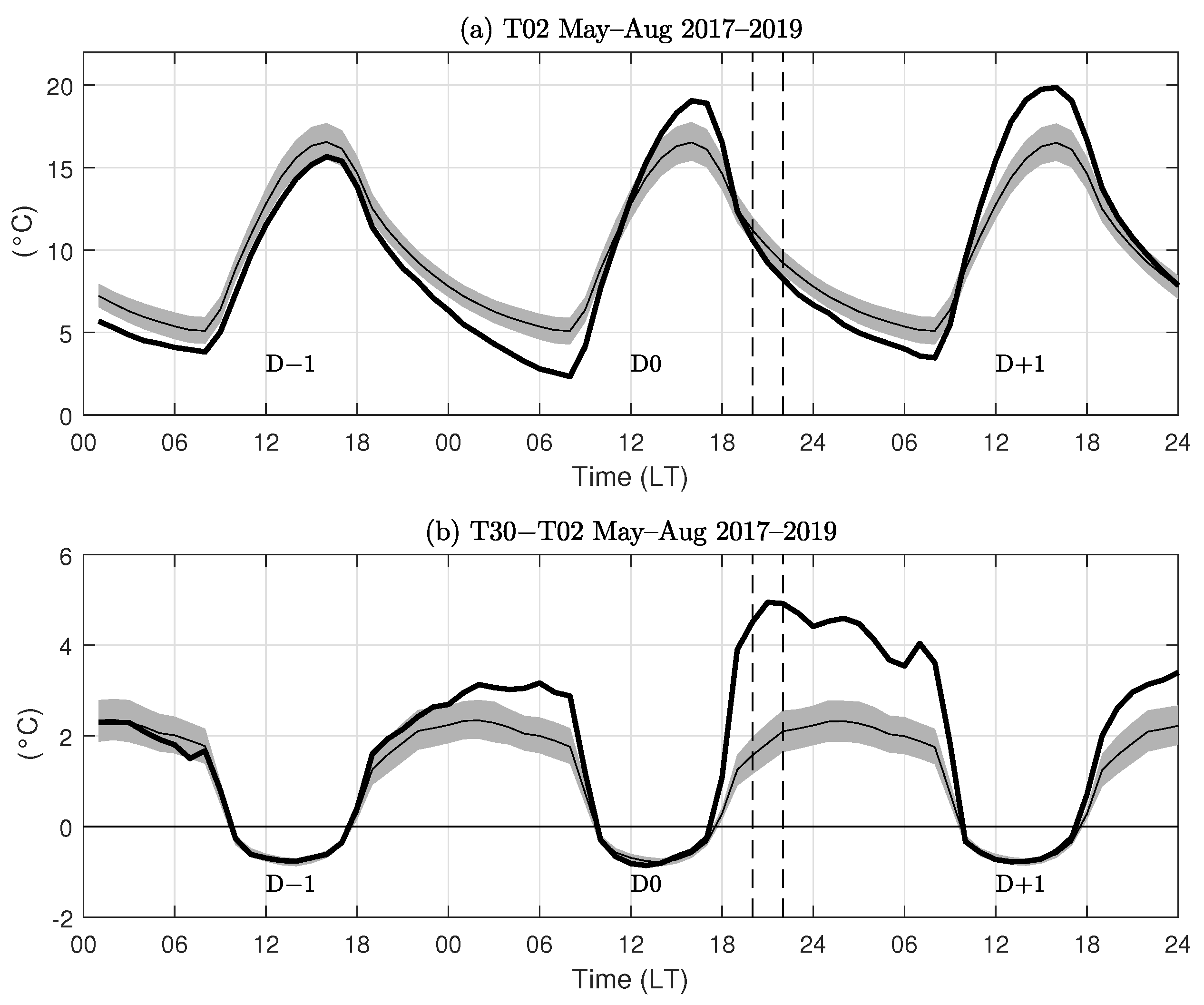
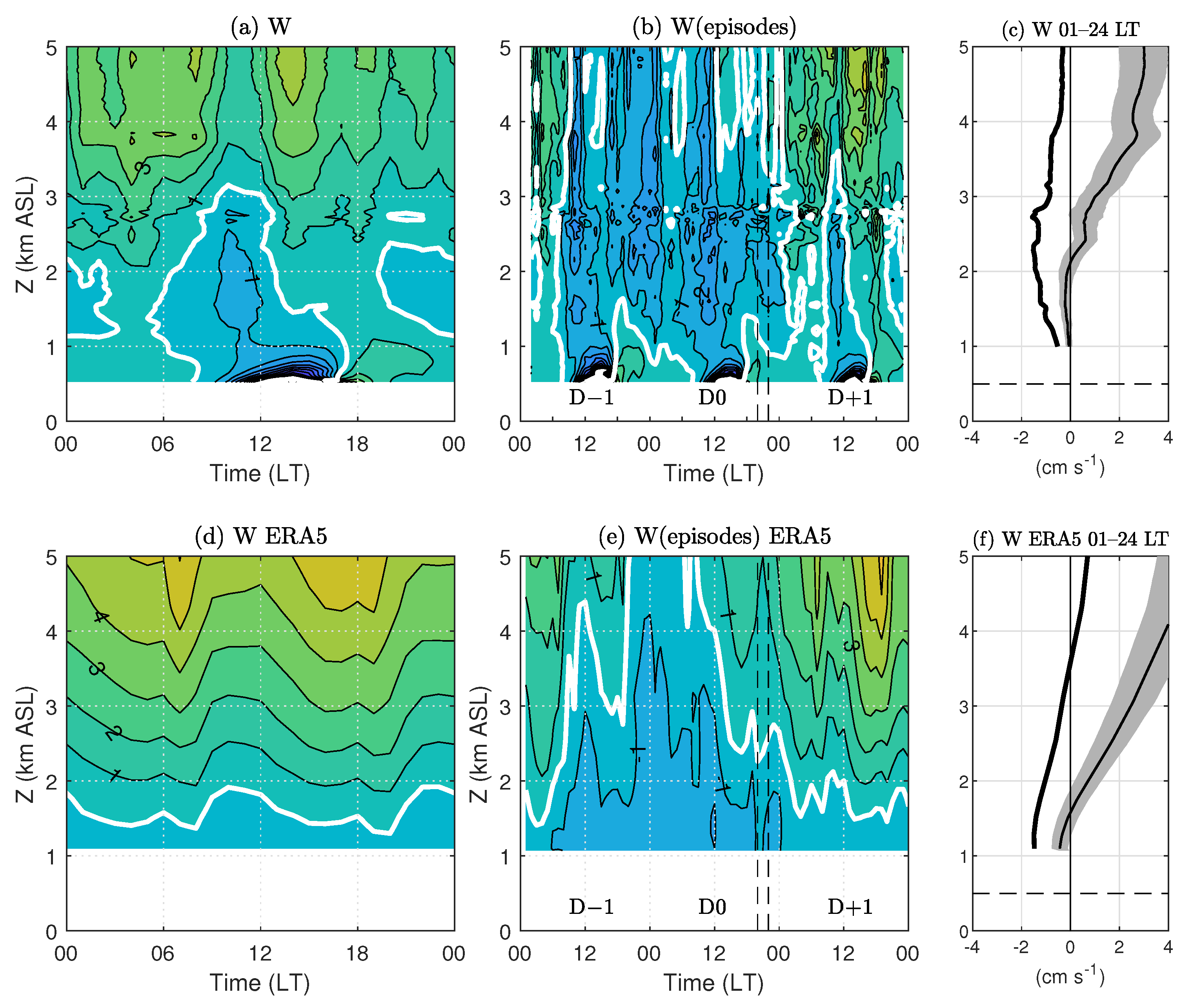
3.2. Vertical Conditions over the Valley

The AMDAR vertical profiles of temperature and wind allow an unprecedented description of the changes in the vertical structure of the lower troposphere during PM episodes (Figure 4). The left panels in Figure 4 show the mean diurnal cycles of these variables for the 500–5000 m ASL vertical range. The near-surface nocturnal cooling and the daytime warming of a 500–1000 m layer is clear in the temperature field (Figure 4a). Close to the surface, the mean winds have a weak easterly component and a southerly component that intensifies in the afternoon and evening hours. Aloft, the westerly winds increase steadily, while the meridional component defines a northerly jet centered about 3 km ASL, a feature attributed to the blocking of the westerlies by the Andes Cordillera [33,34]. The anomalies of these variables during PM episodes are shown for the 3-day window centered in day D0 in the right panels of Figure 4. A prominent warming of the full lower troposphere is evident in the temperature anomalies (Figure 4b). This warming is present during days D−1 and D0, reaching maximum values in the first hours of day D+1 at about 1.5 km ASL. In contrast, very near the surface, the temperature anomalies remain negative during the morning of day D0 and are smaller than the aloft ones during the afternoon of day D0 and the night of D+1, probably due to enhanced surface cooling associated with the clear sky conditions prevalent during PM episodes. As a result, the stability inside the valley increases strongly during the episodes.

In terms of winds, the overall anomalies during PM episodes correspond to a weakening of the zonal component (Figure 4d) and also of the meridional northerly wind (Figure 4f). These features are consistent with the midtropospheric ridge approaching central Chile, which was prevalent during the episodes (Figure 3a,d). The enhanced warming of the lower troposphere during coastal lows has been attributed to the easterly component of the winds that are forced to descend above the westerly slopes of the Andes [12], adding to the dynamic subsidence associated with the approaching synoptic ridge. Figure 4d indeed shows that during PM episodes, effective easterly winds prevail below 2 km during days D−1 and D0. In terms of the meridional component, we note the different signs in the anomalies close to the surface compared with the winds aloft. In particular, in the afternoon of day D0, the typical surface southerly winds show a negative anomaly, while the northerly jet aloft has a positive anomaly, resulting in a decrease in the meridional wind shear during the episodes.

To assess the significance of the anomalies described above, Figure 5 shows the AMDAR vertical profiles of temperature and wind components for hour 20 LT of day D0, including their overall Monte Carlo interdecile range and averages, as well as the means conditioned over PM episodes. The temperatures during PM episodes are significantly higher than the overall mean all over the column shown, with a shallow inversion near the surface. In the case of winds, the significance of the anomalies below 2 km ASL is hard to assess, because the magnitudes and variability are quite small, especially for the zonal component. To describe the regional reach of the AMDAR anomalies, we also plotted the mean profiles of the 20 LT (24 UTC) Santo Domingo soundings (fine dotted lines) and their averages conditioned over PM episodes (bold dotted lines) in Figure 5. The warming during PM episodes at Santo Domingo replicates what the AMDAR data show over the Santiago valley. The deep temperature inversion present at the coast in PM episodes extends from the surface up to about 800 m ASL. This feature reflects that during PM episodes, the subsidence inversion commonly observed in the Santo Domingo radiosondes is strong and deep, with its base reaching the surface and its top extending well above the altitude of the Santiago valley floor. With respect to the zonal wind, the Santo Domingo profile shows a clear easterly mean flow during PM episodes in the first kilometer above sea level, in contrast to the less distinct anomalies over the valley. The meridional component, on the other hand, shows positive anomalies all over the column during episodes, with a marked southerly low-level jet near the surface [35]. This contrasts with the change in sign of the meridional wind anomalies over the valley and the reduction in its southerly component near the surface.

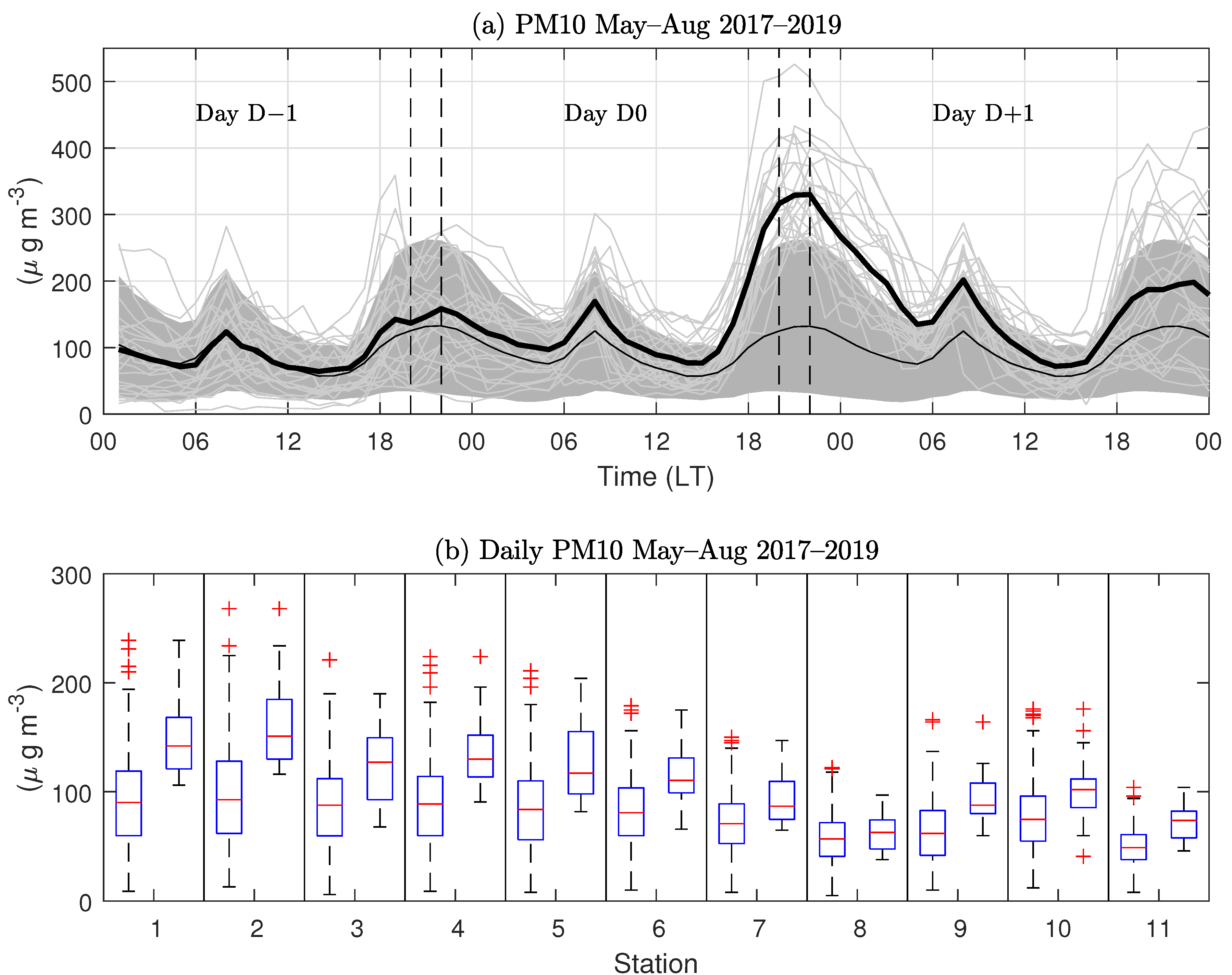
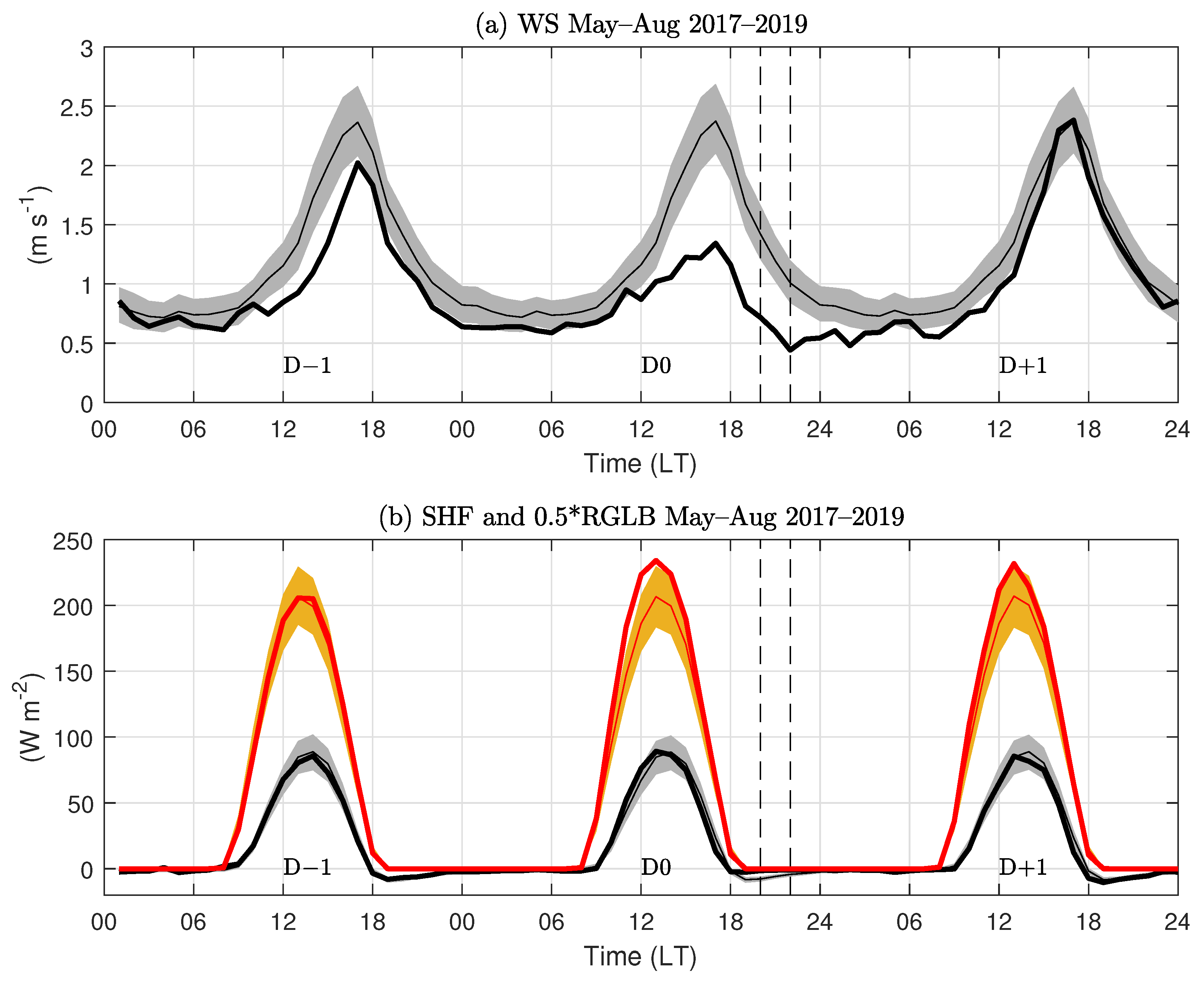
3.3. Surface Conditions in the Valley

The association between PM episodes and the temporal evolution of near-surface temperature and stability is shown in Figure 6. The results are consistent with what was shown by [13], namely a larger thermal amplitude during the day of the episode (day D0) and a significantly larger stability during the evening transition and the night. Both features tend to persist in day D+1, and the increased nocturnal stability is also present in day D−1, showing the multiday character of many of the PM episodes considered and their attendant synoptic-scale meteorological conditions.

Figure 7 extends the analysis to the surface wind speed and the turbulent sensible heat flux measured at the DASA tower. On day D0, wind speed is reduced compared with the overall diurnal cycle, being about half of the typical mean values during the afternoon and in the evening transition. In contrast, the mean daytime sensible heat flux shows no difference during the episodes compared with the overall averages. This result is intriguing, since PM episodes are typically clear days, as shown by the solar radiation diurnal cycles depicted in Figure 7b. Indeed, the mean solar radiation of PM episodes (day D0) extends above the 90 percentile range of this variable in the Monte Carlo ensembles. During the evening transition, on the other hand, the small negative values in sensible heat flux observed on average are much closer to zero during the PM episodes in association with the very weak nocturnal turbulent intensity described next.

Perhaps the two most relevant meteorological variables determining the vertical dispersion of air pollutants emitted near the surface are the intensity of the near-surface turbulence and the depth of the boundary layer. Based upon the new turbulent data from the DASA tower and the vertical profiles of the AMDAR observations, Figure 8 compares their mean evolution during PM episodes with their overall variation in the cold season.

The vertical turbulence intensity depicted in Figure 8a shows in general a marked diurnal cycle with maximum values in the afternoon and very low values at night. During PM episodes, the morning vertical turbulence is not very different from the overall averages, but a significant decrease occurs in the afternoon of D0, followed by a rapid drop towards negligible values in the evening transition and the subsequent night.

In terms of the ABL heights, Figure 8b shows that in the afternoon of D0, they are on average about 40% smaller than in the overall conditions (300 m versus 500 m). This daytime ABL height reduction occurring despite both sets of days having the same surface sensible heat flux (Figure 7b) is part of the discussion in Section 4. In the evening transition, the averaged ABL heights drop fast to very small values, showing that during PM episodes, the weaker turbulence is most of the time unable to produce unstable Richardson number values in the column, based on which the ABL heights were diagnosed using the AMDAR vertical profiles of temperature and winds [22].

4. Discussion

At the large and the small scales, our results confirm previous studies on the association between meteorological factors and the PM air pollution problem of Santiago. Indeed, our synoptic-scale fields for PM episodes (Figure 3) resemble the conditions identified by [13]: an elevated ridge approaching from the west, predominance of regional subsidence in the lower troposphere, a migratory surface high pressure moving eastwards to the south of central Chile and the development of a warm coastal trough in central Chile. At the smaller scale, the association of high surface PM concentrations in Santiago with increased surface stability, reduced wind speeds and turbulence documented here is consistent also with previous studies [13,20]. The added value of the present study is to use the new AMDAR data on valley-scale temperature and wind vertical profiles to examine the mechanisms linking these larger- and smaller-scale meteorological factors of the PM air pollution problem of Santiago, as discussed next.

4.1. Valley-Scale Stability and Subsidence

AMDAR data reveal that wind and temperature anomalies during PM episodes have a different vertical distribution. While easterly zonal wind anomalies and southerly meridional wind anomalies increase steadily with altitude in the 0–5000 m ASL layer shown in Figure 4, the temperature shows warming in the whole layer but with a maximum around 1.5 km ASL, thus significantly enhancing the vertical stability in the first 1000 m above the Santiago valley.

The role of subsidence in explaining the lower tropospheric warming during PM episodes is investigated by using the thermodynamic method mentioned in Section 2 and described in Appendix A. The three upper panels of Figure 9 show the inferred vertical velocity (W) fields. The overall diurnal cycle of W (Figure 9a) shows the layer above 3 km ASL, closer to the Andes ridge top, subject to mean ascent, while the layer between 1–2 km ASL has a semidiurnal variation with a very small averaged vertical velocity. In contrast, for the PM episodes (days D−1 and D0), the vertical velocity field below 5 km ASL is dominated by subsidence (Figure 9b), explaining much of the concomitant warming. Figure 9c shows the vertical profiles of the 24 h mean W values for day D0 and for the overall mean conditions, highlighting the statistically significant (i.e., outside the 10–90% interval in the frequency distribution) enhancement of the subsidence in the 2–3 km ASL layer during PM episodes.

To validate the vertical velocity inferred from the AMDAR data, the bottom panels in Figure 9 show the corresponding fields obtained from the ERA5 reanalysis. Naturally, the reanalysis W fields are smoother than those derived from observations, but they share similar patterns: overall averages that are positive, increase with altitude and show a marked semidiurnal oscillation (Figure 9d), while for PM episodes, the predominance of subsidence below 4–5 km ASL (Figure 9e,f) is also reproduced in the ERA5 W field.

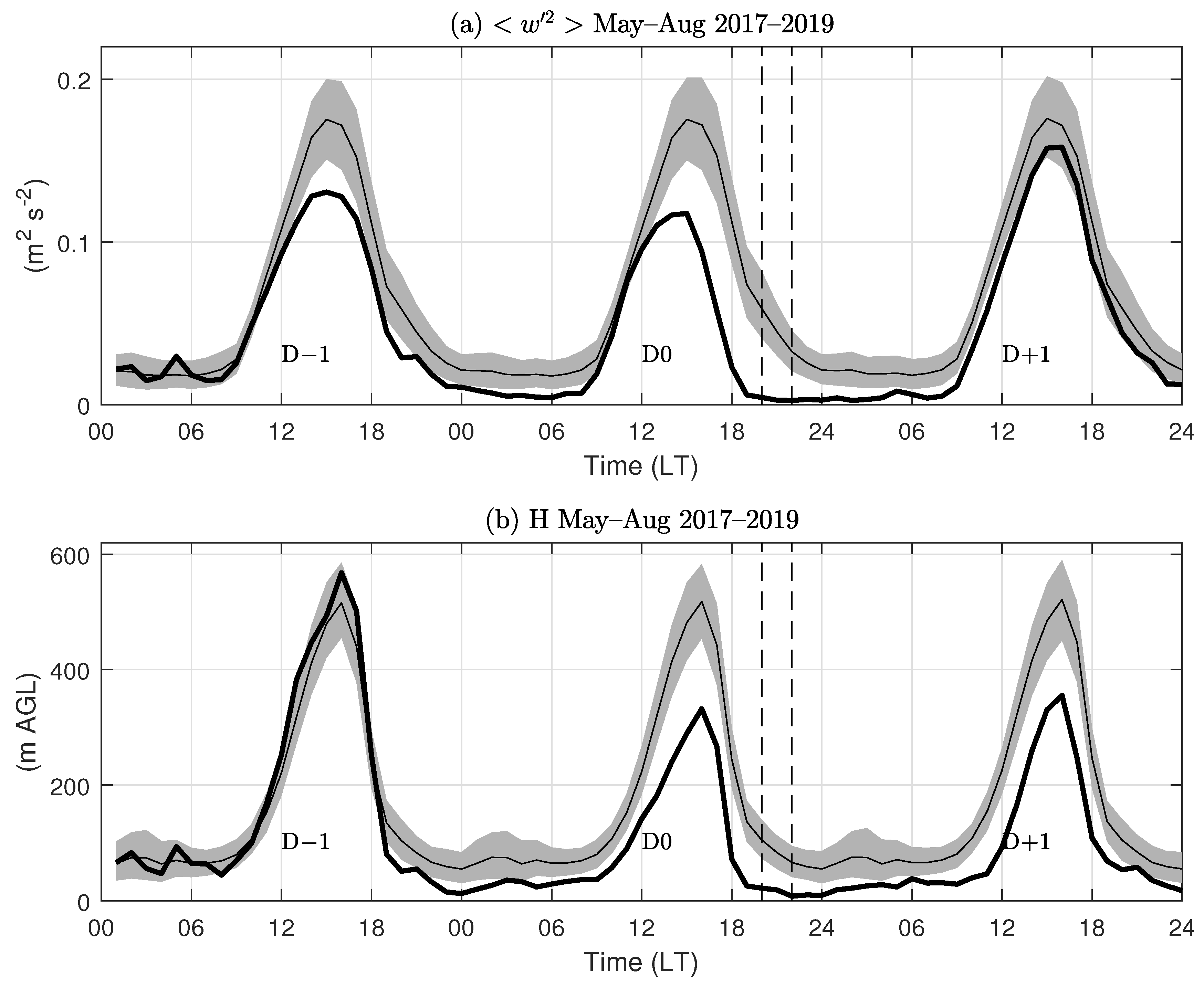
4.2. Daytime ABL Depth and the Surface Energy Budget

The increased subsidence in the lower troposphere and the enhanced valley-scale stability have a large impact on the development of the daytime ABL during PM episodes. The most direct effect is in the daytime ABL depth, which on day D0 of episodes reached a maximum typical value of 300 m compared with 500 m in the overall averages (Figure 8b). With both sets of days having the same sensible heat fluxes at the surface (Figure 7b), the difference is probably due to the regional subsidence during PM episodes. Indeed, the ∼0.7 cm s${}^{-1}$ mean subsidence rate existing during PM episodes at 1.5 km ASL (Figure 9c) acting over a 6 h period would induce a 150 m descent of the ABL depth, close to the 200 m ABL depth reduction actually observed.

In turn, the shallower ABL depths explain the larger surface thermal amplitude of PM episodes compared with the overall averages (Figure 6a), again considering both sets of days having the same surface sensible heat flux. A simple energy budget analysis of a convective ABL suggests that for constant surface sensible heat, the product $H_{\max }\Delta T_{\max }$ is approximately constant, where $H_{\max }$ is the maximum ABL depth in the afternoon and $\Delta T_{\max }$ is the maximum surface thermal amplitude [36]. Using values obtained from Figure 6a,b, we estimate $H_{\max }\Delta T_{\max }$ to be about 5000 K m and 5500 K m for the PM episodes and the overall conditions, respectively, which within 10% and as a first-order approach support the constant sensible heat flux assumption.

It is nevertheless curious that PM episodes have surface sensible heat fluxes that are similar to those of the overall conditions, considering that solar radiation reaching the surface is appreciably larger (Figure 7b). Our hypothesis is that the surplus of solar radiation during PM episodes is accounted for by the energy supporting the increased thermal amplitude of the near-surface soil layer in consonance with the larger thermal amplitude of the 2 m temperature discussed above. Verification of this, however, demands a more detailed analysis of the valley heat budget through modeling or more comprehensive observations, which falls beyond the scope of the present work.

4.3. Turbulence Intensity and Surface Winds

Compared with the overall conditions, the intensity of near-surface vertical turbulence shows minor differences during the morning of day D0 but a significant drop in the afternoon and negligible values in the evening transition and subsequent nocturnal conditions (Figure 8a). This collapse of the turbulence appears to be a main meteorological factor of the high PM concentrations reached during episodes.

In general, vertical turbulence is controlled by mechanical and buoyant factors. The former is commonly described by the wind shear, and the latter by the sensible heat flux or the stability of the temperature profile. In the afternoon of day D0, the drop in turbulence intensity appears to follow a decrease in surface winds (Figure 7a), pointing to the importance of mechanical turbulence generation at this time. In the evening and nocturnal conditions, weaker winds combined with increased stability (Figure 6b) almost entirely suppress the near-surface turbulence. This latter condition can be quantified by evaluating a bulk Richardson number defined by

$${\mathrm{Ri}}_b=\frac{g}{T}\frac{\Delta T}{\Delta Z_T}\frac{Z_V^2}{V^2},$$

(1)

where $\Delta T$ is the temperature difference measured over a depth $\Delta Z_T$, V is the wind speed measured at height $Z_V$, g is the acceleration of gravity and T is a mean temperature. In our case, we consider $\Delta Z_T=28$ m, $Z_V=10$ m, $g=9.8$ m s${}^{-2}$ and $T=283$ K. For evening and nocturnal conditions, the stability and wind speeds are obtained from Figure 6a and Figure 7a. Pairs $(\Delta T,V)$ are approximately (4 K, 0.5 m s${}^{-1}$) and (2 K, 1 m s${}^{-1}$) for PM episodes and overall conditions, respectively, resulting in Richardson numbers around 2 and 0.25 in each case. The latter value is typically considered as the upper threshold supporting turbulence in stable conditions [37]. The much larger Richardson value for PM episodes, on the other hand, explains the near-total annihilation of surface turbulence and the collapse of the nocturnal ABL depth during PM episodes.

Causes for the very weak surface winds in the afternoon and evening transition of PM episodes are discussed in connection to three mechanisms: entrainment of momentum from above the ABL, horizontal advection and the thermal forcing of the valley wind system. Figure 4e shows that typical afternoon winds inside and above the ABL have opposite directions. During PM episodes, the northerly winds above the ABL decrease, which through entrainment at the ABL top would enhance the southerly near-surface winds. Since this does not happen, entrainment of momentum appears not to produce the weakening of surface winds. Horizontal advection of the southerly winds prevailing at the coast is also discarded, because during PM episodes, the latter increase instead of decreasing (Figure 5c). Finally, considering the surface afternoon winds in Santiago to be part of a valley wind system, their weakening would point to a decrease in the thermal forcing of such a system. As discussed before, however, the sensible heat at the surface is not very different in PM episodes compared with the overall cases. The daytime ABL depth, on the other hand, is much shallower in PM episodes, which could make the valley wind system to develop in a much more confined topographic setting, thus restricting its intensity. Alternatively, the pressure reduction at the coast during PM episodes (Figure 3b) may be partially canceling the pressure gradient driving the afternoon winds in the valley. Additional factors like, for example, the impact of the aerosol load in the stability of the ABL (e.g., [38]) cannot be ruled out. These hypotheses can be tested in the future by numerical modeling of the Santiago valley wind system and evaluation of its sensitivity to topographic features.

5. Conclusions

We documented the local meteorological conditions associated with wintertime PM episodes in Santiago valley through the analysis of recently available observations, namely near-surface stability and turbulence measured in a 30 m tower and vertical profiles of wind and temperature registered by commercial airplanes operating at the Santiago airport (AMDAR database). This study illustrates the great potential that the relatively new AMDAR data have in bridging the observational gap between large-scale conditions (commonly diagnosed with reanalysis fields) and local measurements performed near the surface. The semicontinuous availability of vertical profiles of temperature and winds provided by the AMDAR database near busy airports offers the opportunity of a detailed characterization of the lower troposphere and the ABL, with applications, for example, in air pollution problems.

The regional context of the study was provided by considering the high-resolution ERA5 reanalysis fields. The results associate the PM episodes with a midtropospheric ridge approaching central Chile, a drop in surface pressure at the coast and strengthened subsidence in the lower troposphere. These regional features are consistent with what previous studies have shown about the synoptic forcings of the wintertime air pollution problem of Santiago [13].

Our analysis of AMDAR data shows that the regional subsidence prevalent during PM episodes is responsible of a significant lower-tropospheric warming that maximizes around 1.5 km ASL, thus greatly increasing the valley-scale stability. In turn, during daytime of PM episodes, this larger stability significantly reduces the ABL depth and increases the daytime surface thermal amplitude, effects that are consistent with a surface sensible heat flux that does not vary appreciably, which is confirmed by the available turbulence measurements and the computation of a simple heat budget of the convective ABL.

During the evening transition of PM episodes, the vertical turbulence intensity decreases along with the reduction in surface winds. Later in the night, a Richardson number analysis shows that the enhanced near-surface stability and the weaker winds are unable to maintain turbulent conditions, which is consistent with the near-zero values of vertical velocity variance and PBL depth measured at these hours. The physical mechanism explaining the weaker winds during PM episodes is not clear yet, and we postulate that the shallower ABL depth restricts the intensity of the valley wind system, which may be tested in the future with numerical modeling of the ABL dynamics in the Santiago valley.

The new data analyzed here, especially the AMDAR data, allowed us to link the large-scale conditions known to exist during PM episodes in Santiago with the local meteorological factors affecting the dispersion of air pollutants, namely turbulence intensity and ABL depth. The analysis shows the physical mechanisms behind this linkage and also provides a basis for a more comprehensive validation of mesoscale numerical models used in representing these processes, ultimately applied in the management and forecasting of the air pollution problem of Santiago.

References

1. Koutrakis, P.; Sax, S.N.; Sarnat, J.A.; Coull, B.; Demokritou, P.; Oyola, P.; García, J.; Gramsch, E. Analysis of PM10, PM2.5, and PM2.5–10 concentrations in Santiago, Chile, from 1989 to 2001. J. Air Waste Manag. Assoc. 2005, 55, 342–351. [Google Scholar] [CrossRef]
2. Carbone, S.; Saarikoski, S.; Frey, A.; Reyes, F.; Reyes, P.; Castillo, M.; Gramsch, E.; Oyola, P.; Jayne, J.; Worsnop, D.R.; et al. Chemical characterization of submicron Aerosol particles in Santiago de Chile. Aerosol. Air Qual. Res. 2013, 13, 462–473. [Google Scholar] [CrossRef]
3. Gallardo, L.; Barraza, F.; Ceballos, A.; Galleguillos, M.; Huneeus, N.; Lambert, F.; Ibarra, C.; Munizaga, M.; Osses, M.; Tolvett, S.; et al. Evolution of air quality in Santiago: The role of mobility and lessons from the science-policy interface. Elem. Sci. Anthr. 2018, 6, 38. [Google Scholar] [CrossRef]
4. Cifuentes, L.A.; Vega, J.; Kopfer, K.; Lava, L.B. Effect of the fine fraction of particulate matter versus the coarse mass and other pollutants on daily mortality in Santiago, Chile. J. Air Waste Manag. Assoc. 2000, 50, 1287–1298. [Google Scholar] [CrossRef] [PubMed]
5. Leiva, M.A.; Santibañez, D.A.; Ibarra, S.; Matus, P.; Seguel, R. A five-year study of particulate matter (PM2.5) and cerebrovascular diseases. Environ. Pollut. 2013, 181, 1–6. [Google Scholar] [CrossRef] [PubMed]
6. Barraza, F.; Lambert, F.; Jorquera, H.; Villalobos, A.M.; Gallardo, L. Temporal evolution of main ambient PM2.5 sources in Santiago, Chile, from 1998 to 2012. Atmos. Chem. Phys. 2017, 17, 10093–10107. [Google Scholar] [CrossRef]
7. Mullins, J.; Bharadwaj, P. Effects of Short-Term Measures to Curb Air Pollution: Evidence from Santiago, Chile. Am. J. Agricul. Econ. 2015, 97, 1107–1134. [Google Scholar] [CrossRef]
8. Gramsch, E.; Oyola, P.; Reyes, F.; Rojas, F.; Henríquez, A.; Kang, C.M. Trends in particle matter and its elemental composition in Santiago de Chile, 2011–2018. J. Air Waste Manag. Assoc. 2021, 71, 721–736. [Google Scholar] [CrossRef]
9. Jorquera, H. Ambient particulate matter in Santiago, Chile: 1989–2018: A tale of two size fractions. J. Environ. Manag. 2020, 258, 110035. [Google Scholar] [CrossRef] [PubMed]
10. Falvey, M.; Garreaud, R. Wintertime Precipitation Episodes in Central Chile: Associated Meteorological Conditions and Orographic Influences. J. Hydrometeorol. 2007, 8, 171–193. [Google Scholar] [CrossRef]
11. Rutllant, J.; Garreaud, R. Meteorological air pollution potential for Santiago, Chile: Towards an objective episode forecasting. Environ. Monitor. Assess. 1995, 34, 223–244. [Google Scholar] [CrossRef] [PubMed]
12. Garreaud, R.; Rutllant, J.; Fuenzalida, H. Coastal lows along the subtropical west coast of South America: Mean structure and evolution. Mon. Weather Rev. 2002, 130, 75–88. [Google Scholar] [CrossRef]
13. Garreaud, R.; Rutllant, J. Meteorological factors of the air pollution in Santiago (in Spanish). In Critical Episodes of Air Pollution in Santiago; Morales, R., Ed.; Editorial Universitaria: Santiago, Chile, 2006; pp. 36–53. [Google Scholar]
14. Saide, P.E.; Carmichael, G.R.; Spak, S.N.; Gallardo, L.; Osses, A.; Mena-Carrasco, M.; Pagowski, M. Forecasting urban PM10 and PM2.5 pollution episodes in very stable nocturnal conditions and complex terrain using WRF-Chem CO tracer model. Atmos. Environ. 2011, 45, 2769–2780. [Google Scholar] [CrossRef]
15. Saide, P.E.; Mena-Carrasco, M.; Tolvett, S.; Hernandez, P.; Carmichael, G.R. Air quality forecasting for winter-time PM2.5 episodes occurring in multiple cities in central and southern Chile. J. Geophys. Res. 2016, 121, 558–575. [Google Scholar] [CrossRef]
16. Garreaud, R.; Rutllant, J. Coastal lows in north-central Chile: Numerical simulation of a typical case. Mon. Weather Rev. 2003, 131, 891–908. [Google Scholar] [CrossRef]
17. Morales-Solís, K.; Ahumada, H.; Rojas, J.P.; Urdanivia, F.R.; Catalán, F.; Claramunt, T.; Toro, R.A.; Manzano, C.A.; Leiva-Guzmán, M.A. The Effect of COVID-19 Lockdowns on the Air Pollution of Urban Areas of Central and Southern Chile. Aerosol Air Qual. Res. 2021, 21, 200677. [Google Scholar] [CrossRef]
18. Chen, J.; Yin, D.; Zhao, Z.; Kaduwela, A.; Avise, J.; DaMassa, J.; Beyersdorf, A.; Burton, S.; Ferrare, R.; Herman, J.; et al. Modeling air quality in the San Joaquin valley of California during the 2013 Discover-AQ field campaign. Atmos. Environ. X 2020, 5, 100067. [Google Scholar] [CrossRef]
19. Li, X.; Xia, X.; Wang, L.; Cai, R.; Zhao, L.; Feng, Z.; Ren, Q.; Zhao, K. The role of foehn in the formation of heavy air pollution events in Urumqi, China. J. Geophys. Res. Atmos. 2015, 120, 5371–5384. [Google Scholar] [CrossRef]
20. Muñoz, R.; Corral, M. Surface Indices of Wind, Stability, and Turbulence at a Highly Polluted Urban Site in Santiago, Chile, and their Relationship with Nocturnal Particulate Matter Concentrations. Aerosol Air Qual. Res. 2017, 17, 2780–2790. [Google Scholar] [CrossRef]
21. Moninger, W.R.; Mamrosh, R.D.; Pauley, P.M. Automated meteorological reports from commercial aircraft. Bull. Am. Meteorol. Soc. 2003, 84, 203–216. [Google Scholar] [CrossRef]
22. Muñoz, R.; Whiteman, C.D.; Garreaud, R.; Rutllant, J.; Hidalgo, J. Using Commercial Aircraft Meteorological Data to Assess the Heat Budget of the Convective Boundary Layer over the Santiago Valley in Central Chile. Boun. Layer Met. 2022, 183, 295–319. [Google Scholar] [CrossRef]
23. Cardinali, C.; Isaksen, L.; Andersson, E. Use and impact of automated aircraft data in a global 4DVAR data assimilation system. Mon. Weather Rev. 2003, 131, 1865–1877. [Google Scholar] [CrossRef]
24. Petersen, R.A. On the impact and benefits of AMDAR observations in operational forecasting. Part I: A review of the impact of automated aircraft wind and temperature reports. Bull. Am. Meteorol. Soc. 2016, 97, 585–602. [Google Scholar] [CrossRef]
25. Zhang, Y.; Sun, K.; Gao, Z.; Pan, Z.; Shook, M.A.; Li, D. Diurnal climatology of planetary boundary layer height over the contiguous United States derived from AMDAR and reanalysis data. J. Geophys. Res. 2020, 125, e2020JD032803. [Google Scholar] [CrossRef]
26. Rahn, D.A.; Mitchell, C.J. Diurnal climatology of the boundary layer in southern California using AMDAR temperature and wind profiles. J. Appl. Meteorol. Climatol. 2016, 55, 1123–1137. [Google Scholar] [CrossRef]
27. Pérez, I.; García, M.; Sánchez, M.; Pardo, N.; Fernández-Duque, B. Key Points in Air Pollution Meteorology. Int. J. Environ. Res. Public Health 2020, 17, 8349. [Google Scholar] [CrossRef] [PubMed]
28. Zhang, Y. Seasonal Disparity in the Effect of Meteorological Conditions on Air Quality in China Based on Artificial Intelligence. Atmosphere 2021, 12, 1670. [Google Scholar] [CrossRef]
29. Muñoz, R. Relative roles of emissions and meteorology in the diurnal pattern of urban PM10: Analysis of the daylight saving time effect. J. Air Waste Manag. Assoc. 2012, 62, 642–650. [Google Scholar] [CrossRef]
30. Gramsch, E.; Cereceda-Balic, F.; Oyola, P.; von Baer, D. Examination of pollution trends in Santiago de Chile with cluster analysis of PM10 and Ozone data. Atmos. Environ. 2006, 40, 5464–5475. [Google Scholar] [CrossRef]
31. Hersbach, H.; Bell, B.; Berrisford, P.; Hirahara, S.; Horányi, A.; Muñoz-Sabater, J.; Nicolas, J.; Peubey, C.; Radu, R.; Schepers, D.; et al. The ERA5 global reanalysis. Quart. J. R. Meteor. Soc. 2020, 146, 1999–2049. [Google Scholar] [CrossRef]
32. Garreaud, R. Cold air incursions over Subtropical South America: Mean structure and dynamics. Mon. Weather Rev. 2000, 128, 2544–2559. [Google Scholar] [CrossRef]
33. Rutllant, J.; Garreaud, R. Episodes of strong flow down the western slope of the subtropical Andes. Mon. Weather Rev. 2004, 132, 611–622. [Google Scholar] [CrossRef]
34. Scaff, L.; Rutllant, J.; Rahn, D.; Rondanelli, R.; Gascoin, S. Meteorological interpretation of orographic precipitation gradients along an Andes west slope basin at 30 S (Elqui valley, Chile). J. Hydromeorol. 2017, 18, 713–727. [Google Scholar] [CrossRef]
35. Garreaud, R.; Muñoz, R. The Low-Level Jet off the West Coast of Subtropical South America: Structure and Variability. Mon. Weather Rev. 2005, 133, 2246–2261. [Google Scholar] [CrossRef]
36. Stull, R. An Introduction to Boundary Layer Meteorology; Kluwer Academic Publishers: Dordrecht, The Netherlands, 1988; pp. 472–473. [Google Scholar]
37. Vila-Guerau, J.; van Heerwaarden, C.; van Stratum, B.; van den Dries, K. Atmospheric boundary layer. In Integrating Air Chemistry and Land Interactions; Cambridge University Press: New York, NY, USA, 2015; p. 68. [Google Scholar]
38. Su, T.; Li, Z.; Li, C.; Li, J.; Han, W.; Shen, C.; Tan, W.; Wei, J.; Guo, J. The significant impact of aerosol vertical structure on lower atmosphere stability and its critical role in aerosol–planetary boundary layer (PBL) interactions. Atmos. Chem. Phys. 2020, 20, 3713–3724. [Google Scholar] [CrossRef]
39. Holton, J. An Introduction to Dynamic Meteorology, 4th ed.; Elsevier Academic Press: Boston, MA, USA, 2004; p. 77. [Google Scholar]
40. Moeng, C.-H. Stratocumulus-topped atmospheric planetary boundary layer. In Buoyant Convection in Geophysical Flows; Plate, E.J., Fedorovich, E.E., Viegas, D.X., Wyngaard, J.C., Eds.; Kluwer: Dordrecht, The Netherlands, 1998; pp. 421–440. [Google Scholar]
Figure 1. (a) Topographic map of the Santiago valley and surroundings. Contour lines from 0 to 800 m ASL every 100 m. Shaded contours from 1000 to 5000 m ASL every 500 m. Black rectangle is zoomed in panel (b). (b) Zoom over the Santiago urban area (shaded). (c) Location of the study area (red square) in southern South America. Shading marks elevations greater than 3000 m ASL. In (a,b), red circles (1–11) mark sites of air quality monitoring stations and green circles mark sites with meteorological observations used in this work: 12: Santiago airport (SCEL), 13: DASA tower, 14: Quinta Normal weather station, 15: Santo Domingo aerological station.
Atmosphere 14 01454 g001
Figure 2. (a) Three-day diurnal cycles of PM 10  index for the period May–August 2017–2019. Shaded region shows 10–90 percentile regions of the data. Fine black line shows overall mean value and bold line the mean values of PM 10  episodes. Fine gray lines show PM 10  concentrations for the individual episode days corresponding to the central day of the 3-day window (day D0). Vertical dashed lines at hours 20, 22 of D0 mark the period defining the episodes. Vertical dashed lines at hours 20, 22 of day D−1 mark the same hours of the previous day. (b) Frequency distributions of daily PM 10  concentrations for the 11 air quality stations shown in Figure 1. Left boxes show distributions of all May–August days and right boxes are restricted over PM 10  episode days. Box limits correspond to the upper and lower quartiles of the distributions, the red line marks the median and red crosses mark outlier values.
Atmosphere 14 01454 g002
Figure 3. ERA5 fields averaged over PM episodes: (a) Sea level pressure minus 1000 hPa (colors; hPa) and 500 hPa heights (contours; m), (b) 24 h sea level pressure change (hPa), (c) 700 hPa vertical velocity (cm s 1 ). Anomalies with respect to May–August averages: (d) Sea level pressure (colors; hPa) and 500 hPa heights (contours; m), (e) temperature (°C) at 900 hPa (colors) and 700 hPa (contours) and (f) 700 hPa vertical velocity (cm s 1 ).
Atmosphere 14 01454 g003
Figure 4. (a) Height–time diurnal cycles of temperature (°C) averaged over the full May–August period. (b) Three-day anomalies of temperature (°C) of PM episodes around day D0. (c) As (a) but for zonal wind speed (m s 1 ). (d) As (b) but for zonal wind speed (m s 1 ). (e) As (a) but for meridional wind speed (m s 1 ). (f) As (b) but for meridional wind speed (m s 1 ). White lines mark the zero values. In (d), the black contour surrounds the region with negative mean zonal winds.
Atmosphere 14 01454 g004
Figure 5. Vertical profiles of meteorological variables at 20 LT: (a) temperature, (b) zonal wind and (c) meridional wind. Fine lines mark AMDAR averages for May–August. Bold lines are the average of the 25 days defined as PM episodes. Shading marks the 10 and 90 percentile regions of 1000 randomly generated 25-day sets. Fine and bold dotted lines show Santo Domingo averages for overall conditions and PM episodes, respectively.
Atmosphere 14 01454 g005
Figure 6. DASA tower observations: (a) surface temperature; (b) temperature difference between 30 m and 2 m levels. Fine lines mark averages for May–August. Bold lines are the average of the 25 days defined as PM episodes. Shading marks the 10 and 90 percentile regions of 1000 randomly generated 25-day sets.
Atmosphere 14 01454 g006
Figure 7. (a) Ten meter wind speed at DASA tower: (b) Sensible heat flux at DASA tower (black) and solar radiation at Quinta Normal station (orange). For better joint appreciation, the solar radiation is scaled by two.Fine lines mark averages for May–August. Bold lines are the average of the 25 days defined as PM episodes. Shading marks the 10 and 90 percentile regions of 1000 randomly generated 25-day sets.
Atmosphere 14 01454 g007
Figure 8. (a) Vertical velocity variance at DASA tower. (b) Boundary layer height derived from AMDAR observations. Fine lines mark averages for May–August. Bold lines are the average of the 25 days defined as PM episodes. Shading marks the 10 and 90 percentile regions of 1000 randomly generated 25-day sets.
Atmosphere 14 01454 g008
Figure 9. (a,d): height–time diurnal cycle of vertical velocity (cm s 1 ) averaged over May–August. (b,e): 3-day variation in vertical velocity averaged over PM episodes. White contours mark zero values. (c,f): vertical profiles of 24 h mean vertical velocity averaged over May–August (fine line) and over PM episodes (bold line). Shading marks the 10 and 90 percentile regions of 1000 randomly generated 25-day sets. In the upper (lower) panels, vertical velocity is inferred from AMDAR data (ERA5 reanalysis).
Atmosphere 14 01454 g009
Disclaimer/Publisher’s Note: The statements, opinions and data contained in all publications are solely those of the individual author(s) and contributor(s) and not of MDPI and/or the editor(s). MDPI and/or the editor(s) disclaim responsibility for any injury to people or property resulting from any ideas, methods, instructions or products referred to in the content.