Ionospheric Variations Induced by Thunderstorms in the Central Region of Argentina during the RELAMPAGO–CACTI Campaign

Abstract

The ionosphere can be perturbed by solar and geomagnetic activity, earthquakes, thunderstorms, etc. In particular, electromagnetic pulses produced by thunderstorms can generate wave structures in the ionospheric plasma, which are known as atmospheric gravity waves (AGWs), which can be detected by measuring the total electron content (TEC). We studied ionospheric variations resulting from thunderstorms on 10 November 2018, between 00:00 and 08:00 UTC, in the central region of Argentina, site of the RELAMPAGO–CACTI Project (Remote sensing of Electrification, Lightning, and Mesoscale/Microscale Processes with Adaptive Ground Observations; Clouds, Aerosols, and Complex Terrain Interactions). Atmospheric electrical activity data were provided by the Earth Networks Total Lightning Network (ENTLN) and the TEC was computed from Global Navigation Satellite System (GNSS) measurements provided by the Argentinian Continuous Satellite Monitoring Network (RAMSAC by its Spanish acronym). We found AGWs with periods less than or equal to 100 min and peak-to-peak Differential Vertical Total Electron Content (DVTEC) amplitude values up to 1.35 TECU (1 total electron content unit $={10}^{16}$ electrons/m${}^2$). We observed that AGWs show the highest peak-to-peak amplitudes during intense thunderstorm periods. On a day without thunderstorms, the peak-to-peak amplitudes were approximately 2.91 times lower.

1. Introduction

The ionosphere is the region of the atmosphere constituted by the presence of ions and free electrons. It extends mainly between 60 km and 1000 km [1] above the Earth’s surface, and solar radiation is its principal ionization agent [2]. Through Global Navigation Satellite System (GNSS) measurements, the total electron content (TEC) can be calculated. TEC is defined as the integrated electron density along the signal path from the satellite to the GNSS receiver [3]. This can be dynamically perturbed by external influences, such as solar activity and geomagnetic storms, among others; and by internal influences, such as thunderstorms, earthquakes, etc. [4].

Regarding internal influences, thunderstorms, and convective systems can generate wave structures in the ionospheric plasma [3,5,6]. These structures, known as atmospheric gravity waves (AGWs), have been related to electromagnetic pulses during thunderstorms [7], and they can also be detected by GNSS measurements [8]. Overshooting top, lightning, or a combination of both can generate gravity waves [3,9]. Transient Luminous Events (TLEs) and discharges originating in the stratiform region could be a source of these waves [10,11].

AGWs can propagate vertically upwards and transfer energy and momentum to the ionosphere [1]. As they ascend, they can become unstable and break up, generating secondary waves [12]. These secondary waves on their journey modulate the ionospheric plasma in the E region [12].

Vadas, S. L. and Liu, H. L. 2009 [13] analyzed the response of the thermosphere and ionosphere to the dissipation of gravity waves excited by a deep convective plume. Small- and medium-scale AGWs which reach the thermosphere dissipate at altitudes around 200 km in a direction opposite to the background wind. This localized momentum deposition generates horizontal thermospheric body forces, with large sizes and amplitudes that create large-scale secondary AGWs and large-scale traveling ionospheric disturbances (LSTIDs) that propagate globally away from the body force in all directions—except the direction perpendicular to the force direction. For the convective plume studied in [13], the secondary AGWs have horizontal wavelengths of 2100–2200 km, periods of 80 min, and total electron content perturbations as large as 8%.

Heale C. et al. 2022 [14] suggested that medium-scale nocturnal ionospheric traveling disturbances (MSTID) in mid-latitudes have a specific alignment and direction of propagation that varies from hemisphere to hemisphere. In the northern hemisphere, they propagate in a NW–SE direction, while, in the southern hemisphere, they propagate NE–SW. It is proposed that these ionospheric disturbances are generated through an electrodynamics coupling of the Perkins instability. This instability is enhanced by acoustic gravity wave forcing.

Therefore, considering these investigations and continuing with the research carried out by [15], we propose to study the ionospheric variations generated by thunderstorms that developed in central Argentina, focusing on the amplitude and periodicity of AGWs and their horizontal range with respect to the center of the storms. In [15], AGWs with periodicities between 25 and 30 min and peak-to-peak amplitudes greater than 0.3 TECU were found. In addition, waves with periodicities less than 4 min and peak-to-peak amplitudes around 0.1 TECU, known as acoustic waves, were also detected. Both were observed in the central region of Argentina.

The northern-central region of Argentina is a zone with a high frequency (on a global scale) of severe weather reports, such as hail, flooding, tornadoes, and strong wind gusts [16,17,18]. On 22 November 2018, accumulated precipitation exceeding 200 mm was recorded in northern Argentina and Paraguay, caused by a mesoscale convective system [19]. Hailstones of 4 cm have also been recorded over the province of Mendoza [20] and greater than 15 cm in Villa Carlos Paz, province of Córdoba, Argentina [21,22]. The Remote Sensing of Electrification, Lightning, and Mesoscale/Microscale Processes with Adaptive Ground Observations (RELAMPAGO; [23]); and the Cloud, Aerosol, and Complex Terrain Interactions (CACTI; [24]) (RELAMPAGO–CACTI, [25]) projects were conducted in late 2018 and mid-April 2019 in order to study the convective storms that produce these high-impact meteorological events, often along the Sierras de Córdoba and the Andes. These projects were implemented in the provinces of Córdoba and Mendoza in Argentina and western Rio Grande do Sul in Brazil. More than 200 researchers from the United States, Brazil, and Argentina participated in the RELAMPAGO–CACTI campaign. The location and timing of the RELAMPAGO–CACTI project were chosen as the ideal scenario for this study.

The paper is divided into five sections. Section 2 describes the data used and the methodology employed. Section 3 and Section 4 present results and discussion, respectively. Finally, Section 5 is devoted to the conclusions.

2. Materials and Methods

As mentioned above, solar activity plays a significant role in the ionization process of the upper atmosphere. We worked during the nighttime to reduce these effects on geomagnetically quiet days, with planetary index $K_p<4$ and Disturbance Storm Time (DST) index $-50$nT < DST. $K_p$ describes the average level of irregularities in the horizontal components of the Earth’s magnetic field [1], while the DST index describes the intensity of the geomagnetic storm. Both indices were obtained from [26]. Thus, during the analysis period, 00:00 UTC–08:00 UTC (21:00 LT–05:00 LT), two days in 2018 with $K_p\le 2$ and $-32$nt ≤ DST $\le 11$nT were selected: 10 November, with some electrical activity detected, and 9 September, without lightning. We worked in the region defined by latitudes 64° S–21° S and longitudes 80° W–53° W, as can be seen in Figure 1.

The data used in this paper are as follows:

• Atmospheric Electrical Activity (AEA) data detected by the Earth Networks Total Lightning Network (ENTLN) [27]. ENTLN uses broadband sensors with frequencies between 1 Hz and 12 MHz. ENTLN can distinguish between the type of discharge, i.e., Cloud-to-Ground (CG) and In-Cloud (IC) lightning. This network consists of more than 1800 sensors deployed in more than 100 countries [28]. There are 50 sensors installed in Argentina. The sensors record the electric field signals produced by lightning, which are sent to the central processor. Using the time-of-arrival (TOA) technique, the lightning is geolocated in real time [28]. The data obtained from this network are the type of discharge (CG or IC), the time of occurrence, the geolocation, the estimated peak current, the height of the detected IC discharge, the multiplicity of the discharges, and the number of sensors that detected the discharge. More information can be found in [29];
• Advanced Baseline Imaging (ABI) data from the GOES-R 16 series of Geostationary Operational Environmental Satellites (GOES), corresponding to channel 13, wavelength 10.3 $\mathsf{\mu }$m. The data are free and available at [30]. Detailed information on GOES-16 and the ABI sensor can be found in [31];
• GNSS observation data from the Crustal Dynamics Data Information System (CDDIS), [32], and the Argentine Continuous Satellite Monitoring Network (RAMSAC), [33]. Figure 2 shows the RAMSAC Stations used in this study.

In order to analyze the ionospheric variations generated by thunderstorms, the following procedure was carried out. First, we used the cloud-top Brightness Temperature (BT), corresponding to channel 13, wavelength 10.3 $\mathsf{\mu }$m from the GOES-R 16 satellite, as a proxy for the optically thick cloud-top temperature [34]. Radiation at this wavelength (10.3 $\mathsf{\mu }$m) is not affected by absorption by atmospheric gases [35]. Using cloud-top Brightness Temperature (BT) and thunderstorm discharge data, the temporal evolution of thunderstorms on 10 November 2018 was studied. Statistical and descriptive analyses of the lightning detected were then performed. The analyzed parameters were the peak current and the lightning count—“The lightning count is the number of lightning events that occurred” [36]. We employed lightning counts as a proxy for convective storm activity, considering electrical activity as a proxy for dynamic and microphysical storm parameters. In addition, we classified the lightning strokes according to their type (i.e., CG and IC) and polarity (i.e., negative or positive).

The GNSS data were then preprocessed with Bernese GNSS software version 5.2 [37]. This software uses the models recommended by the International Earth Rotation and Reference Systems Service (IERSS) [38]. These models incorporate corrections for oceanic and atmospheric tidal loading [39,40] and absolute phase-center corrections for satellites and receivers from IGS. The phase-code delay ionospheric observable was obtained, along with the geographic latitude and the sun-fixed longitude of the ionospheric pierce point. The zenith distance ($z^{\prime }$), azimuth angle, and time for each satellite over every GNSS station were also obtained. Subsequently, for 9 September and 10 November 2018, the Vertical Total Electron Content (VTEC) was obtained using a program developed by MAGGIA Laboratory (Meteorología espacial, Atmósfera terrestre, Geodesia, Geodinámica, desarrollo de instrumentos y Astrometría; [41,42,43]). The ionosphere was approximated by a single shell of infinitesimal thickness with equivalent total oblique electron content (STEC), located 450 km above the Earth’s surface. An obliquity factor, $1/cos\left(z^{\prime }\right)$, was used to convert STEC measurements to VTEC:

$$STEC=VTEC\ast \frac{1}{cos\left(z^{\prime }\right)}$$

(1)

where $z^{\prime }$ is the zenith distance of the oblique path at the ionospheric piercing point (IPP). For this work, $z^{\prime }\ge$ 30° was employed to eliminate the multi-path effect and also to achieve broad data coverage, such as in [3,42,44]. The ionospheric code delay observable was modeled using the procedure explained in [42,43]. Finally, VTEC measurements in each station were detrended using a 6th- to 7th-order polynomial fit [3]. The previous process removes the gross offset, as well as the trend value obtaining Differential Vertical Total Electron Content (DVTEC) values. The remaining variability is mainly related to the carrier phase, whose accuracy is 0.01 to 0.1 TECU [45].

Once the DVTEC was obtained, its peak-to-peak amplitude was calculated, using the following definition:

$$peak-to-peak-Amplitude=maxDVTEC-minDVTEC$$

(2)

where $maxDVTEC$ and $minDVTEC$ are the maximum and minimum values of DVTEC, respectively.

Finally, the C-Morlet 1.5 wavelet transform was used to analyze the spectral amplitude and period of the DVTEC signal [46].

3. Results

This section is divided into three parts. The electrical characterization and analysis of DVTEC variations on 10 November 2018 are presented in the first and second parts, respectively. In the third part, a comparison of DVTEC variations between 10 November and 9 September 2018 (day without electrical activity) is made.

3.1. Characterization of the Atmospheric Electrical Activity

Within the study region, on 10 November 2018, two thunderstorms were observed in the subregion defined between latitudes 43° S–28° S and longitudes 70° W–51° W (yellow box in Figure 3). The storm cell located in the central region started at 23:00 UTC, and the storm cell located in the southeast started at 16:00 UTC on 9 November 2018, both cells with southeastward motion. Around 04:00 UTC on 10 November 2018, both storms merged into a large system. They reached their dissipation stage at around 16:00 UTC on that day. Their dissipation stage was short-lived, due to the generation of other storms that merged with them. During the selected analysis period, from 00:00 UTC to 08:00 UTC, the storm cells reached cloud tops below −70 °C, which suggests that the storms achieved their maximum vertical development. This is shown in Figure 3, where the color bar illustrates the range of brightness temperatures (BT). The colder colors correspond to BT values ranging between −60 °C and −40 °C, while the warmer colors represent BT from −80 °C to −70 °C. The colors ranging from gray to black indicate temperatures between −90 °C and −80 °C. Zones of deep convection are delineated by warm colors and colors ranging from gray to black.

During the night of 10 November, between 00:00 UTC and 08:00 UTC, a total of 128,939 discharges were recorded, with 40% being −IC (negative intracloud) and 3% being +CG (positive cloud-to-ground). Figure 4 and Figure 5 depict the detected lightning discharges at a given moment. The graphics classify the discharges based on type and polarity as follows: positive +CG (light blue star) and +IC (green diamond); negative −CG (blue star) and −IC (brown diamond). By examining the images, it can be observed that, during these time intervals, the majority of the recorded discharges are associated with $BT\le -70$ °C, indicating their proximity to deep convective zones.

Considering the estimated peak current of the discharges, we find that CG-type discharges exhibit maximum peak current values exceeding 200 kA, while IC-type discharges reach values around 30 kA (see

Table 1. Statistical table of estimated peak current from 00:00 UTC to 08:00 UTC (21:00 LT–05:00 LT). Table created by author.

	Peak Currents (kA)
Types of Discharges	Average	Maximum	Minimum
−IC	−9.55	−29.99	−1.69
+IC	10.89	29.99	1.42
−CG	−16.46	−267.25	−3.50
+CG	33.15	322.64	15.00

). These peak currents are located over the regions of maximum lightning counts, which are observed in Figure 6. In that figure, the lightning counts are spatially illustrated on a 0.2° by 0.2° grid, where the light colors represent the locations with the highest counts. The highest lightning counts are found at the northwest end of the cell located in the southeast region, reaching values above 2290 discharges.

To analyze the temporal variation in discharges, we examined the distribution of relative frequencies of discharges per hour (left panel of Figure 7) and per time period (right panel of Figure 7). Dividing the discharges into time periods allowed us to investigate their relationship with the ionosphere, which is analyzed in the next section. Looking at the graph on the left, we could recognize an increase in atmospheric electrical activity (AEA) during the early hours. Subsequently, a decrease was observed, followed by a new increase. In the graph on the right, we see that each one of the three periods contained fewer than 30% of the discharges, the interval between 02:40 UTC and 05:20 UTC presenting the highest number of discharges, corresponding to more than 35%. Between 00:00 UTC and 02:40 UTC, 02:40 UTC and 05:20 UTC, and 05:20 UTC and 08:00 UTC, more than 42,000, 48,000, and 38,000 discharges were recorded, respectively. Overall, 70% of the events were reported as IC discharges and 30% as CG discharges. The highest number of detected discharges corresponded to −IC.

For each time period, the maximum, minimum, and average peak current was calculated, as presented in

Table 2. Statistical table of estimated peak current for each period of time. Table created by author.

	Peak Currents (kA)
UTC Time Period	00:00–02:40			02:40–05:20			05:20–08:00
Types of Discharges	Avg	Max	Min	Avg	Max	Min	Avg	Max	Min
−IC	−9.8	−29.9	−2.2	−9.1	−29.9	−1.7	−9.8	−29.9	−1.7
+IC	11.5	29.9	2.29	10.5	29.9	1.8	10.7	29.9	1.4
−CG	−15.8	−219.2	−3.5	−14.4	−214.13	−3.5	−20.2	−267.3	−3.5
+CG	31.5	181.5	15.0	34.0	211.1	15.0	33.9	322.6	15.0

. Looking at the table, we see that the IC discharges presented maximum peak current values close to 30 kA, and minimum values around 1.8 kA, with mean values of 9 kA and 10 kA for the −IC and +IC discharges, respectively. On the other hand, CG discharges had peak current values above 200 kA, minimum values of 3.5 kA and 15.00 kA, with mean values of 15 kA and 33 kA for −CG and +CG discharges, respectively. The table highlights in red the maximum values reached in each time period, which correspond to the CG discharges. The maximum peak occurred between 05:20 UTC and 08:00 UTC (02:20 LT- and 05:00 LT).

To identify the locations of the maximum estimated peak currents in each time period, we generated Figure 8. This figure shows the same spatial distribution as Figure 6, but for different time periods. Looking at each plot in the figure, we see that, from 00:00 UTC–02:40 UTC and 05:20 UTC–08:00 UTC, the maximum peak current values for +IC, −CG, and +CG were located over the most-developed cell corresponding to the southeast storm, near the maximum lightning count. The maximum peak current for −IC was located during the period 00:00 UTC–02:40 UTC over the least-developed cell, corresponding to the central region storm. For the period 05:20 UTC–08:00 UTC, it was located over the southeast storm, near the maximum lightning count. In contrast to the other time periods, between 02:40 UTC and 05:20 UTC, the maximum peak current values for +IC, −IC, −CG, and +CG were located over the central region storm (see Figure 8b), far from the area with the highest lightning counts.

The following serves as a summary:

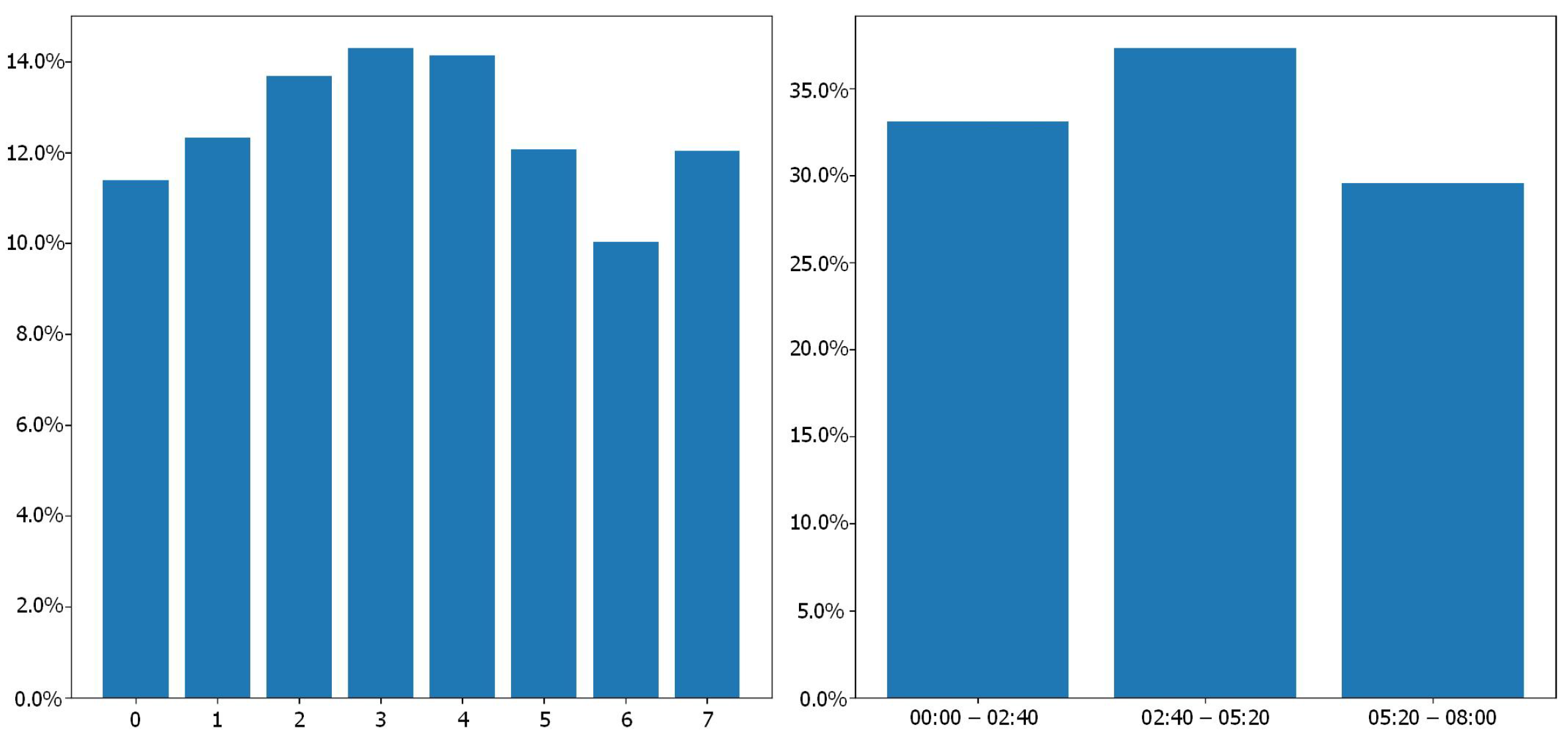
• More than 70% of the discharges were of the IC type, mainly of negative polarity. This result is in agreement with the overall ratio given in the literature, in which, although dependent on the type of storm, the latitude, and other parameters, CG discharges constitute overall 25% and IC discharges 75% of the atmospheric electrical activity (e.g., [47]);
• The highest peak currents were obtained for CG discharges, where the maximum peak corresponded to +CG discharges (322 kA), followed by −CG discharges (267 kA). Both occurred between 05:20 and 08:00 UTC (02:20 LT and 05:00 LT). In this time period, the average peak currents were 34 kA for +CG and 20 kA for −CG. These average peak current values are in agreement with the values found in [48], which, for our study area, range from 10 kA to 30 kA. Also, the estimated average peak current (34 kA) is consistent with [49], in which data were obtained using direct measurements.

3.2. Analysis of Ionospheric DVTEC Disturbances

In this section, we analyze the DVTEC disturbances generated by the storm on 10 November 2018. Subsequently, we make a comparison of the ionospheric response produced on this day, when Atmospheric Electrical Activity was present, with the ionospheric response of a day without electrical activity (9 September 2018). Finally, we analyze the data by applying the wavelet transform to the DVTEC values.

3.2.1. DVTEC Variations Due to Thunderstorms

Three geographical zones were defined for analysis purposes, as illustrated in Figure 9. In addition, the figure shows the RAMSAC stations and the lightning counts on a grid of a 0.2° by 0.2° cells. The working zones represent the following:

• Zone 1: The thunderstorms’ region;
• Zone 2: The region around the thunderstorms and adjacent to them; and
• Zone 3: The area away from the thunderstorms.

Figure 10 illustrates the variation in DVTEC on 10 November 2018 across multiple stations and GNSS satellites. This figure provides a visual representation of the DVTEC changes observed within the specified analysis zones. Results from each station are vertically offset from the previous station by 1 TECU $({10}^{16}$ electrons/m${}^2$). In each plot, the three time intervals defined in the previous section are marked with different colors in the horizontal axis in decimal time. The interval from 0 UTC to 2.66 UTC (i.e., 00:00 UTC–02:40 UTC) is marked in blue, the interval from 2.66 UTC to 5.33 UTC (i.e., 02:40 UTC–05:20 UTC) is marked in yellow, and the interval from 5.33 UTC to 8 UTC (i.e., 05:20 UTC–08:00 UTC) is marked in green. Additionally, on each graph, the names of the stations exhibiting large deviations in DVTEC, with peak-to-peak amplitudes greater than 1 TECU, are highlighted in light blue on the vertical axis. Comparing the graphs in Figure 10, it is observed that the signals became progressively more unstable, especially in Zone 3 (see in Figure 10c). Analyzing the temporal evolution of the signals within each zone, it is evident that the most significant magnitude variations occurred during the interval from 02:40 UTC to 05:20 UTC, coinciding with the peak in thunderstorm electrical activity.

The analysis performed showed that the peak-to-peak amplitudes of the DVTEC variations were different for each station and satellite. Figure 11, Figure 12 and Figure 13 present the positions of the RAMSAC stations and their respective peak-to-peak DVTEC amplitude ranges. The peak-to-peak amplitude ranges were calculated for each time interval, i.e., the peak-to-peak amplitude range corresponding to the period 00:00 UTC–02:40 UTC is presented in the upper left panel, the amplitude range for the interval 02:40 UTC–05:20 UTC in the upper right panel, and the range for 05:20 UTC–08:00 UTC in the lower left panel. The figures also include the lightning counts plotted on the 0.2° by 0.2° grid for each of the analyzed time periods. Each station is represented by a diamond, whose color indicates the peak-to-peak DVTEC range measured at that station. The locations of the events reported by the Earth Networks system to have the maximum peak currents for the different discharge types are represented by stars.

In the period 00:00 UTC–02:40 UTC (i.e., 21:00 LT–23:40 LT), a predominance of peak-to-peak DVTEC amplitudes between 0.21 TECU and 0.44 TECU was observed in all three zones. In Zones 1 and 2, peak-to-peak DVTEC amplitudes averaged 0.3 TECU, while, in Zone 3, they averaged 0.22 TECU. In this time interval, peak-to-peak DVTEC amplitude values of up to 0.67 TECU were observed. In Zone 1, the peak-to-peak DVTEC amplitude maxima surrounded the storms, while, in Zones 2 and 3, the maxima were generally located in the western region of the country. Recall that, for this time period, the storm was in its growth phase.

From 02:40 UTC–05:20 UTC (i.e., 23:40 LT–02:20 LT), a predominance of peak-to-peak DVTEC amplitudes between 0.44 TECU and 0.67 TECU was observed in all three zones. Average peak-to-peak DVTEC amplitudes of 0.61 TECU, 0.65 TECU, and 0.57 TECU were obtained for Zones 1, 2, and 3, respectively. Peak-to-peak DVTEC amplitude values of up to 1.11 TECU were observed for Zone 1 and 1.35 TECU for Zones 2 and 3. These maxima were located, for Zone 1, mainly between the storms (Figure 11), while, for Zones 2 and 3 (Figure 12 and Figure 13), they were located over the mountain range. In this time period, the storms were in their development–maturity phase.

Finally, in the time interval 05:20 UTC–08:00 UTC (02:20 LT–05:00 LT), peak-to-peak DVTEC amplitude values of up to 0.67 TECU were observed, mainly located in the northern region of the country. Likewise, a predominant peak-to-peak DVTEC amplitude between 0.21 TECU and 0.44 TECU was observed. An average peak-to-peak DVTEC amplitude of 0.25 TECU for Zones 1 and 3 and of 0.3 TECU for Zone 2 were also observed. During this time period, thunderstorm electrical activity was decreasing.

3.2.2. Comparison with a Day without Storms

To analyze the ionospheric behavior during a thunderstorm, we chose a day in Argentina with no atmospheric electrical activity (AEA). We designated 9 September 2018 as the base day for comparative purposes. In this study, we chose 14 RAMSAC stations, whose distribution can be seen in Figure 14. The right image in the figure represents the lightning counts on a 0.2° by 0.2° grid. The points where the peak current of the different types of discharges were reported to have occurred by the Earth Network system are marked with a star. From Figure 14, we observe that the RAMSAC stations are distributed as follows:

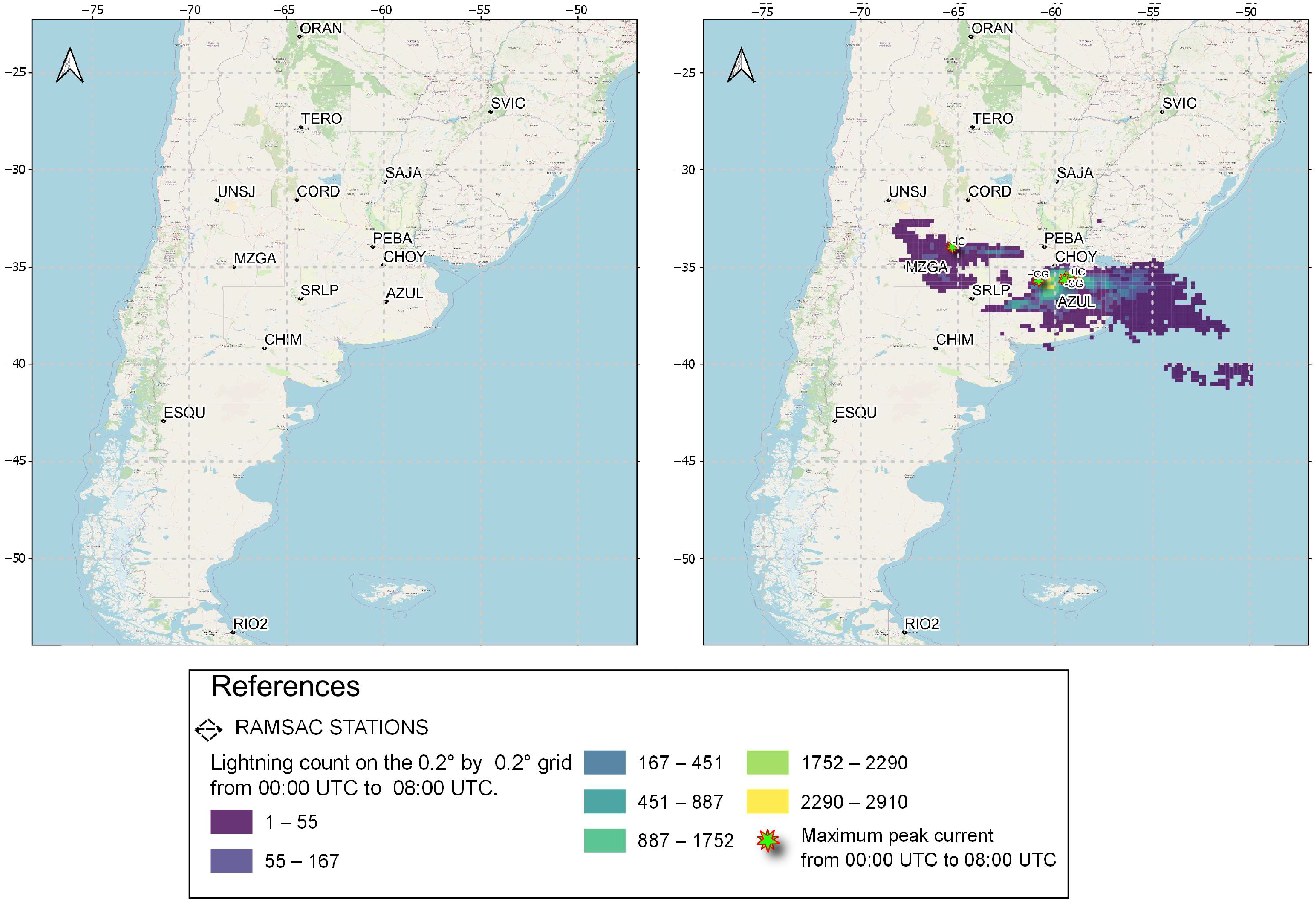
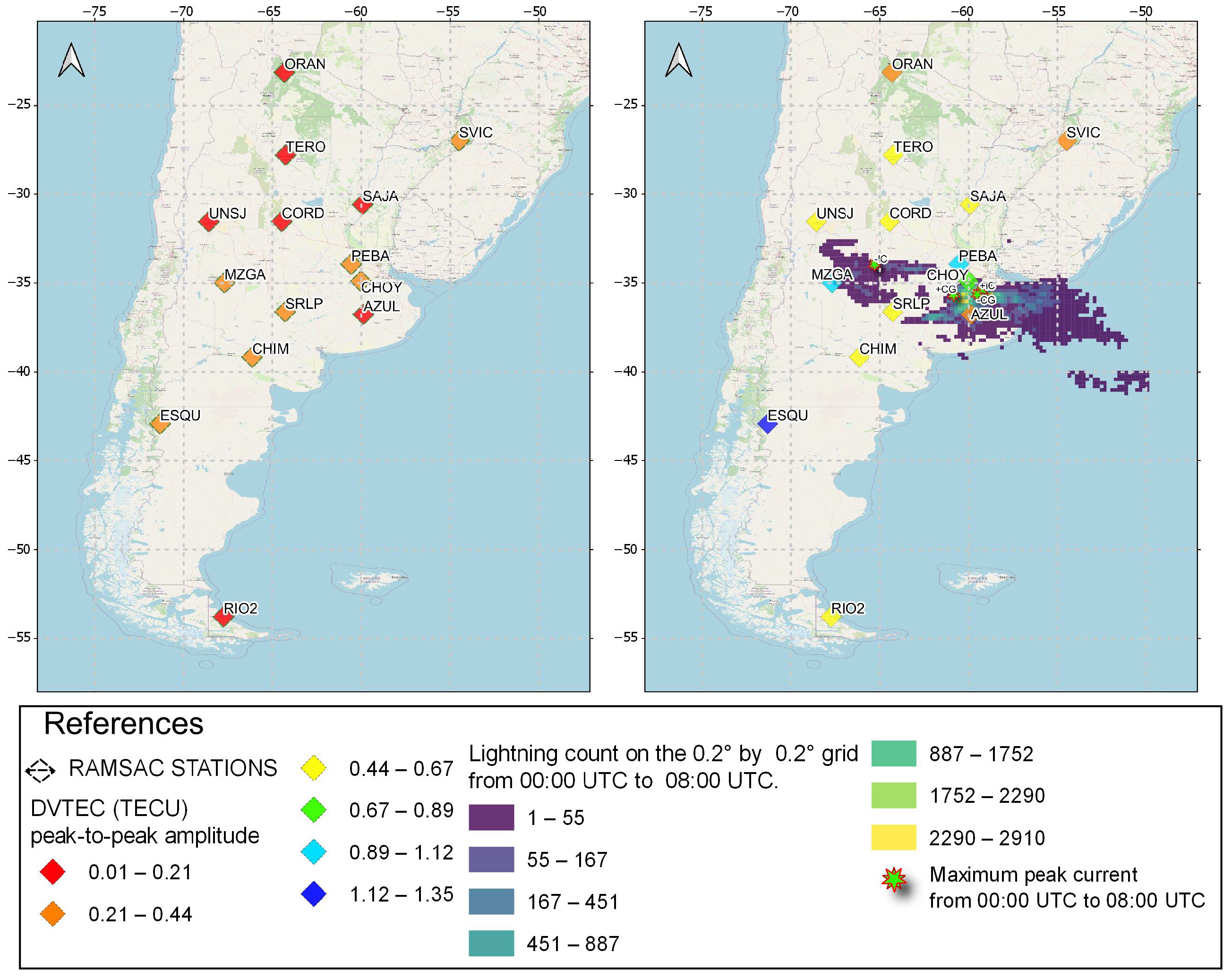
• Six stations in Zone 1: AZUL, CHOY, CORD, MZGA, PEBA, SRLP;
• Three stations in Zone 2: CHIM, SAJA, UNSJ; and
• Five stations in Zone 3: ESQU, ORAN, RIO2, SVIC, TERO.

In addition, we can see that the AZUL and CHOY stations were the closest to the regions with the highest number of discharges. These stations, together with MZGA, were located near the highest current peaks. Note that SRLP and PEBA were located between the storms.

When comparing the DVTEC variations between the two days (refer to Figure 15), it is evident that the day with AEA exhibited significant fluctuations in DVTEC. The stations with the highest variability are highlighted in light blue in Figure 15b. Three of the stations, namely, CHOY, MZGA, and PEBA, are situated in Zone 1, which corresponded to the storm region. Furthermore, the ESQU station also recorded considerable deviations in DVTEC, despite being located in Zone 3, specifically, in the Andes mountain range.

The peak-to-peak DVTEC amplitudes for each station throughout the study period (00:00 UTC–08:00 UTC) are shown in Figure 16 using multicolored diamonds, representing both the reference day (left panel) and the day with AEA (right panel). The lightning counts are also plotted on 0.2° by 0.2° grid. The points where the maximum peak current of the different types of discharges occurred are marked with stars. On the reference day, the peak-to-peak DVTEC amplitudes measurements from all the stations collectively spanned from 0.01 to 0.44 TECU. Conversely, on the day with AEA, peak-to-peak DVTEC amplitudes ranged from 0.21 TECU to 1.35 TECU. This indicates an increase in amplitude across all stations, likely due to the presence of thunderstorms. It is worth noting that, although stations CHOY and AZUL were located near the area of maximum discharge and peak current, they exhibited differences in their amplitude values. The same occurred with PEBA and SRLP, which were situated between the storms. Note that peak-to-peak DVTEC amplitudes ranging from 0.44 TECU to 0.67 TECU are predominant in the data.

Table 3. Peak-to-peak DVTEC amplitude of the 14 RAMSAC stations, for the reference and storm day in the whole study period (00:00 UTC–08:00 UTC). Table created by author.

	Peak-to-Peak DVTEC Amplitude (TECU)
RAMSAC Stations	Day without AEA (Reference Day)	Day with AEA
AZUL	0.16	0.32
CHIM	0.27	0.66
CHOY	0.31	0.87
CORD	0.20	0.53
ESQU	0.32	1.35
MZGA	0.26	0.93
ORAN	0.19	0.37
PEBA	0.29	0.91
RIO2	0.18	0.63
SAJA	0.20	0.65
SRLP	0.23	0.53
SVIC	0.25	0.40
TERO	0.21	0.64
UNSJ	0.21	0.55

shows the DVTEC peak-to-peak amplitude of the 14 analyzed stations for the entire study period (00:00 UTC–08:00 UTC). In the table we can see that stations ESQU, MZGA, PEBA, RIO2, SAJA and TERO experienced an increase in their DVTEC peak-to-peak amplitudes of three or more times during the day of the storm compared to their reference peak-to-peak amplitude values. ESQU and RIO2 were situated south of the storm region and MZGA was within the storm zone, while PEBA, SAJA, and TERO were located north of the storm region.

By calculating the average peak-to-peak DVTEC amplitude of the 14 stations for the reference day, we obtained an average peak-to-peak amplitude of 0.23 TECU. On the other hand, the average peak-to-peak amplitude for the AEA day was 0.67 TECU. Comparing both results, we can see that, on a stormy day, the average peak-to-peak amplitude increased by a factor of 2.91 with respect to the average peak-to-peak amplitude of the non-stormy day.

3.2.3. DVTEC Signal Period Analysis

In order to analyze the periods present in the DVTEC signal and its amplitude spectrum, the C-Morlet 1.5 wavelet transform was applied to five RAMSAC stations strategically selected in relation to the storm cells. Figure 17 shows the chosen stations (AZUL, MZGA, PEBA, SRLP, and TERO), along with the DVTEC measurement paths of each satellite and the DVTEC peak-to-peak amplitudes during the entire study period (00:00 UTC–08:00 UTC). In the map on the right, lightning is plotted on a 0.2° by 0.2° grid, and the locations where the maximum current peaks were recorded are indicated by stars. Observing the map on the right, we can notice that stations MZGA, PEBA, and TERO present a predominantly longitudinal path of their satellites, while stations AZUL and SRLP show a mostly latitudinal path, especially after 03:00 UTC.

Continuing with the analysis, we examine the DVTEC variation for the selected five stations on the days both without and with AEA (refer to Figure 18). For the day without AEA, we observed DVTEC fluctuations with high frequency (Figure 18a) and peak-to-peak DVTEC amplitudes ranging from 0.16 TECU to 0.29 TECU (see Table 3). On the other hand, for the day with AEA, we found DVTEC fluctuations with both low and high frequencies (Figure 18b) and higher peak-to-peak amplitudes ranging from 0.32 TECU to 0.93 TECU (Table 3). In addition, during the day with AEA, we observe that the stations tended to reach their maximum DVTEC variation between 03:00 UTC and 05:00 UTC. After that time, they tended to return to their nominal state.

We applied the wavelet transform to the data both for the day with the storm and for the day without the storm. Figure 19, Figure 20, Figure 21, Figure 22 and Figure 23 show, for each station and GNSS satellite, the satellite path in decimal time (UTC), the peak-to-peak DVTEC amplitude (TECU), the lightning counts on the 0.2° by 0.2° grid, and the position of the maximum current peaks. In the lower-left panel, we show the DVTEC variation of the processed satellite data in decimal hours for both days. To the right of that panel, we show the continuous wavelet transform calculation with its confidence cone, which represents the 95% confidence for the result obtained within it. By observing the maps along with the temporal variation graphs of DVTEC (bottom left panel), we find the highest DVTEC variations as follows:

• The AZUL station satellite (Figure 19) passes through the southeast storm. The maximum peak of variation is reached between about 03:50 UTC and 05:00 UTC, when it is passing through the area with the highest number of discharges;
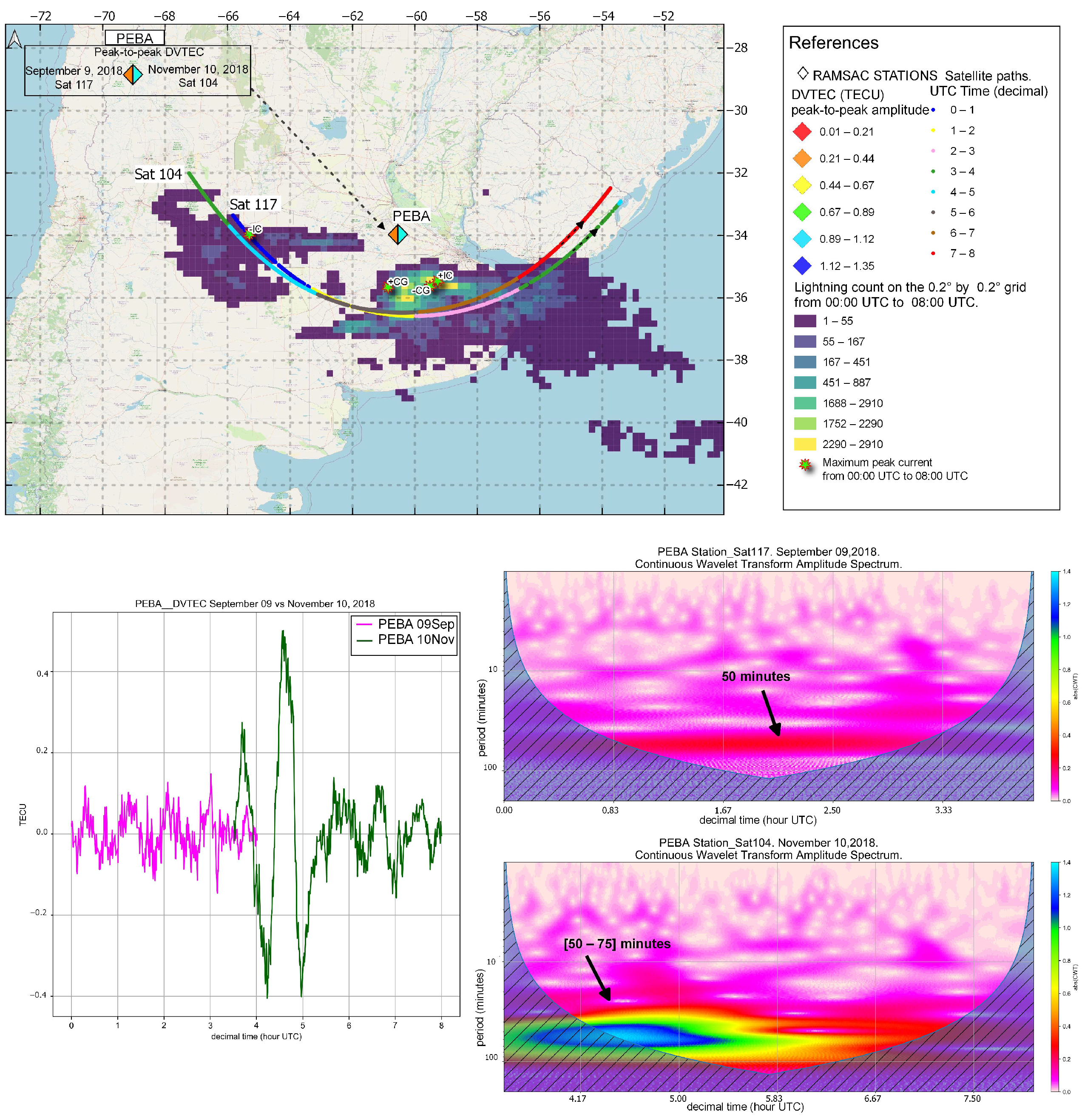
• The satellite of the PEBA station (Figure 21) crosses the storm located in the central region. This occurs between 04:00 UTC and 05:00 UTC;
• The satellites of stations MZGA (Figure 20) and TERO (Figure 23) cross the area in the Andes Mountains. The maximum variations of MZGA and TERO occur between 03:00 UTC and 04:00 UTC and between 04:00 UTC and 05:00 UTC, respectively;
• The satellite of the SRLP station (Figure 22) crosses the Andes Mountains. In addition, we found the largest DVTEC variations when the satellite passed through the storm region. The first maximum occurs between 01:00 UTC and 02:00 UTC, and the second between 03:00 UTC and 04:00 UTC.

In these cases, we do not detect an at-a-glance relationship between the maximum peak currents and the maximum variations in the DVTEC of each station, since they occur at different times and locations.

Finally, as mentioned previously, Figure 19, Figure 20, Figure 21, Figure 22 and Figure 23 present the wavelet transform of the five studied stations. Observing these figures, we see that, for the day without AEA, the period of the DVTEC signal was less than 75 min, the peak-to-peak DVTEC amplitude was between 0.16 and 0.29 TECU and the spectral amplitude was between 0.1 and 0.2. On the other hand, for the day with AEA, we find periods lower than 100 min, peak-to-peak DVTEC amplitudes between 0.32 and 0.93 TECU, and spectral amplitudes between 0.25 and 1.4.

4. Discussion

Between 00:00 UTC and 08:00 UTC on 10 November 2018, two storms moved southeastward in Argentina. While the storm situated in the central region of the country was in the developmental stage, the other storm, located in the southeast region of the country, had already reached the maturity stage. The difference in their life stages led to the observation of a greater number of discharges in the southeastern storm compared to the central storm, where lightning was found mainly at temperatures lower than −70 °C, i.e., in the deep convective zones.

Based on the research conducted by [3,5] regarding the variation and ionospheric effects in gravity waves in Total Electron Content (TEC) records during storms in mid- and low-latitude areas, respectively, our analysis was divided into three periods to highlight the variability in the waves generated by the storms. Through this analysis, we found the following:

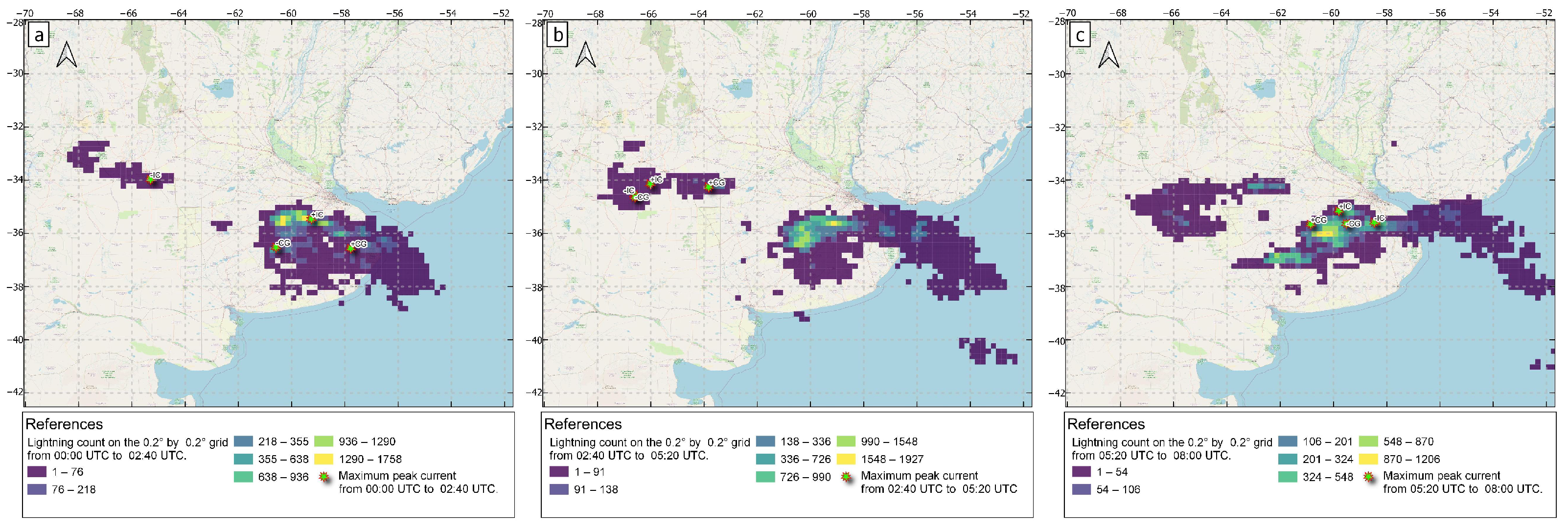
• In the period between 00:00 UTC and 02:40 UTC (21:00 LT–23:40 LT), the RAMSAC stations showed DVTEC oscillations with peak-to-peak amplitude values of up to 0.67 TECU. Earth Networks lightning detection system reported peak current maxima of −219 kA for −CG and 181 kA for +CG. These maxima were located over the southeast of the storm, near the regions with the highest lightning count. In proximity to these regions, the AGGO, AZUL, CHOY, LPGS, and PEBA stations showed peak-to-peak DVTEC amplitudes of up to 0.44 TECU. During this period, the storms were in their growth stage;
• Between 02:40 UTC and 05:20 UTC (23:40 LT–02:20 LT), RAMSAC stations showed oscillations in the DVTEC with peak-to-peak amplitude values of up to 1.35 TECU. The maximum peak currents were −214 kA for −CG and 211 kA for +CG, located above the storm located in the central region. In proximity to the areas with the highest lightning frequency and peak current, the AGGO, AZUL, CHOY, GVIL, MZAE, MZAU, MZGA, NUGA, RIO4, RUFI, and PEJO stations showed peak-to-peak DVTEC amplitudes of up to 1.12 TECU. During this period, the storms were in their development phase. In addition, during this time, the highest number of lightning flashes occurred and the highest peak-to-peak amplitudes were observed in the three analyzed zones;
• In the period between 05:20 and 08:00 UTC (02:20 LT–05:00 LT), RAMSAC stations showed DVTEC oscillations with peak-to-peak amplitude values of up to 0.67 TECU. In the southern region of Zone 3 (see Figure 13), the perturbations found could not be directly attributed to the storms analyzed, since they were located in a region where a large number of gravity waves were produced [50]. Moreover, current peaks in +CG of 322 kA and −CG of −267 kA were observed in this period. These peaks were located near the regions with the highest number of lightning flashes over the storm to the southeast. During this period, the storms showed a decrease in their atmospheric electrical activity.

Across the various time segments, we identified waveform structures in DVTEC, with peak-to-peak amplitudes ranging from 0.01 to 1.35 TECU. Notably, we were able to observe, within the time window [02:40–05:20] UTC, corresponding to the period in which the highest lightning count occurred, the highest peak-to-peak DVTEC amplitudes.

Then, we worked with a base day (reference day), in which the geomagnetic activity was low and the electrical activity was null for the whole study period in Argentina. At this point, we worked only with 14 RAMSAC stations. Comparing the peak-to-peak DVTEC amplitude of the reference value with the peak-to-peak DVTEC amplitude of the day with AEA for the whole study period (00:00 UTC–08:00 UTC), it was observed that the 14 stations presented variations during the stormy day.

From Table 3, we observe that wave amplitudes experienced a 2.91-fold increase compared to the day without AEA. When examining the ESQU station, it is evident that it exhibited the highest peak-to-peak amplitude and was located significantly distantly from the storm region. In contrast, the AZUL and CHOY stations, situated over the storm area and specifically within the region of higher electrical activity, displayed lower amplitudes. This finding contrasts with expectations, as one would anticipate greater variations in the storm region (Zone 1). These discrepancies are clearly visible in Figure 10, where it can be seen that, as we move away from the storm area, the variability in the waves increases. These variations could be attributed to gravity and medium-scale wave propagation processes, as detailed in the introduction. The alignment and direction of the medium-scale waves (NE–SW) could explain the differences observed in Figure 16 between the day without a storm and the day with the storm, where these differences are accentuated.

Therefore, we infer that the storms could have generated gravity waves and that the remarkable differences found could be due to the interaction of these waves with another source of gravity waves. In this context, the Andes Mountains, the Antarctic Peninsula, and the Patagonian region have the potential to generate such waves. These areas are considered the epicenter of the most intense gravity wave activity worldwide, as highlighted in the studies in [51,52].

Finally, five stations close to the region where the storms developed were analyzed for both days. From the wavelet analysis, variabilities with periods less than or equal to 100 min, spectral amplitudes up to 1.4, and peak-to-peak DVTEC amplitudes up to 0.93 TECU were obtained during the day with the storm. Conversely, during the reference day, wavelets with periods less than 75 min, spectral amplitudes up to 0.2, and peak-to-peak DVTEC amplitudes up to 0.29 TECU were observed.

5. Conclusions

To sum up, we performed an electrical characterization of the thunderstorms that took place in central Argentina on 10 November 2018 and observed their effect on the ionosphere. As a result, we obtained that the thunderstorm produced disturbances with periods less than or equal to 100 min and peak-to-peak DVTEC amplitudes up to 1.35 TECU. These findings are in agreement with the investigations of [44,53], which identified waves with similar periodicities and determined average periods for different regions of the world. These disturbances, known as atmospheric gravity waves, appeared to be related to the thunderstorms. Indeed, when the highest lightning count occurred, the highest peak-to-peak amplitudes were obtained in the DVTEC. Therefore, the observed increase in amplitude could be related to an intensification of the updraft or to some other microphysical parameters of the thunderstorm.

Another study [1] established a direct relationship between increased thunderstorm activity and DVTEC amplitudes. They found that average disturbance amplitudes on days with severe thunderstorms were 1.3 times higher than on those without thunderstorms. In our case, the average peak-to-peak amplitude on the day with thunderstorms was approximately 2.91 times higher than on the day without. These findings highlight the significant influence of storms on ionospheric variations and underscore the importance of understanding how different factors can contribute to these observed perturbations in the ionosphere.

Considering that CG discharges constitute 25% and IC discharges 75% of the atmospheric electrical activity [47], we can conclude that the results found in the percentage of discharges was as expected, since more than 70% of the discharges were of the IC type, mainly of negative polarity. Although we obtained this proportion, we have not yet been able to determine which type of lightning activity plays a fundamental role in the generation of gravity waves in the atmosphere.

When comparing the analyzed DVTEC signals, a progressive increase in instability was observed as we moved away from the storm zone. According to [54], “This may occur since, under suitable conditions, gravity waves as they propagate upward become unstable at higher altitudes and may break up (at an altitude of about 100 km) into secondary waves [12] which continue to propagate upward, possibly modulating the E-region plasma distribution producing polarization electric fields that map the F-region ionosphere [55].” Moreover, there are authors, such as [56,57], who suggest that these disturbances in the ionosphere may be due to vertical transport of electrostatic discharge [4]. Others have suggested [58] that this may be caused by Transient Luminous Events (TLEs), which would induce fluctuations in the D region of the ionosphere [4]. This would indicate that gravity waves can be found beyond the thunderstorm zone.

In the investigation of gravity waves generated in our territory, it is essential to consider not only the regional seismic activity, the presence of storms, and weather fronts, but also the influence of the Andes Mountains and the local effect of Patagonia, as they have recently been identified as the epicenter of the most intense gravity wave activity in the world [51,52]. These elements could potentially converge to generate a coupling phenomenon in gravity waves originating in the region. Additionally, we should consider medium-scale traveling disturbances since, for mid-latitudes, they exhibit a specific alignment and direction in each hemisphere [14]. Consequently, decoupling these wave phenomena is a challenge, since they could also contribute to the studied aspects; we intend to study these due to the unique characteristics of the investigated region.

References

1. Rahmani, Y.; Alizadeh, M.M.; Schuh, H.; Wickert, J.; Tsai, L.C. Probing vertical coupling effects of thunderstorms on lower ionosphere using GNSS data. Adv. Space Res. 2020, 66, 1967–1976. [Google Scholar] [CrossRef]
2. Chapman, S. The atmospheric height distribution of band-absorbed solar radiation. Proc. Phys. Soc. 1939, 51, 93. [Google Scholar] [CrossRef]
3. Lay, E.H.; Shao, X.M.; Kendrick, A.K.; Carrano, C.S. Ionospheric acoustic and gravity waves associated with midlatitude thunderstorms. J. Geophys. Res. Space Phys. 2015, 120, 6010–6020. [Google Scholar] [CrossRef]
4. Ogunsua, B.; Srivastava, A.; Bian, J.; Qie, X.; Wang, D.; Jiang, R.; Yang, J. Significant day-time ionospheric perturbation by thunderstorms along the West African and Congo sector of equatorial region. Sci. Rep. 2020, 10, 8466. [Google Scholar] [CrossRef] [PubMed]
5. Lay, E.H.; Shao, X.M.; Carrano, C.S. Variation in total electron content above large thunderstorms. Geophys. Res. Lett. 2013, 40, 1945–1949. [Google Scholar] [CrossRef]
6. Liu, T.; Yu, Z.; Ding, Z.; Nie, W.; Xu, G. Observation of Ionospheric Gravity Waves Introduced by Thunderstorms in Low Latitudes China by GNSS. Remote Sens. 2021, 13, 4131. [Google Scholar] [CrossRef]
7. Cheng, Z.; Cummer, S.A. Broadband VLF measurements of lightning-induced ionospheric perturbations. Geophys. Res. Lett. 2005, 32, 8. [Google Scholar] [CrossRef]
8. Vadas, S.; Liu, H.L. Numerical modeling of the large-scale neutral and plasma responses to the body forces created by the dissipation of gravity waves from 6 h of deep convection in Brazil. J. Geophys. Res. Space Phys. 2013, 118, 2593–2617. [Google Scholar] [CrossRef]
9. Vadas, S.L.; Fritts, D.C. Thermospheric responses to gravity waves arising from mesoscale convective complexes. J. Atmos. Sol.-Terr. Phys. 2004, 66, 781–804. [Google Scholar] [CrossRef]
10. Walterscheid, R.; Schubert, G.; Brinkman, D. Acoustic waves in the upper mesosphere and lower thermosphere generated by deep tropical convection. J. Geophys. Res. Space Phys. 2003, 108, A11. [Google Scholar] [CrossRef]
11. Zettergren, M.; Snively, J. Ionospheric signatures of acoustic waves generated by transient tropospheric forcing. Geophys. Res. Lett. 2013, 40, 5345–5349. [Google Scholar] [CrossRef]
12. Snively, J.B.; Pasko, V.P. Breaking of thunderstorm-generated gravity waves as a source of short-period ducted waves at mesopause altitudes. Geophys. Res. Lett. 2003, 30, 24. [Google Scholar] [CrossRef]
13. Vadas, S.L.; Liu, H.l. Generation of large-scale gravity waves and neutral winds in the thermosphere from the dissipation of convectively generated gravity waves. J. Geophys. Res. Space Phys. 2009, 114, A10. [Google Scholar] [CrossRef]
14. Heale, C.; Inchin, P.; Snively, J. Primary Versus Secondary Gravity Wave Responses at F-Region Heights Generated by a Convective Source. J. Geophys. Res. Space Phys. 2022, 127, e2021JA029947. [Google Scholar] [CrossRef]
15. Asiares, C.I.V.; Nicora, M.G.; Meza, A.; Paula, M.; Avila, E.E. Relationship between the activity of thunderstorms and ionospheric oscillation during the RELAMPAGO Project. In Proceedings of the 2021 35th International Conference on Lightning Protection (ICLP) and XVI International Symposium on Lightning Protection (SIPDA), Colombo, Sri Lanka, 20–26 September 2021; Volume 1, pp. 1–7. [Google Scholar]
16. Zipser, E.J.; Cecil, D.J.; Liu, C.; Nesbitt, S.W.; Yorty, D.P. Where are the most intense thunderstorms on Earth? Bull. Am. Meteorol. Soc. 2006, 87, 1057–1072. [Google Scholar] [CrossRef]
17. Cecil, D.J.; Blankenship, C.B. Toward a global climatology of severe hailstorms as estimated by satellite passive microwave imagers. J. Clim. 2012, 25, 687–703. [Google Scholar] [CrossRef]
18. Piscitelli, F.M.; Ruiz, J.J.; Negri, P.; Salio, P. A multiyear radar-based climatology of supercell thunderstorms in central-eastern Argentina. Atmos. Res. 2022, 277, 106283. [Google Scholar] [CrossRef]
19. Corrales, P.B.; Galligani, V.; Ruiz, J.; Sapucci, L.; Dillon, M.E.; Skabar, Y.G.; Sacco, M.; Schwartz, C.S.; Nesbitt, S.W. Hourly assimilation of different sources of observations including satellite radiances in a mesoscale convective system case during RELAMPAGO campaign. Atmos. Res. 2022, 281, 106456. [Google Scholar] [CrossRef]
20. Bechis, H.; Galligani, V.; Imaz, M.A.; Cancelada, M.; Simone, I.; Piscitelli, F.; Maldonado, P.; Salio, P.; Nesbitt, S.W. A case study of a severe hailstorm in Mendoza, Argentina, during the RELAMPAGO-CACTI field campaign. Atmos. Res. 2022, 271, 106127. [Google Scholar] [CrossRef]
21. Kumjian, M.R.; Gutierrez, R.; Soderholm, J.S.; Nesbitt, S.W.; Maldonado, P.; Luna, L.M.; Marquis, J.; Bowley, K.A.; Imaz, M.A.; Salio, P. Gargantuan hail in Argentina. Bull. Am. Meteorol. Soc. 2020, 101, E1241–E1258. [Google Scholar] [CrossRef]
22. Arena, L.E. Granizos Gigantes de Córdoba-Argentina I. El Coloso Victoria, 2000. Repositorio Digital, Universidad Nacional de Córdoba. Available online: http://hdl.handle.net/11086/15963 (accessed on 26 August 2023).
23. Nesbitt, S.W.; Salio, P.V.; Ávila, E.; Bitzer, P.; Carey, L.; Chandrasekar, V.; Deierling, W.; Dominguez, F.; Dillon, M.E.; Garcia, C.M.; et al. A storm safari in subtropical South America: Proyecto RELAMPAGO. Bull. Am. Meteorol. Soc. 2021, 102, E1621–E1644. [Google Scholar] [CrossRef]
24. Varble, A.C.; Nesbitt, S.W.; Salio, P.; Hardin, J.C.; Bharadwaj, N.; Borque, P.; DeMott, P.J.; Feng, Z.; Hill, T.C.; Marquis, J.N.; et al. Utilizing a storm-generating hotspot to study convective cloud transitions: The CACTI experiment. Bull. Am. Meteorol. Soc. 2021, 102, E1597–E1620. [Google Scholar] [CrossRef]
25. National Science Foundation. RELAMPAGO-CACTI Campaign. 2018. Available online: https://catalog.eol.ucar.edu/relampago (accessed on 26 August 2023).
26. SpaceWeatherLive is an initiative of Parsec vzw, a.B.n.p.o. “SpaceWeatherLive.Com | Real-Time Data and Plots Auroral Activity” n.d. 2008. Available online: https://www.spaceweatherlive.com/ (accessed on 26 August 2023).
27. Networks, E. Earth Networks Total Lightning Network. Available online: https://www.earthnetworks.com/why-us/networks/lightning/ (accessed on 26 August 2023).
28. Zhu, Y.; Stock, M.; Lapierre, J.; DiGangi, E. Upgrades of the Earth networks total lightning network in 2021. Remote Sens. 2022, 14, 2209. [Google Scholar] [CrossRef]
29. Networks, E. Earth Networks Total Lightning Network (ENTLN) Global Lightning Network. Available online: https://ghrc.nsstc.nasa.gov/home/content/earth-networks-total-lightning-network-entln-global-lightning-network (accessed on 26 August 2023).
30. This Page Is Maintained by University of Utah © 2020, Department of Atmospheric Science, U.o.U. GOES-16/17/18 on Amazon Download Page. 2020. Available online: https://home.chpc.utah.edu/~u0553130/Brian_Blaylock/cgi-bin/goes16_download.cgi?source=aws&satellite=noaa-goes16&domain=F&product=ABI-L2-MCMIP&date=2018-12-14&hour=9 (accessed on 26 August 2023).
31. Schmit, T.J.; Griffith, P.; Gunshor, M.M.; Daniels, J.M.; Goodman, S.J.; Lebair, W.J. A closer look at the ABI on the GOES-R series. Bull. Am. Meteorol. Soc. 2017, 98, 681–698. [Google Scholar] [CrossRef]
32. Berrick, N.O.S. Crustal Dynamics Data Information System. Available online: https://urs.earthdata.nasa.gov/oauth/authorize?client_id=gDQnv1IO0j9O2xXdwS8KMQ&response_type=code&redirect_uri=https%3A%2F%2Fcddis.nasa.gov%2Fproxyauth&state=aHR0cDovL2NkZGlzLm5hc2EuZ292L2FyY2hpdmUvZ25zcy8 (accessed on 26 August 2023).
33. IGN. Instituto Geográfico Nacional. Available online: https://www.ign.gob.ar/ (accessed on 26 August 2023).
34. Adler, R.F.; Mack, R.A. Thunderstorm cloud top dynamics as inferred from satellite observations and a cloud top parcel model. J. Atmos. Sci. 1986, 43, 1945–1960. [Google Scholar] [CrossRef]
35. Borque, P.; Vidal, L.; Rugna, M.; Lang, T.J.; Nicora, M.G.; Nesbitt, S.W. Distinctive signals in 1-min observations of overshooting tops and lightning activity in a severe supercell thunderstorm. J. Geophys. Res. Atmos. 2020, 125, e2020JD032856. [Google Scholar] [CrossRef]
36. Chris Vagasky, V.X.; Total Lightning Statistics 2022. The Annual Lightning Report. 2022, p. 8. Available online: https://indd.adobe.com/view/d0591066-471e-41b9-83e1-4dc937aaeb96 (accessed on 26 August 2023).
37. Dach, R.; Lutz, S.; Walser, P.; Fridez, P. Bernese GNSS Software Version 5.2; Astronomical Institute, University of Bern: Bern, Switzerland, 2015. [Google Scholar]
38. Petit, G.; Luzum, B. The 2010 reference edition of the IERS conventions. In Reference Frames for Applications in Geosciences; Springer: Berlin, Germany, 2013; pp. 57–61. [Google Scholar]
39. Letellier, T. Etude Des Ondes de Marée sur les Plateaux Continentaux. Ph.D. Thesis, Toulouse 3, Toulouse, France, 2005. [Google Scholar]
40. van Dam, T.; Altamimi, Z.; Collilieux, X.; Ray, J. Topographically induced height errors in predicted atmospheric loading effects. J. Geophys. Res. Solid Earth 2010, 115, B7. [Google Scholar] [CrossRef]
41. MAGGIA-FCAG-UNLP. MAGGIA Laboratory. Available online: https://www.maggia.unlp.edu.ar/ (accessed on 26 August 2023).
42. Meza, A.; Van Zele, M.A.; Rovira, M. Solar flare effect on the geomagnetic field and ionosphere. J. Atmos. Sol. Terr. Phys. 2009, 71, 1322–1332. [Google Scholar] [CrossRef]
43. Meza, A.; Bosch, G.; Natali, M.P.; Eylenstein, B. Ionospheric and geomagnetic response to the total solar eclipse on 21 August 2017. Adv. Space Res. 2022, 69, 16–25. [Google Scholar] [CrossRef]
44. Chowdhury, S.; Kundu, S.; Ghosh, S.; Sasmal, S.; Brundell, J.; Chakrabarti, S.K. Statistical study of global lightning activity and thunderstorm-induced gravity waves in the ionosphere using WWLLN and GNSS-TEC. J. Geophys. Res. Space Phys. 2023, 128, e2022JA030516. [Google Scholar] [CrossRef]
45. Burrell, A.G.; Bonito, N.A.; Carrano, C.S. Total electron content processing from GPS observations to facilitate ionospheric modeling. GPS Solut. 2009, 13, 83–95. [Google Scholar] [CrossRef]
46. Fernández-Lavín, A.; Ovando-Shelley, E. Interpretación de señales usando transformadas wavelet continuas. In Proceedings of the Geotechnical Engineering in the XXI Century: Lessons Learned and Future Challenges: Proceedings of the XVI Pan-American Conference on Soil Mechanics and Geotechnical Engineering (XVI PCSMGE), Cancun, México, 17–20 November 2019; p. 138.
47. Nicora, M.G. Actividad eléctrica atmosférica en Sudamérica. Ph.D. Thesis, Universidad Nacional de La Plata, Provincia de Buenos Aires, Argentina, 2014. [Google Scholar]
48. DiGangi, E.; Lapierre, J.; Stock, M.; Hoekzema, M.; Cunha, B. Analyzing lightning characteristics in central and southern South America. Electr. Power Syst. Res. 2022, 213, 108704. [Google Scholar] [CrossRef]
49. Berger, K. Parameters of lightning flashes. Electra 1975, 80, 223–237. [Google Scholar]
50. Wu, D.L.; Eckermann, S.D. Global gravity wave variances from Aura MLS: Characteristics and interpretation. J. Atmos. Sci. 2008, 65, 3695–3718. [Google Scholar] [CrossRef]
51. Alexander, P.; Luna, D.; Llamedo, P.; de la Torre, A. A gravity waves study close to the Andes mountains in Patagonia and Antarctica with GPS radio occultation observations. Ann. Geophys. 2010, 28, 587–595. [Google Scholar] [CrossRef]
52. Suzuki, S.; Nakamura, T.; Ejiri, M.K.; Tsuno, K.; Nishiyama, T.; Mizuno, A.; Salvador, J. Near-infrared camera observations of mesospheric gravity waves in Patagonia. In Proceedings of the 42nd COSPAR Scientific Assembly, Pasadena, CA, USA, 14–22 July 2018; Volume 42, p. C2-2. [Google Scholar]
53. Blanc, E.; Farges, T.; Le Pichon, A.; Heinrich, P. Ten year observations of gravity waves from thunderstorms in western Africa. J. Geophys. Res. Atmos. 2014, 119, 6409–6418. [Google Scholar] [CrossRef]
54. Kumar, S.; Chen, W.; Chen, M.; Liu, Z.; Singh, R. Thunderstorm-/lightning-induced ionospheric perturbation: An observation from equatorial and low-latitude stations around Hong Kong. J. Geophys. Res. Space Phys. 2017, 122, 9032–9044. [Google Scholar] [CrossRef]
55. Takahashi, H.; Taylor, M.J.; Pautet, P.D.; Medeiros, A.; Gobbi, D.; Wrasse, C.; Fechine, J.; Abdu, M.; Batista, I.; Paula, E.; et al. Simultaneous observation of ionospheric plasma bubbles and mesospheric gravity waves during the SpreadFEx Campaign. In Annales Geophysicae; Copernicus GmbH: Göttingen, Germany, 2009; Volume 27, pp. 1477–1487. [Google Scholar]
56. Davis, C.J.; Johnson, C.G. Lightning-induced intensification of the ionospheric sporadic E layer. Nature 2005, 435, 799–801. [Google Scholar] [CrossRef]
57. Lay, E.; Shao, X.M. Multi-station probing of thunderstorm-generated D-layer fluctuations by using time-domain lightning waveforms. Geophys. Res. Lett. 2011, 38, 23. [Google Scholar] [CrossRef]
58. Qin, J.; Pasko, V.P.; McHarg, M.G.; Stenbaek-Nielsen, H.C. Plasma irregularities in the D-region ionosphere in association with sprite streamer initiation. Nat. Commun. 2014, 5, 1–6. [Google Scholar] [CrossRef]
Figure 1. Study region outlined in orange.
Atmosphere 14 01386 g001
Figure 2. RAMSAC stations [33].
Atmosphere 14 01386 g002
Figure 3. GOES-R 16 image, channel 13 (10.3 μ m). Plots are made every two hours from 18:00 UTC on 9 November 2018 to 16:00 UTC on 10 November 2018. The study subregion, defined between latitudes 43° S–28° S and longitudes 70° W–51° W, is outlined in yellow.
Atmosphere 14 01386 g003
Figure 4. Evolution of hourly storms from 00:00 UTC to 03:00 UTC in the study subregion. Diamonds are used to represent IntraCloud (IC) discharges (brown for −IC and green for +IC), and stars to represent Cloud-to-Ground (CG) discharges (blue for −CG and light blue for +CG). The color scale represents the brightness temperature corresponding to band 13 of the ABI sensor, GOES-R 16.
Atmosphere 14 01386 g004
Figure 5. Same as Figure 4 for storms from 04:00 UTC to 07:00 UTC.
Atmosphere 14 01386 g005
Figure 6. Lightning count on the 0.2° by 0.2° grid from 00:00 to 08:00 UTC (21:00 LT–05:00 LT). Light colors represent the location with the highest lightning count. The stars indicate the sites where the maximum peak currents of the +CG, −CG, +IC, and −IC discharges occurred.
Atmosphere 14 01386 g006
Figure 7. (Left) Relative frequency of lightning at UTC hour. (Right) Relative frequency of lightning at the period of time.
Atmosphere 14 01386 g007
Figure 8. Lightning count on the 0.2° by 0.2° grid from (a) 00:00 UTC to 02:40 UTC (21:00 LT–23:40 LT), (b) 02:40 UTC to 05:20 UTC (23:40 LT–02:20 LT), and (c) 05:20 UTC to 08:00 UTC (02:20 LT–05:00 LT). Light colors represent the location with the highest lightning count. Stars indicate the locations where the peak currents of the +CG, −CG, +IC, and −IC discharges occurred.
Atmosphere 14 01386 g008
Figure 9. Lightning counts on the 0.2° by 0.2° grid from 00:00 UTC to 08:00 UTC (21:00 LT–05:00 LT). Light colors represent locations with the highest lightning counts. RAMSAC stations are marked with diamonds, and the three study zones are delimited with ellipses.
Atmosphere 14 01386 g009
Figure 10. Temporal variations in the differential vertical total electron content (DVTEC) of the RAMSAC stations within (a) Zone 1, (b) Zone 2, and (c) Zone 3. On the x-axis, with colored bars, the three time periods analyzed in the previous section are represented, blue for the period 00:00 UTC–02:40 UTC (i.e., 21:00 LT–23:40 LT), yellow for the interval 02:40 UTC–05:20 UTC (i.e., 23:40 LT–02:20 LT), and green for the period 05:20 UTC–08:00 UTC (i.e., 02:20 LT–05:00 LT). On the y-axis, the stations are located 1 TECU apart. A scale is shown in the figure as a reference. The stations with the largest deviations observed in DVTEC are outlined in blue.
Atmosphere 14 01386 g010
Figure 11. Map of RAMSAC stations in Zone 1. The range of peak-to-peak DVTEC amplitudes obtained at each station are marked with colored diamonds. Lightning counts are plotted on the 0.2° by 0.2° grid. Light colors represent the location with the highest lightning counts. The locations of the maximum peak currents for IC and CG discharges are indicated by stars. The three maps represent the three time periods analyzed: top left map—00:00 UTC–02:40 UTC (21:00 LT–23:40 LT); top right map—02:40 UTC–05:20 UTC (23:40 LT–02:20 LT); bottom left map—05:20 UTC–08:00 UTC (02:20 LT–05:00 LT).
Atmosphere 14 01386 g011
Figure 12. Same as Figure 11, for RAMSAC stations in Zone 2.
Atmosphere 14 01386 g012
Figure 13. Same as Figure 11, for RAMSAC stations in Zone 3.
Atmosphere 14 01386 g013
Figure 14. Maps of the 14 RAMSAC stations on 9 September, reference day (left image), and on 10 November 2018, day with AEA (right image). On the 10 November map, lightning count is plotted on the 0.2° by 0.2° grid, and the locations where the highest current peaks occurred for intracloud (IC) and for Cloud-to-Ground (CG) discharges are indicated with stars.
Atmosphere 14 01386 g014
Figure 15. Temporal variations in the differential vertical total electron content (DVTEC) of the 14 RAMSAC stations on the (a) reference day and (b) AEA day. On the y-axis, the stations are located 1 TECU apart. A scale is plotted for reference.
Atmosphere 14 01386 g015
Figure 16. Same as Figure 14, presenting the peak-to-peak DVTEC amplitude values at each station as colored diamonds.
Atmosphere 14 01386 g016
Figure 17. Maps of the 5 RAMSAC stations. The map on the left corresponds to September 9 and the one on the right to 10 November 2018. With colored dots, the trajectory in time followed by satellites 1, 18, 22, 27, 104, 117, and 118 are plotted. In both maps, we represent with colored diamonds the peak-to-peak DVTEC amplitude values. On the 10 November map, lightning count is plotted on the 0.2° by 0.2° grid, and locations where the highest current peaks occurred for IntraCloud (IC) and Cloud-to-Ground (CG) discharges are indicated with stars.
Atmosphere 14 01386 g017
Figure 18. Temporal variations in the differential vertical total electron content (DVTEC) of the 5 RAMSAC stations on the (a) reference day and (b) AEA day. On the y-axis, the stations are located 1 TECU apart. A scale has been plotted in the figure for reference.
Atmosphere 14 01386 g018
Figure 19. AZUL station, top panel: Station location with peak-to-peak DVTEC amplitude value plotted with colored diamonds; and satellite trajectory as a function of time for the reference day (9 September) and for the day with AEA (10 November). Lightning counts are plotted on the 0.2° by 0.2° grid, and the locations of the highest current peaks for IntraCloud (IC) and Cloud-to-Ground (CG) discharges are indicated with stars. Bottom panel: DVTEC time variations and periodogram (continuous wavelet transform) for both days are plotted. In the periodogram with arrows, the period obtained is marked.
Atmosphere 14 01386 g019
Figure 20. Same as Figure 19 for MZGA station.
Atmosphere 14 01386 g020
Figure 21. Same as Figure 19 for PEBA station.
Atmosphere 14 01386 g021
Figure 22. Same as Figure 19 for SRLP station.
Atmosphere 14 01386 g022
Figure 23. Same as Figure 19 for TERO station.
Atmosphere 14 01386 g023