Article

3-D Ionospheric Electron Density Variations during the 2017 Great American Solar Eclipse: A Revisit

1
Haystack Observatory, Massachusetts Institute of Technology, Westford, MA 01886, USA
2
High Altitude Observatory, National Center for Atmospheric Research, Boulder, CO 80301, USA
*
Author to whom correspondence should be addressed.
Atmosphere 2023, 14(9), 1379; https://doi.org/10.3390/atmos14091379
Submission received: 11 August 2023 / Revised: 28 August 2023 / Accepted: 29 August 2023 / Published: 31 August 2023
(This article belongs to the Special Issue Feature Papers in Upper Atmosphere)

Abstract

:
This paper studies the three-dimensional (3-D) ionospheric electron density variation over the continental US and adjacent regions during the August 2017 Great American Solar Eclipse event, using Millstone Hill incoherent scatter radar observations, ionosonde data, the Swarm satellite measurements, and a new TEC-based ionospheric data assimilation system (TIDAS). The TIDAS data assimilation system can reconstruct a 3-D electron density distribution over continental US and adjacent regions, with a spatial–temporal resolution of 1 × 1 in latitude and longitude, 20 km in altitude, and 5 min in universal time. The combination of multi-instrumental observations and the high-resolution TIDAS data assimilation products can well represent the dynamic 3-D ionospheric electron density response to the solar eclipse, providing important altitude information and fine-scale details. Results show that the eclipse-induced ionospheric electron density depletion can exceed 50% around the F2-layer peak height between 200 and 300 km. The recovery of electron density following the maximum depletion exhibits an altitude-dependent feature, with lower altitudes exhibiting a faster recovery than the F2 peak region and above. The recovery feature was also characterized by a post-eclipse electron density enhancement of 15–30%, which is particularly prominent in the topside ionosphere at altitudes above 300 km.

1. Introduction

A solar eclipse is a spectacular astronomical event and a natural experiment that provides unique opportunities for investigating ionospheric effects. The ionosphere could undergo substantial changes under the impact of the transient variation in solar radiation during an eclipse [1]. These changes encompass the following aspects: (1) Localized reduction in electron densities (Ne) and total electron content (TEC). The decrease in photo-ionization induced by the eclipse would cause a predominant Ne decrease in the E/F region, along with TEC depletion. This depletion can reach levels of ∼20–50% along the totality path, with a time delay of a few to tens of minutes after the peak obscuration (e.g., [2,3,4,5,6,7,8]). (2) Cooling of ion and electron temperatures. The reduced solar extreme ultraviolet (EUV) heating would result in a decrease of 100 to 1000 K in electron temperature, along with a reduction of a few tens to several hundreds of K in ion temperature (e.g., [9,10,11,12]). (3) Modified ambipolar diffusion and neutral wind patterns [13]. The drop in ionospheric pressure due to decreased plasma temperature would lead to a reduction in the plasma equilibrium scale height, thus enhancing the downward plasma diffusion in F2 and topside ionosphere (e.g., [14,15]). Moreover, the eclipse-induced thermospheric cooling and composition changes may cause wind disturbances near the totality path, consequently modifying local dynamics and even electrodynamics through the dynamo effect (e.g., [16,17,18,19,20,21]). (4) Bow waves and traveling ionospheric disturbances (TIDs). The moon’s supersonic shadow could cause instant changes in atmospheric temperature and pressure gradients, triggering bow wave structures in the atmosphere and ionosphere (e.g., [22,23]), as well as gravity waves and associated TIDs (e.g., [24,25,26]). (5) Conjugate ionospheric disturbances. The reduced photo-electron heating in the eclipse region may lead to plasma cooling along the entire flux tube, extending to the conjugate hemisphere due to large field-aligned thermal conduction; photo-electrons from the conjugate hemisphere may transport along magnetic field lines to ingest into the eclipse-darkened region (e.g., [14,27]). These processes can modify the photo-chemical and thermodynamic reactions in the conjugate hemisphere, and trigger mesoscale perturbations in ionospheric electron density and TEC therein [28,29].
On 21 August 2017, the Great American Total Solar Eclipse passed across the continental United States, spanning from the Pacific to the Atlantic Oceans. The ionosphere–thermosphere responses to this eclipse have been extensively studied through a variety of observations, such as Global Navigation Satellite System (GNSS) TEC data (e.g., [3,23,26,29,30,31,32,33,34]), digisonde measurements [35,36], incoherent scatter radar data [10], airglow emission data [19,37], and satellite in situ or radio occultation measurements [11,15,38,39]. Moreover, numerical simulations have also been used to study the eclipse-induced ionospheric–thermospheric effects (e.g., [13,14,17,25,40,41,42,43,44]).
In spite of the notable advancements accomplished in previous studies, accurately imaging the eclipse-induced three-dimensional (3-D) variations in ionospheric electron density structures is still an important but a challenging issue. Besides the 2-D horizontal morphology, the significant variability in the ionosphere induced by the solar eclipse is also evident in the vertical domain. The altitude variation of the ionosphere represents a fundamental characteristic of any ionospheric changes, which imparts vital and distinctive information on ionospheric dynamics, such as vertical plasma movement and thermal configuration [45]. Through investigating the 3-D ionospheric electron density variation, our understanding of the multi-scale ionospheric changes and their underlying mechanisms during an eclipse can be further advanced. Recently, a few pioneering studies have ventured into reconstructing the 3-D ionosphere structures during the Great American Eclipse using the tomography technique. For instance, He et al. [31] constructed tomographic pictures of the 3-D configuration of eclipse-induced ionospheric electron depletion, using ground-based GNSS TEC measurements. They reported that the maximum Ne depletion occurred around 200 km. Chen et al. [46] also employed a three-dimensional tomography algorithm with ground-based GNSS TEC observations to build the ionospheric Ne structures. They found that the maximum Ne depletion was around ∼40% compared to the previous day. Besides tomography, ionospheric data assimilation techniques have also been used to specify 3-D ionospheric structures, wherein various ionospheric measurements are incorporated into a background model to derive an optimal state estimation. For example, Chen et al. [17] used the Thermosphere Ionosphere Electrodynamics General Circulation Model (TIEGCM) to perform a data assimilation analysis of the ionosphere responses to the Great American Eclipse, focusing more on some remote ionospheric perturbations in the equatorial and conjugate region. Lin et al. [47] reconstructed 3-D electron density structure using the Global Ionospheric Specification and found that the eclipse caused a 30–50 km uplift of the ionospheric F-2 layer peak height (hmF2).
In this study, we will revisit the August 2017 solar eclipse event to conduct an in-depth analysis of the regional 3-D ionospheric electron density variations during the eclipse, using a collection of multi-instrumental observations with a new high-resolution data assimilation tool. In particular, the observations include the Millstone Hill incoherent scatter radar (MHISR), which provides valuable altitude-resolved electron density measurements in the midlatitude ionosphere over North America. We will also examine ionosonde electron density profiles in the bottomside ionosphere, as well as Swarm in situ electron density measurements and uplooking TEC data in the topside ionosphere. Notably, we will use a recently developed new TEC-based ionospheric data assimilation system (TIDAS, Aa et al. [48]) to reconstruct the 3-D ionospheric electron density distribution during the eclipse. Compared with the above-mentioned tomography and data assimilation work, the powerful TIDAS system has robust capabilities in assimilating an expansive set of datasets, including ground-based GNSS TEC and MHISR measurements, along with space-borne radio occultation and altimeter datasets. Moreover, TIDAS can provide high-resolution 3-D time-evolving Ne maps over the continental US and adjacent regions, with a spatial–temporal resolution of 1 × 1 in latitude and longitude, 20 km in altitude, and 5 min time cadence. Through synergistically combining those multi-instrument observations and the high-fidelity TIDAS data assimilation results, we aim to achieve a refined specification of the altitude-dependent ionospheric morphology replete with fine-scale details during the Great American Solar Eclipse. This endeavor aspires to further advance the current understanding of eclipse-induced ionospheric variations and the underlying mechanisms.

2. Datasets and Methodology

The MHISR is a powerful ground-based ultra-high frequency radar system that has maintained operations since the 1960s in Millstone Hill (42.6 N, 71.5 W). It comprises a fixed-zenith antenna with 68 m diameter and a fully steerable antenna with diameter of a 46 m. Through utilizing collective Thomson scatter diagnostics from thermal ionospheric plasma, the MHISR system can provide unique altitude-resolved measurements of various ionospheric parameters, encompassing electron density, ion temperature, electron temperature, plasma velocity, etc. (e.g., [49,50,51,52]). These measurements span the midlatitude and subauroral regions over the North American region. For the 2017 eclipse event, the local ionospheric measurements from the MHISR zenith antenna have been reported by Goncharenko et al. [10]. However, the wide-coverage azimuth scan measurements from the steerable antenna, especially the 3-D electron density variation in the vicinity of the totality regions, have not been explored before and will be first analyzed in the current study.
The ionosonde measurements are from four stations with different levels of solar obscuration: Idaho National Lab (43.8 N, 112.7 W, maximum obscuration: 100%), Boulder (40.0 N, 105.3 W, maximum obscuration: 93%), Austin (30.4 N, 97.7 W, maximum obscuration: 65.2%), and Millstone Hill (42.6 N, 71.5 W, maximum obscuration: 63.1%). While the ionospheric height variation have been investigated for this eclipse event [36,47], we will focus on the examination of the vertical electron density profiles measured by those ionosondes.
The Swarm constellation comprises three satellites that fly in approximately circular orbits with an inclination of 88 . Specifically, Swarm A and C fly at an altitude of ∼450 km side by side with 1.4 longitudinal separation, and Swarm B flies at a higher altitude at ∼510 km. During the period of this eclipse event, Swarm A/C fortuitously passed over the North American sector at ∼12 LT. In this study, we will use the in situ electron density measurements from the Langmuir probe and the up-looking TEC from the GPS receiver onboard Swarm C satellite to unravel the topside ionosphere response during the eclipse.
The TIDAS data assimilation system is driven by four fundamental datasets: (1) Line-of-sight (LOS) TEC data from 2000+ ground-based GNSS receivers situated across the continental US and adjacent regions [53]. (2) Radio occultation Ne profiles derived from the Constellation Observing System for Meteorology Ionosphere and Climate (COSMIC) satellites. COSMIC satellites orbit the Earth at an altitude of 800 km with an inclination of 72 . (3) Vertical TEC data above the ocean surface from dual-frequency altimeters’ measurements aboard JASON satellites [54]. (4) MHISR electron density measurements from the zenith antenna within 200–500 km altitudes. The TIDAS system leverages a hybrid Ensemble-Variational method and a background ionospheric model of NeQuick [55] to conduct the data assimilation.
The TIDAS data assimilation commences with the computation of a non-static location-dependent background error covariance matrix, which is computed from the ensemble statistics of corrected NeQuick outputs. By embracing this ensemble-based strategy, the estimation of background error covariance and the reliability of the data assimilation system is improved, particularly in scenarios with large spatial inhomogeneity, as encountered during geospace events such as the eclipse. Subsequently, a three-dimensional variational (3DVAR) algorithm is used to minimize a cost function that quantifies the weighted discrepancies between the background model and observations, so that the maximum likelihood estimation of the state variable can be calculated (e.g., [56,57]). For a more comprehensive description on TIDAS datasets and algorithms, readers may refer to Aa et al. [48,58], which demonstrates the initial achievements of the TIDAS system in reconstructing regional high-fidelity 3-D ionospheric structures.

3. Results and Discussion

3.1. MHISR and Ionosonde Results

The Great American Solar Eclipse traversed the continental US during ∼16–20 UT on 21 August 2017. Figure 1 shows 3-D Ne profiles from MHISR’s wide-coverage azimuth scan and the corresponding 2-D projection maps at eight UT intervals from 16:43 to 20:24 UT on 21 August, overlapping with the totality path and different solar obscuration zones. As shown in each subpanel, The MHISR steerable antenna scanned from −48 to −148 azimuth angle in ∼12 min with an elevation of 6 . This wide-azimuth scan provided extensive spatial coverage of more than 20 in both latitude and longitude with altitude-resolved Ne measurements. We here focus on discussing the Ne variation around F-region heights, specifically between 200 and 400 km, to minimize errors due to large range discrepancies.
During the pre-eclipse period of 16:43–16:55 UT (Figure 1a), when the majority of the radar’s field-of-view has not been covered by the moon’s shadow, the ionospheric F-region electron density around the totality path was ∼1.5–2.0 × 10 11 /m 3 . In the subsequent four UT intervals, the solar obscuration near the central field-of-view progressively increased to 10–25% (Figure 1b), 30–50% (Figure 1c), 50–80% (Figure 1d), and 80–100% (Figure 1e). As can be seen, the corresponding F-region electron density exhibited a noticeable reduction in these sequential scans, reaching merely 0.5–1 × 10 11 /m 3 close to the totality between 18:43–18:55 UT (Figure 1e). This indicates that the maximum depletion of F-region Ne can reach 50–60% compared with pre-eclipse values. In comparison, some previous studies indicate that the 2-D TEC depletion was up to 50% (e.g., [30]) and the ionospheric F-region peak electron density decrease was around 30–50% (e.g., [10,35,36]). In addition, the tomography results given by Chen et al. [46] showed a maximum Ne depletion of 40%. In comparison to these prior investigations, the altitude-resolved measurements from MHISR clearly demonstrate that the Ne depletion could be more substantial around regions of totality, reaching levels of 50–60% around 200-300 km as illustrated in Figure 1e.
During the waning phase of the eclipse (Figure 1f–h), the F-region electron density measured by MHISR rapidly recovered to the pre-eclipse levels with respect to the decrease in solar obscuration. For example, in the post-eclipse period of 20:13–20:24 UT (Figure 1h), the F-region electron density experienced an increase to 1.7–2.2 × 10 11 /m 3 . This elevation was roughly 15–30% higher than the levels observed before the eclipse, as shown in Figure 1a. This post-eclipse Ne enhancement was particularly notable to the poleward side of totality path, in the mid- and subauroral latitudes around the Great Lakes regions. Such a post-eclipse Ne enhancement was also detected by the zenith antenna of the MHISR system [10] and by using satellite in situ measurements in the topside ionosphere [30], which will be further discussed in the subsequent section.
Figure 2a–d shows the eclipse totality path and different obscuration lines at four UT intervals between 17:15 and 18:45 UT on 21 August 2017. The totality traversed from the west coast to the east coast in 90 min. Black stars mark the locations of four used ionosondes with different percentages of maximum eclipse obscuration: 100% at Idaho National Lab, 93% at Boulder, 65.2% at Austin, and 63.1% at Millstone Hill. Figure 2e–h displays the electron density profiles observed by the ionosondes between 15 and 24 UT on the eclipse day at these four stations, respectively. Vertical lines on these plots denote the local eclipse start, maximum obscuration, and end times. In comparison, Figure 2i–l shows the corresponding electron density profiles from the reference day measurements on 22 August. Although median values of multiple days could be used as a reference [59,60], the geomagnetic activity was at more active to moderate levels on 19, 20, and 23 August. In particular, a minor geomagnetic storm occurred on the day before the eclipse. Thus, many studies have selected the relatively quiet 22 August as the closest reference day to represent the observed state of the non-eclipse ionosphere (e.g., [10,30]).
On the eclipse day, the predominant feature at all these ionosondes is a clear electron density bite-out during the eclipse period at all altitudes from 100 to 600 km. Specifically, the electron density reduction occurred shortly after the start of the eclipse and reached a maximum depletion around 20–30 min after the local maximum obscuration, which then gradually recovered to pre-eclipse levels after the ending of the local eclipse. This Ne behavior agrees with our expectation and can be mainly ascribed to the eclipse-induced suppression and recovery of photo-ionization (e.g., [2]). However, it is worth noting that these automatic ionosonde data have sporadic data gaps, sometimes with large uncertainties. In addition, the topside profile above the F2 peak is derived assuming an α -Chapman shape of plasma distribution [61]. Therefore, these ionosonde profiles are more suitable to providing a qualitative evaluation of the eclipse effect and we will use the TIDAS data assimilation technique to provide a more quantitative analysis of the ionospheric electron density response.

3.2. TIDAS Data Assimilation Results

Figure 3a–h show the temporal variation of reconstructed electron density profiles given by TIDAS data assimilation at ionosonde locations between 15 and 24 UT on the eclipse day and reference day, respectively. Through comparing these results with Figure 2, it can be seen that the TIDAS data assimilation results exhibit good agreement with the ionosonde observations, effectively capturing the eclipse-induced electron density reduction and subsequent recovery. Moreover, the high-resolution TIDAS results have the merit of reproducing the localized ionospheric morphology with fine-scale details, without exhibiting sporadic data gaps or conspicuous outliers. These images show a comprehensive view of the dynamic 3-D ionospheric variations, encompassing significant altitude information across the bottomside and topside ionosphere. It is worth noting that a thorough validation of the TIDAS products has been given by Aa et al. [48], affirming the reliability of the data assimilation approach. We will also verify the TIDAS data assimilation results using independent data such as Swarm in situ Ne in this paper and the focus will primarily revolve on analyzing the 3-D ionospheric electron density response to the eclipse using TIDAS results. To facilitate a more detailed quantitative analysis of the eclipse’s impact and to emphasize the electron density variation, Figure 3i–l shows the electron density difference (dNe) between the eclipse day and the reference day at these respective ionosonde locations. These profiles reveal two noteworthy features: the reduction in electron density during the eclipse and the subsequent post-eclipse enhancements, which will be described and discussed in detail below.
During the eclipse, a common feature in these ionosondes was a decrease in electron density of 0.5–1.5 × 10 11 el/m 3 , which was observed shortly after the commencement of the local eclipse and reached its maximum depletion around 30–50 min after the local maximum obscuration. The electron density depletion was more pronounced around the ionospheric F2 peak region than at lower altitudes. Taking the Idaho National Lab (Figure 3i) and Boulder (Figure 3j) as examples, where the local maximum obscuration exceeded 90%, the largest electron density reduction was 1.35 × 10 11 el/m 3 (∼46%) at Idaho and 1.55 × 10 11 el/m 3 (∼53%) at Boulder in the ionospheric F2 region between 200 and 300 km. In the cases of Austin (Figure 3k) and Millstone Hill (Figure 3l), where the local maximum obscuration was around 63–65%, the most substantial electron density decrease was 1.33 × 10 11 el/m 3 (∼51%) at Austin and 0.81 × 10 11 el/m 3 (∼37%) at Millstone Hill in the F2 region. It is worth noting that, although Austin and Millstone Hill has similar levels of obscuration, Millstone Hill exhibited much less electron density reduction and a quicker recovery. This difference might be ascribed to their latitude and local time discrepancies. From the latitude aspect, the eclipse-induced downward plasma diffusion from the topside ionosphere and plasmasphere can mitigate electron density reduction, which would be more effective at higher latitudes with a larger dip angle [62]. The dip angle at the midlatitude Millstone Hill location is 20 larger than that in Austin, which is expected to have a larger downward plasma flux. Moreover, Figure 3c,g shows that Austin had higher background densities compared to the other sites, suggesting larger background neutral concentrations and associated ionospheric loss coefficients, which would lead to more significant electron density reduction therein [4,63]. On the other hand, the path of the eclipse swept across Millstone Hill and the east coast around local afternoon, when the ionosphere has been well-established with plasma transport being dominant over the production process. For the other three sites, the eclipse started in the local morning, during which the photo-chemical process ought to play a more dominant role than transportation [64]. Thus, an abrupt cessation of photo-ionization during the eclipse likely led to a more pronounced reduction in electron density in the morning sector than the afternoon sector. The complex interplay of these factors contributed to the complicated ionospheric behavior observed during the eclipse, as shown in Figure 3.
The recovery of electron density after the maximum depletion also exhibits an altitude-dependent feature, with lower altitudes below 250 km exhibiting a faster recovery compared to those at F2 peak height and higher altitudes. This is as expected since changes in the photo-ionization rate have a more significant impact on the photochemical equilibrium at lower altitude ionosphere [10]. Moreover, another noticeable feature in Figure 3i–l is the post-eclipse electron density enhancement of 0.5–0.9 × 10 11 el/m 3 (∼15–30%) occurring around 1–2 h later after the end of the local eclipse, which was particularly evident above the F2 peak around 300–400 km. Such a post-eclipse Ne enhancement can also be seen in the previous MHISR (Figure 1) and ionosonde measurements (Figure 2), and was also reported in several studies of this eclipse event [10,26,30,36,43,46]. This post-eclipse Ne enhancement could be related to the following three mechanisms: (1) Downward plasma diffusion. The eclipse-induced ion and electron temperature decrease can lead to a reduction in plasma scale height, consequently enhancing the downward plasma diffusion. This effect leads to a replenishment of the electron density, especially pronounced around the F2 peak and higher altitudes [6,9]. (2) Neutral wind changes. The eclipse-induced thermospheric cooling and low air pressure can cause converging winds towards the totality path [18,21]. As measured by the MHISR, there was a 50–150 K decrease in ion temperature during the eclipse, which was close to the neutral temperature behavior. In this scenario, the disturbance wind is equatorward to the north of the totality path, which can push the plasma along field lines to higher altitudes with slower recombination rates, thereby increasing the electron density. There was a comparatively less noticeable post-eclipse enhancement at Austin, since it is located to the south of the totality path, which ought to have a poleward disturbance wind pattern that push plasma to lower altitudes along field lines. Moreover, Wang et al. [13] indicated that the electron density recovery above the F2 peak is mainly driven by transport due to winds and ambipolar diffusion. (3) Thermospheric composition change. Model simulations conducted by Wu et al. [43] and Müller-Wodarg et al. [20] demonstrated that the combined effects of eclipse-induced thermal cooling and downwelling led to an increase in the neutral oxygen density, while the neutral N 2 density was decreased due to the atmospheric cooling. The above-mentioned thermosphere wind/composition changes take some time to build up and cause the ionospheric electron density response, leading to a delayed post-eclipse enhancement that lagged by several dozen minutes to a couple of hours after the end of the local eclipse.
Figure 4 shows an example of the 3-D distribution of the absolute and percentage dNe maps over the continental US and adjacent regions between 200 and 600 km at 18:30 UT on 21 August 2017. The eclipse totality path and different obscuration zones are also plotted. These images were reconstructed using the high-resolution TIDAS data assimilation system with the spatial grid size being 1 (latitude) × 1 (longitude) × 20 km (altitude), which shows a good representation of the eclipse-induced ionospheric electron density variation. As can be seen, the ionospheric electron density reduction on an average of 30–40% occurred across all altitudes with the 50% eclipse obscuration region. The most significant depletion of ∼1.6 × 10 11 el/m 3 (∼55%) occurred near the F2-layer peak height of around 300 km. Furthermore, a latitudinal effect is discernible, with more substantial electron density decreases observed equatorward of the totality path than the poleward counterpart. This trend is consistent with observations shown in Figure 3 and is also in alignment with GNSS TEC observations (e.g., [3,30]), which can be ascribed to the latitudinal dependence of downward plasma flux as previously discussed.
To provide a more comprehensive depiction of the time-evolving 3-D ionosphere electron density variation during the eclipse, Figure 5 and Figure 6 show absolute and percentage dNe maps at various time intervals between 17:30 and 19:45 UT on 21 August 2017. These images reveal that the electron density depletion traversed across the continental US, progressing from the west coast to the east coast in response to the eclipse passage. Within the 50% obscuration zone, the electron density reduction ranged between 0.5 and 1.5 × 10 11 el/m 3 (30 and 50%). The most dramatic depletion occurred between 200 and 300 km to the southwest of the totality path. Moreover, Figure 7 shows the reanalyzed 2-D dTEC and dNmF2 (F2-layer peak density) maps at different UT intervals generated by TIDAS data assimilation. Both the dTEC and dNmF2 maps prominently exhibit the eclipse-induced reductions of 30–50% and post-eclipse enhancements of 10–25%, which are consistent with prior observational and/or modeling studies (e.g., [3,10,13,30,36,43]).
To better assess the performance of the TIDAS data assimilation system and analyze the response of the topside ionosphere, Figure 8a–d show the TIDAS-derived 2-D dNe maps at 450 km and dTEC maps overlaid with orbits of Swarm C satellite at 18:40 UT and 20:10 UT on 21 August 2017, respectively. The corresponding subpanels on the right show the latitudinal profiles of Swarm Ne and TEC (depicted in red lines) as well as TIDAS results (illustrated in black lines), compared with the reference values (shown as dotted lines) on 22 August 2017. Around 18:40 UT, Swarm C approximately flew along −100 longitude, passing over the eclipse shadow zones of 25–50% obscuration. The in situ Ne measurements in Figure 8a show that the eclipse-induced reduction in electron density was about 0.3–0.4 × 10 11 el/m 3 in comparison to reference day values. Notably, the TIDAS data assimilation results closely match the Swarm in situ profiles, effectively capturing the electron density reduction with a magnitude approximately the same as observations. Moreover, Figure 8c shows that the decrease in Swarm uplooking TEC was approximately 1–2 TEC units, while the TIDAS-derived TEC reduction was 4–6 TEC units. This reveals that ∼30% (∼70%) of the electron density reduction was contributed by the ionosphere above (below) 450 km, which is consistent with the findings reported for Swarm A by Cherniak and Zakharenkova [30]. During the subsequent pass around 20:10 UT (as shown in Figure 8b,d), Swarm C flew along −123 near the west coast in the post-eclipse phase. Both Swarm and TIDAS results exhibit a clear signature of electron density enhancement of 0.2–0.3 × 10 11 el/m 3 and a TEC increase of 1–2 TEC units. Note that Swarm only measures uplooking TEC above the satellite altitude, which is why Swarm TEC values are generally smaller than the corresponding TIDAS data assimilation results. However, it is noteworthy that the trends in their latitudinal variations are highly consistent with each other. Collectively, these aforementioned results demonstrate that the TIDAS data assimilation results show a good reconstruction of the 3-D ionospheric dynamic response to the Great American Solar Eclipse.

4. Conclusions

This paper revisits the 2017 Great American Solar Eclipse event, delving into a concentrated study of the 3-D ionospheric electron density response to the eclipse. The study focuses on utilizing the Millstone Hill incoherent scatter radar (MHISR) observations, ionosonde measurements, data from the Swarm satellite, and a new TEC-based ionospheric data assimilation system (TIDAS), to analyze in coordination the altitude-resolved electron density variation over the continental US and adjacent regions during the eclipse. The main results are summarized as follows.
(1)
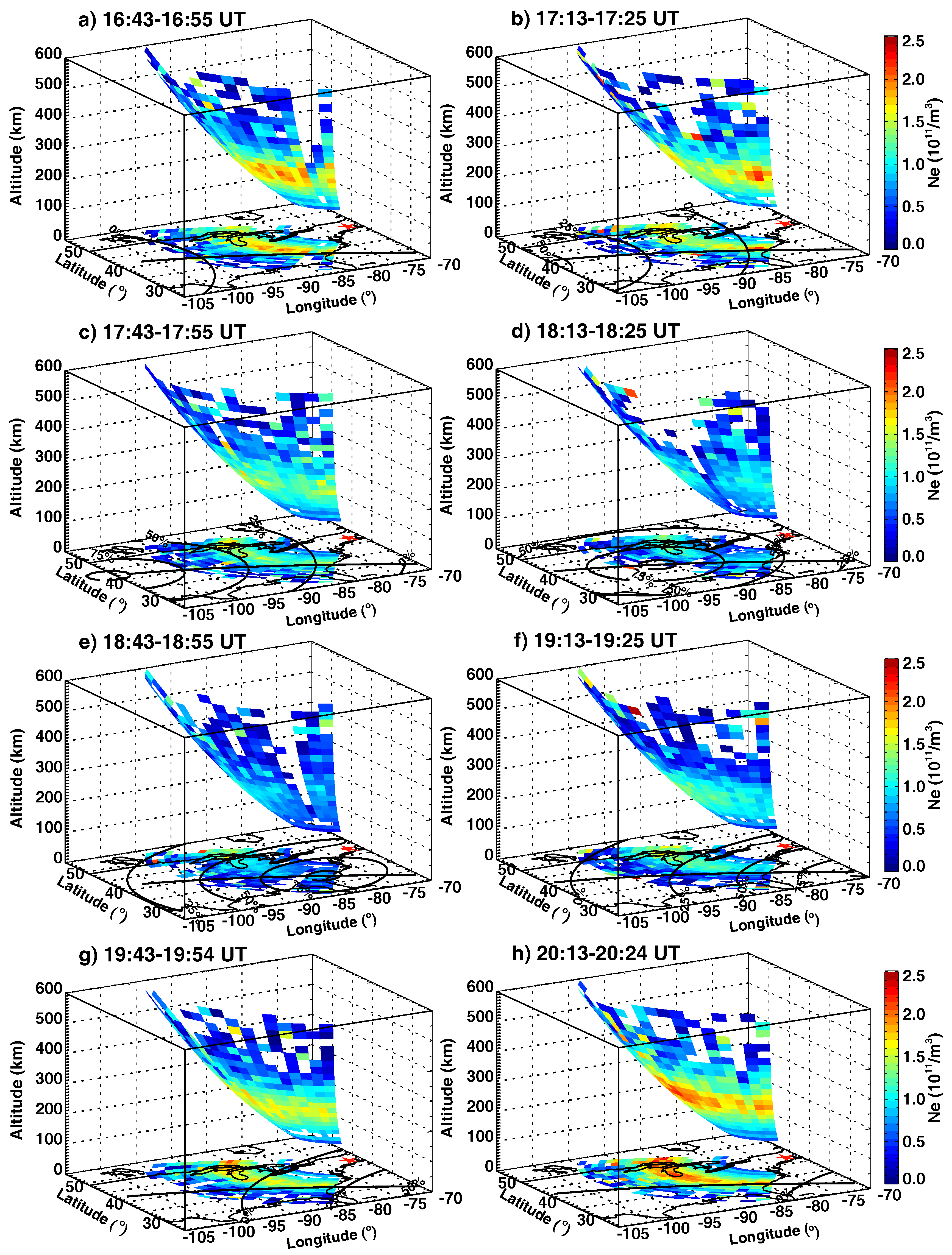
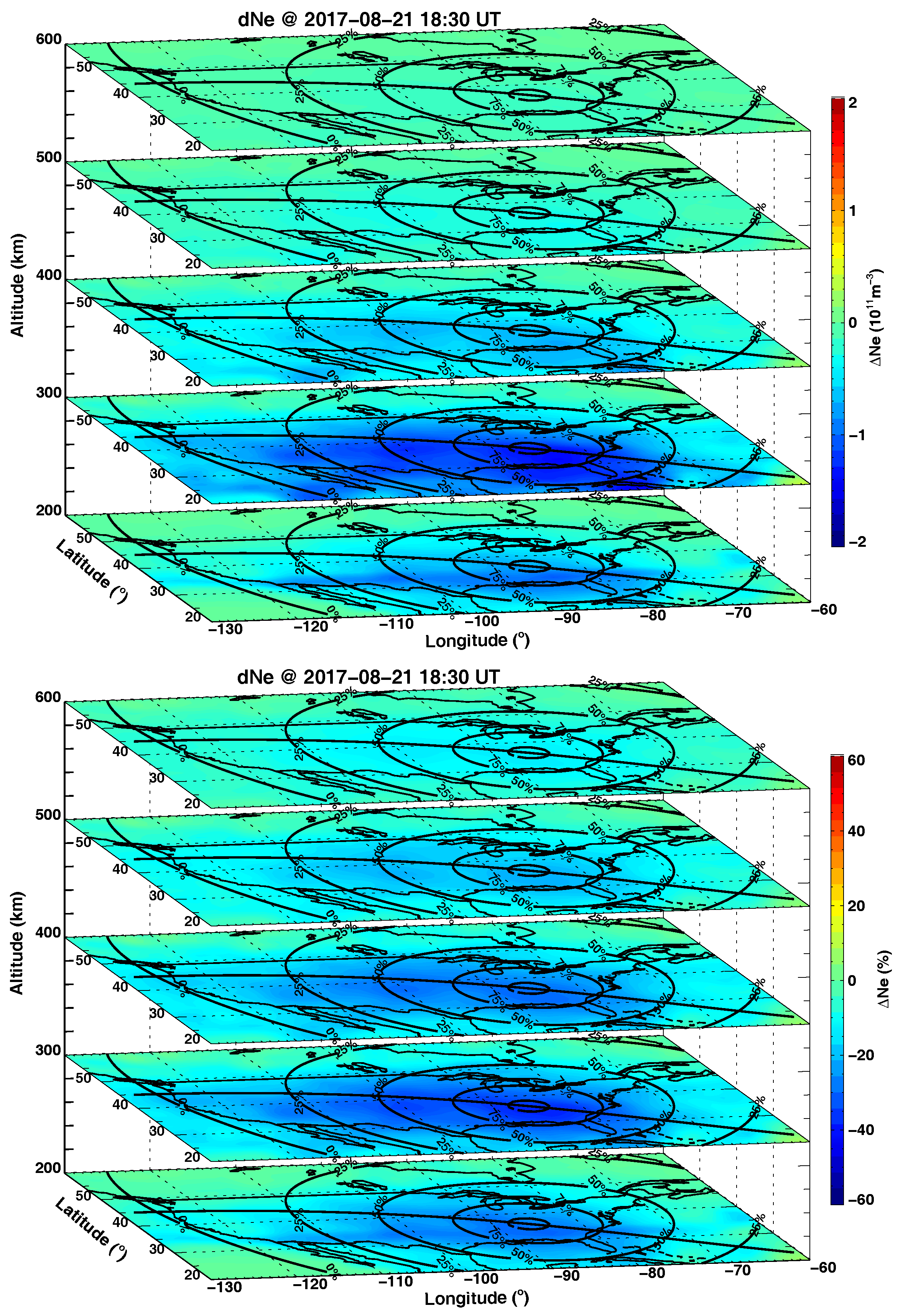
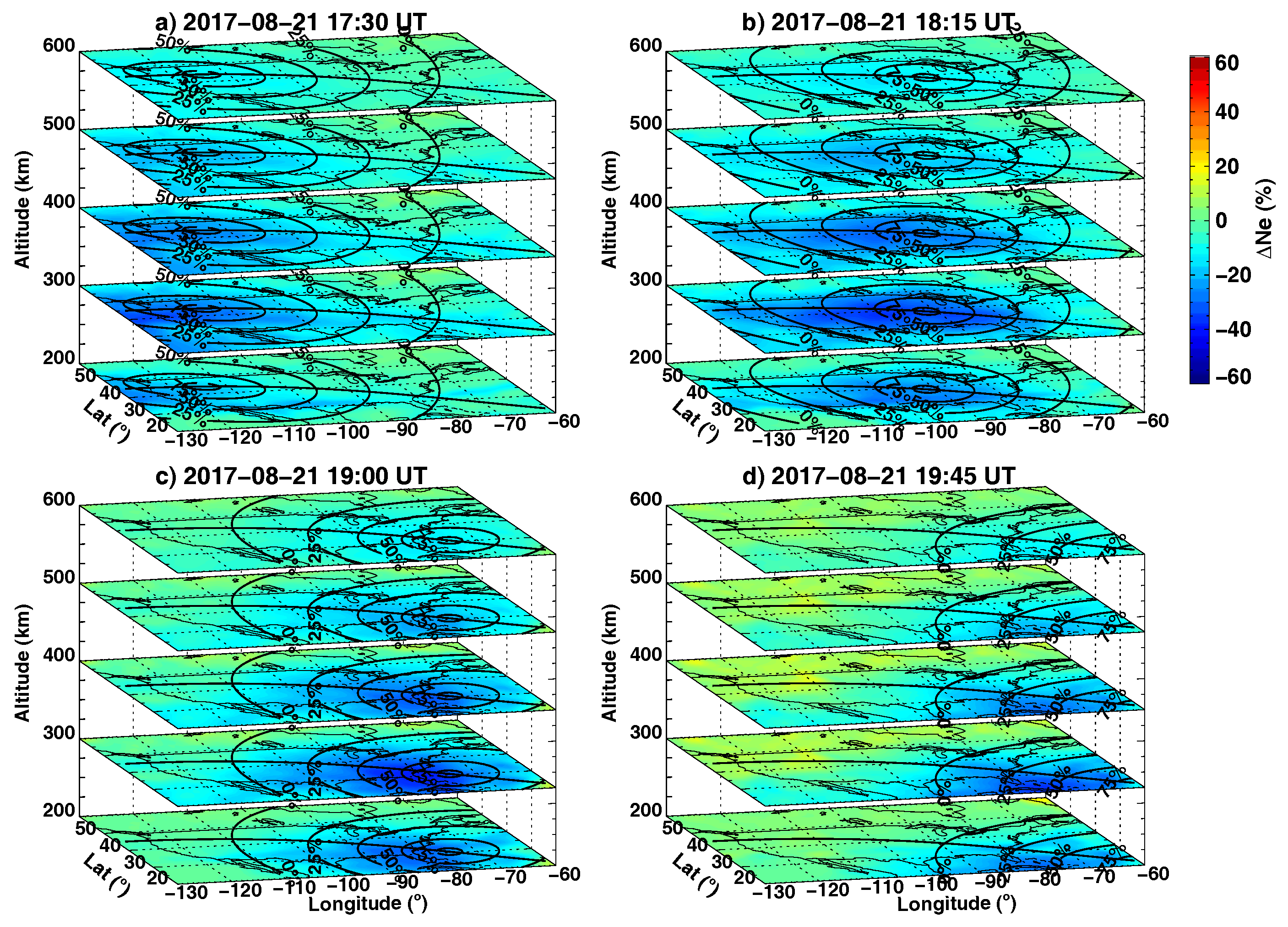
The high-resolution TIDAS products effectively reconstruct the 3-D ionospheric electron density variation during the eclipse, providing important altitude information. This accurately captured the key features of eclipse-induced electron density reduction and the subsequent post-eclipse enhancement in the 3-D domain, which showcase intricate features with details at a finer scale.
(2)
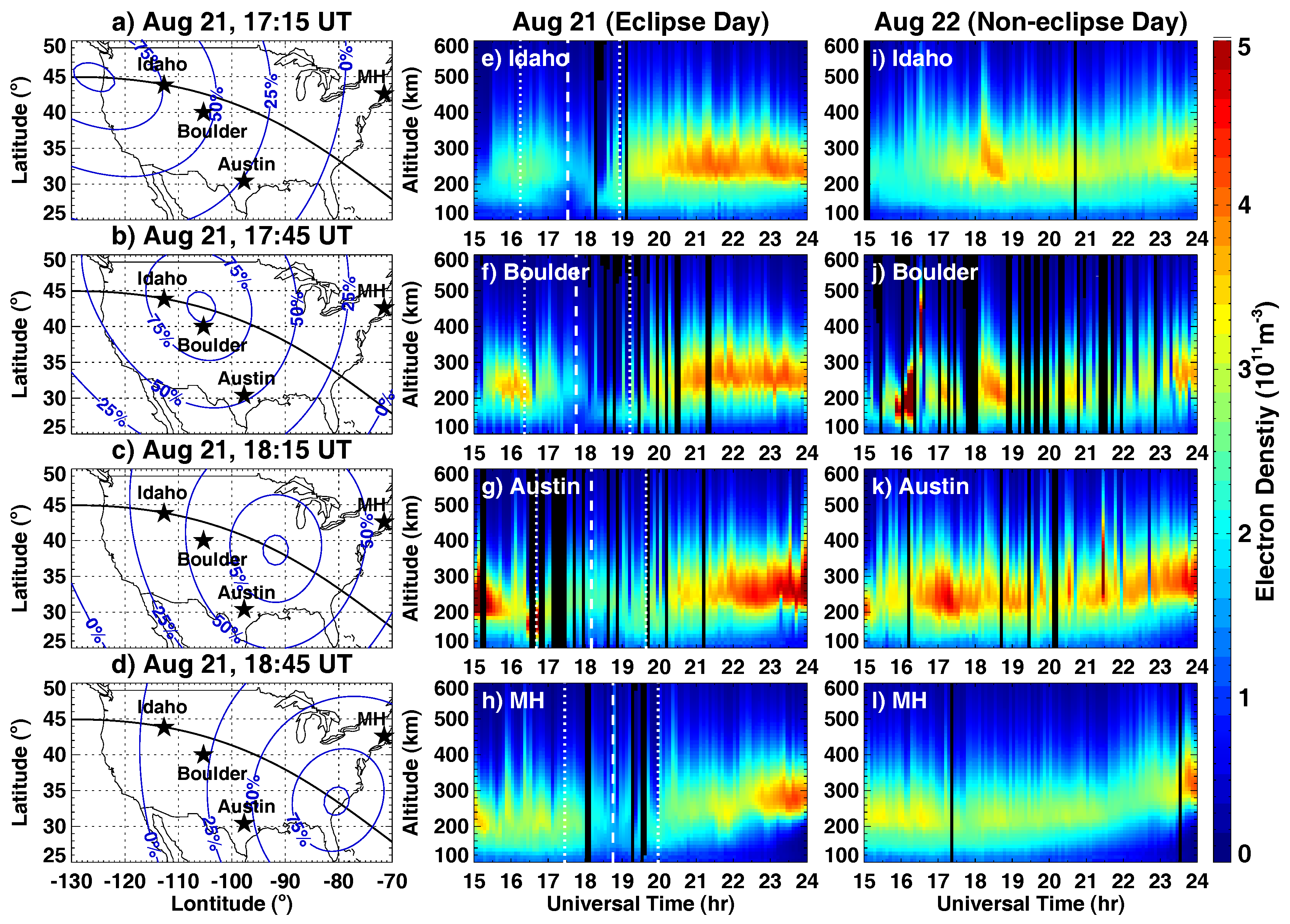
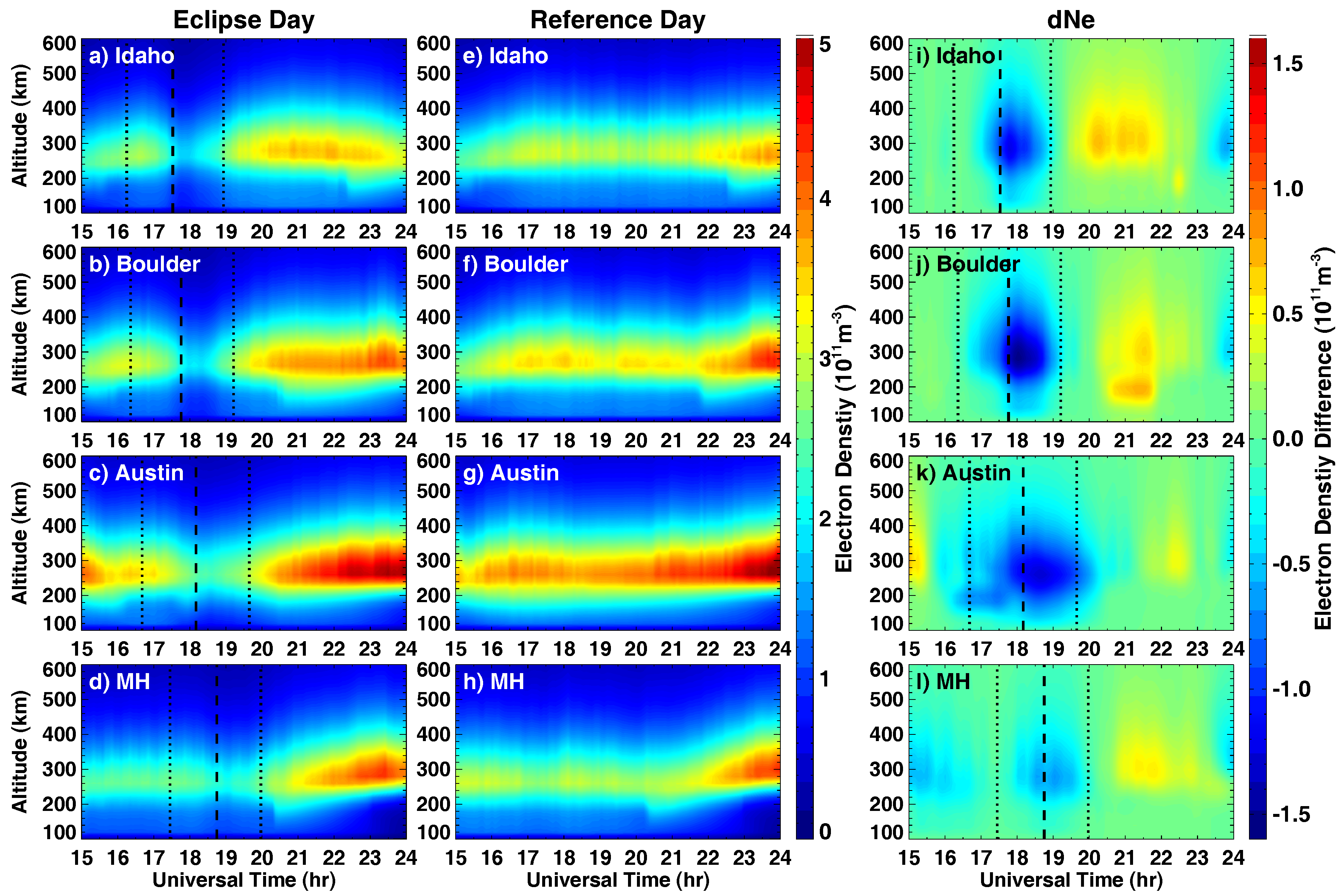
The combination of multi-instrumental observations and TIDAS results demonstrate that the eclipse-induced ionospheric electron density depletion exhibits an altitude-dependent feature. This reduction can exceed 50% in the F2 region, especially between altitudes of 200 and 300 km. Furthermore, the recovery of electron density after the end of depletion also exhibits an altitude-dependent behavior, where ionosphere at lower altitudes below 250 km exhibited a faster recovery than that at and above the F2 peak height. This is because the recovery in the photo-ionization rate has a more significant impact on the photo-chemical equilibrium at lower altitude ionosphere.
(3)
The multi-instrumental observations and TIDAS data assimilation results revealed the feature of post-eclipse electron density enhancement of 15–30%. This enhancement is more noticeable in the topside ionosphere, above the F2 peak height at altitudes higher than 300 km, especially in midlatitude regions at the poleward of the totality path. It is likely that this enhancement was primarily influenced by the downward plasma flux associated with the eclipse and the accompanying disruption caused by neutral winds.
In summary, this work successfully captured the key features of eclipse-induced electron density reduction and post-eclipse enhancement in the 3-D domain with important altitude information and fine-scale details, which has important implications for advancing current understanding of ionospheric changes and underlying mechanisms. In the future, continued efforts should be devoted in developing operational capabilities of 3-D ionospheric imaging to serve the needs of both research and space weather applications. The ultimate goal is to establish a robust, accurate, and timely ionospheric 3-D nowcast/forecast system to improve space weather specification, aiding in a quantitative assessment of the ionospheric weather effects caused by forthcoming solar eclipses and other geospace disturbances.

Author Contributions

Conceptualization, E.A. and S.-R.Z.; methodology, E.A.; software, E.A.; validation, E.A., S.-R.Z. and A.J.C.; formal analysis, E.A.; investigation, E.A.; resources, A.J.C.; writing—original draft preparation, E.A.; writing—review and editing, S.-R.Z., W.W. and A.J.C.; visualization, E.A.; supervision, S.-R.Z.; project administration, S.-R.Z.; funding acquisition, S.-R.Z. and P.J.E. All authors have read and agreed to the published version of the manuscript.

Funding

This work is supported by NSF awards AGS-1952737, AGS-2033787, AGS-2033843, AGS-2149698, and PHY-2028125, NASA support 80NSSC22K0171, 80NSSC21K1310, 80NSSC21K1775, 80NSSC19K0834, and 80GSFC22CA011, AFOSR MURI Project FA9559-16-1-0364, and ONR Grant N00014-17-1-2186 and N00014-22-1-2284. This work is also supported by the NASA contract 80GSFC18C0061 to the University of Colorado and by the NASA DRIVE Science Center for Geospace Storms (CGS) under award 80NSSC22M0163.

Data Availability Statement

Millstone Hill incoherent scatter radar observations are provided to the community through the Madrigal distributed data system at (http://cedar.openmadrigal.org/ (accessed on 1 July 2023)) by the Massachusetts Institute of Technology (MIT). The ionosonde data are provided by the University of Massachusetts Lowell DIDB database of Global Ionospheric Radio Observatory (https://giro.uml.edu/didbase/scaled.php (accessed on 1 July 2023)). The Swarm data are provided by European Space Agency (https://swarm-diss.eo.esa.int/ (accessed on 1 July 2023)).

Conflicts of Interest

The authors declare no conflict of interest.

References

  1. Rishbeth, H. Solar Eclipses and Ionospheric Theory. Space Sci. Rev. 1968, 8, 543–554. [Google Scholar] [CrossRef]
  2. Afraimovich, E.L.; Palamartchouk, K.S.; Perevalova, N.P.; Chernukhov, V.V.; Lukhnev, A.V.; Zalutsky, V.T. Ionospheric effects of the solar eclipse of March 9, 1997, as deduced from GPS data. Geophys. Res. Lett. 1998, 25, 465–468. [Google Scholar] [CrossRef]
  3. Coster, A.J.; Goncharenko, L.; Zhang, S.R.; Erickson, P.J.; Rideout, W.; Vierinen, J. GNSS Observations of Ionospheric Variations During the 21 August 2017 Solar Eclipse. Geophys. Res. Lett. 2017, 44, 12041–12048. [Google Scholar] [CrossRef]
  4. Ding, F.; Wan, W.; Ning, B.; Liu, L.; Le, H.; Xu, G.; Wang, M.; Li, G.; Chen, Y.; Ren, Z.; et al. GPS TEC response to the 22 July 2009 total solar eclipse in East Asia. J. Geophys. Res. Space Phys. 2010, 115, A07308. [Google Scholar] [CrossRef]
  5. Hoque, M.M.; Wenzel, D.; Jakowski, N.; Gerzen, T.; Berdermann, J.; Wilken, V.; Kriegel, M.; Sato, H.; Borries, C.; Minkwitz, D. Ionospheric response over Europe during the solar eclipse of March 20, 2015. J. Space Weather Space Clim. 2016, 6, A36. [Google Scholar] [CrossRef]
  6. Jakowski, N.; Stankov, S.M.; Wilken, V.; Borries, C.; Altadill, D.; Chum, J.; Buresova, D.; Boska, J.; Sauli, P.; Hruska, F.; et al. Ionospheric behavior over Europe during the solar eclipse of 3 October 2005. J. Atmos. Sol.-Terr. Phys. 2008, 70, 836–853. [Google Scholar] [CrossRef]
  7. Salah, J.E.; Oliver, W.L.; Foster, J.C.; Holt, J.M.; Emery, B.A.; Roble, R.G. Observations of the May 30, 1984, annular solar eclipse at Millstone Hill. J. Geophys. Res. 1986, 91, 1651–1660. [Google Scholar] [CrossRef]
  8. Tsai, H.F.; Liu, J.Y. Ionospheric total electron content response to solar eclipses. J. Geophys. Res. 1999, 104, 12657–12668. [Google Scholar] [CrossRef]
  9. Evans, J.V. On the behavior of foF2 during solar eclipses. J. Geophys. Res. 1965, 70, 733–738. [Google Scholar] [CrossRef]
  10. Goncharenko, L.P.; Erickson, P.J.; Zhang, S.R.; Galkin, I.; Coster, A.J.; Jonah, O.F. Ionospheric Response to the Solar Eclipse of 21 August 2017 in Millstone Hill (42N) Observations. Geophys. Res. Lett. 2018, 45, 4601–4609. [Google Scholar] [CrossRef]
  11. Hairston, M.R.; Mrak, S.; Coley, W.R.; Burrell, A.; Holt, B.; Perdue, M.; Depew, M.; Power, R. Topside Ionospheric Electron Temperature Observations of the 21 August 2017 Eclipse by DMSP Spacecraft. Geophys. Res. Lett. 2018, 45, 7242–7247. [Google Scholar] [CrossRef]
  12. MacPherson, B.; González, S.A.; Sulzer, M.P.; Bailey, G.J.; Djuth, F.; Rodriguez, P. Measurements of the topside ionosphere over Arecibo during the total solar eclipse of February 26, 1998. J. Geophys. Res. 2000, 105, 23055–23068. [Google Scholar] [CrossRef]
  13. Wang, W.; Dang, T.; Lei, J.; Zhang, S.; Zhang, B.; Burns, A. Physical Processes Driving the Response of the F2 Region Ionosphere to the 21 August 2017 Solar Eclipse at Millstone Hill. J. Geophys. Res. Space Phys. 2019, 124, 2978–2991. [Google Scholar] [CrossRef]
  14. Huba, J.D.; Drob, D. SAMI3 prediction of the impact of the 21 August 2017 total solar eclipse on the ionosphere/plasmasphere system. Geophys. Res. Lett. 2017, 44, 5928–5935. [Google Scholar] [CrossRef]
  15. Yau, A.W.; Foss, V.; Howarth, A.D.; Perry, G.W.; Watson, C.; Huba, J. Eclipse-Induced Changes to Topside Ion Composition and Field-Aligned Ion Flows in the August 2017 Solar Eclipse: E-POP Observations. Geophys. Res. Lett. 2018, 45, 10829–10837. [Google Scholar] [CrossRef]
  16. Aa, E.; Zhang, S.R.; Erickson, P.J.; Goncharenko, L.P.; Coster, A.J.; Jonah, O.F.; Lei, J.; Huang, F.; Dang, T.; Liu, L. Coordinated Ground-Based and Space-Borne Observations of Ionospheric Response to the Annular Solar Eclipse on 26 December 2019. J. Geophys. Res. Space Phys. 2020, 125, e28296. [Google Scholar] [CrossRef]
  17. Chen, C.H.; Lin, C.H.C.; Matsuo, T. Ionospheric responses to the 21 August 2017 solar eclipse by using data assimilation approach. Prog. Earth Planet. Sci. 2019, 6, 13. [Google Scholar] [CrossRef]
  18. Choudhary, R.K.; St.-Maurice, J.P.; Ambili, K.M.; Sunda, S.; Pathan, B.M. The impact of the January 15, 2010, annular solar eclipse on the equatorial and low latitude ionospheric densities. J. Geophys. Res. Space Phys. 2011, 116, A09309. [Google Scholar] [CrossRef]
  19. Harding, B.J.; Drob, D.P.; Buriti, R.A.; Makela, J.J. Nightside Detection of a Large-Scale Thermospheric Wave Generated by a Solar Eclipse. Geophys. Res. Lett. 2018, 45, 3366–3373. [Google Scholar] [CrossRef]
  20. Müller-Wodarg, I.C.F.; Aylward, A.D.; Lockwood, M. Effects of a mid-latitude solar eclipse on the thermosphere and ionosphere—A modelling study. Geophys. Res. Lett. 1998, 25, 3787–3790. [Google Scholar] [CrossRef]
  21. St.-Maurice, J.P.; Ambili, K.M.; Choudhary, R.K. Local electrodynamics of a solar eclipse at the magnetic equator in the early afternoon hours. Geophys. Res. Lett. 2011, 38, L04102. [Google Scholar] [CrossRef]
  22. Liu, J.Y.; Sun, Y.Y.; Kakinami, Y.; Chen, C.H.; Lin, C.H.; Tsai, H.F. Bow and stern waves triggered by the Moon’s shadow boat. Geophys. Res. Lett. 2011, 38, L17109. [Google Scholar] [CrossRef]
  23. Zhang, S.R.; Erickson, P.J.; Goncharenko, L.P.; Coster, A.J.; Rideout, W.; Vierinen, J. Ionospheric Bow Waves and Perturbations Induced by the 21 August 2017 Solar Eclipse. Geophys. Res. Lett. 2017, 44, 12067–12073. [Google Scholar] [CrossRef]
  24. Altadill, D.; Solé, J.G.; Apostolov, E.M. Vertical structure of a gravity wave like oscillation in the ionosphere generated by the solar eclipse of August 11, 1999. J. Geophys. Res. 2001, 106, 21419–21428. [Google Scholar] [CrossRef]
  25. Lin, C.Y.; Deng, Y.; Ridley, A. Atmospheric Gravity Waves in the Ionosphere and Thermosphere During the 2017 Solar Eclipse. Geophys. Res. Lett. 2018, 45, 5246–5252. [Google Scholar] [CrossRef]
  26. Nayak, C.; Yiǧit, E. GPS-TEC Observation of Gravity Waves Generated in the Ionosphere During 21 August 2017 Total Solar Eclipse. J. Geophys. Res. Space Phys. 2018, 123, 725–738. [Google Scholar] [CrossRef]
  27. Le, H.; Liu, L.; Ren, Z.; Chen, Y.; Zhang, H. Effects of the 21 June 2020 Solar Eclipse on Conjugate Hemispheres: A Modeling Study. J. Geophys. Res. Space Phys. 2020, 125, e28344. [Google Scholar] [CrossRef]
  28. Aa, E.; Zhang, S.R.; Shen, H.; Liu, S.; Li, J. Local and conjugate ionospheric total electron content variation during the 21 June 2020 solar eclipse. Adv. Space Res. 2021, 68, 3435–3454. [Google Scholar] [CrossRef]
  29. Zhang, S.R.; Erickson, P.J.; Vierinen, J.; Aa, E.; Rideout, W.; Coster, A.J.; Goncharenko, L.P. Conjugate Ionospheric Perturbation During the 2017 Solar Eclipse. J. Geophys. Res. Space Phys. 2021, 126, e28531. [Google Scholar] [CrossRef]
  30. Cherniak, I.; Zakharenkova, I. Ionospheric Total Electron Content Response to the Great American Solar Eclipse of 21 August 2017. Geophys. Res. Lett. 2018, 45, 1199–1208. [Google Scholar] [CrossRef]
  31. He, L.; Heki, K.; Wu, L. Three-Dimensional and Trans-Hemispheric Changes in Ionospheric Electron Density Caused by the Great Solar Eclipse in North America on 21 August 2017. Geophys. Res. Lett. 2018, 45, 10933–10940. [Google Scholar] [CrossRef]
  32. Liu, J.Y.; Wu, T.Y.; Sun, Y.Y.; Pedatella, N.M.; Lin, C.Y.; Chang, L.C.; Chiu, Y.C.; Lin, C.H.; Chen, C.H.; Chang, F.Y.; et al. Lunar Tide Effects on Ionospheric Solar Eclipse Signatures: The August 21, 2017 Event as an Example. J. Geophys. Res. Space Phys. 2020, 125, e28472. [Google Scholar] [CrossRef]
  33. Mrak, S.; Semeter, J.; Nishimura, Y.; Hirsch, M.; Sivadas, N. Coincidental TID Production by Tropospheric Weather During the August 2017 Total Solar Eclipse. Geophys. Res. Lett. 2018, 45, 10903–10911. [Google Scholar] [CrossRef]
  34. Sun, Y.Y.; Liu, J.Y.; Lin, C.C.H.; Lin, C.Y.; Shen, M.H.; Chen, C.H.; Chen, C.H.; Chou, M.Y. Ionospheric Bow Wave Induced by the Moon Shadow Ship Over the Continent of United States on 21 August 2017. Geophys. Res. Lett. 2018, 45, 538–544. [Google Scholar] [CrossRef]
  35. Pradipta, R.; Yizengaw, E.; Doherty, P. Ionospheric Density Irregularities, Turbulence, and Wave Disturbances During the Total Solar Eclipse Over North America on 21 August 2017. Geophys. Res. Lett. 2018, 45, 7909–7917. [Google Scholar] [CrossRef]
  36. Reinisch, B.W.; Dandenault, P.B.; Galkin, I.A.; Hamel, R.; Richards, P.G. Investigation of the Electron Density Variation During the 21 August 2017 Solar Eclipse. Geophys. Res. Lett. 2018, 45, 1253–1261. [Google Scholar] [CrossRef]
  37. Aryal, S.; Geddes, G.; Finn, S.C.; Mrak, S.; Galkin, I.; Cnossen, I.; Cook, T.; Chakrabarti, S. Multispectral and Multi-instrument Observation of TIDs Following the Total Solar Eclipse of 21 August 2017. J. Geophys. Res. Space Phys. 2019, 124, 3761–3774. [Google Scholar] [CrossRef]
  38. Perry, G.W.; Watson, C.; Howarth, A.D.; Themens, D.R.; Foss, V.; Langley, R.B.; Yau, A.W. Topside Ionospheric Disturbances Detected Using Radio Occultation Measurements During the August 2017 Solar Eclipse. Geophys. Res. Lett. 2019, 46, 7069–7078. [Google Scholar] [CrossRef]
  39. Uma, G.; Brahmanandam, P.S.; Srinivasu, V.K.D.; Prasad, D.S.V.V.D.; Sai Gowtam, V.; Tulasi Ram, S.; Chu, Y.H. Ionospheric responses to the 21 August 2017 great American solar eclipse—A multi-instrument study. Adv. Space Res. 2020, 65, 74–85. [Google Scholar] [CrossRef]
  40. Cnossen, I.; Ridley, A.J.; Goncharenko, L.P.; Harding, B.J. The Response of the Ionosphere-Thermosphere System to the 21 August 2017 Solar Eclipse. J. Geophys. Res. Space Phys. 2019, 124, 7341–7355. [Google Scholar] [CrossRef]
  41. Dang, T.; Lei, J.; Wang, W.; Zhang, B.; Burns, A.; Le, H.; Wu, Q.; Ruan, H.; Dou, X.; Wan, W. Global Responses of the Coupled Thermosphere and Ionosphere System to the August 2017 Great American Solar Eclipse. J. Geophys. Res. Space Phys. 2018, 123, 7040–7050. [Google Scholar] [CrossRef]
  42. Lei, J.; Dang, T.; Wang, W.; Burns, A.; Zhang, B.; Le, H. Long-Lasting Response of the Global Thermosphere and Ionosphere to the 21 August 2017 Solar Eclipse. J. Geophys. Res. Space Phys. 2018, 123, 4309–4316. [Google Scholar] [CrossRef]
  43. Wu, C.; Ridley, A.J.; Goncharenko, L.; Chen, G. GITM-Data Comparisons of the Depletion and Enhancement During the 2017 Solar Eclipse. Geophys. Res. Lett. 2018, 45, 3319–3327. [Google Scholar] [CrossRef]
  44. Yan, M.; Dang, T.; Lei, J.; Wang, W.; Zhang, S.R.; Le, H. From Bow Waves to Traveling Atmospheric Disturbances: Thermospheric Perturbations Along Solar Eclipse Trajectory. J. Geophys. Res. Space Phys. 2021, 126, e28523. [Google Scholar] [CrossRef]
  45. Aa, E.; Forsythe, V.V.; Zhang, S.R.; Wang, W.; Coster, A.J. Next-decade needs for 3-D ionosphere imaging. Front. Astron. Space Sci. 2023, 10, 1186513. [Google Scholar] [CrossRef]
  46. Chen, C.H.; Lin, C.C.H.; Lee, C.J.; Liu, J.Y.; Saito, A. Ionospheric responses on the 21 August 2017 solar eclipse by using three-dimensional GNSS tomography. Earth Planets Space 2022, 74, 173. [Google Scholar] [CrossRef]
  47. Lin, C.Y.; Liu, J.Y.; Lin, C.C.H.; Chou, M.Y. The Ionospheric Three-Dimensional Electron Density Variations Induced by the 21 August 2017 Total Solar Eclipse by Using Global Ionospheric Specification. Remote Sens. 2023, 15, 3887. [Google Scholar] [CrossRef]
  48. Aa, E.; Zhang, S.R.; Erickson, P.J.; Wang, W.; Coster, A.J.; Rideout, W. 3-D Regional Ionosphere Imaging and SED Reconstruction With a New TEC-Based Ionospheric Data Assimilation System (TIDAS). Space Weather 2022, 20, e2022SW003055. [Google Scholar] [CrossRef]
  49. Aa, E.; Erickson, P.J.; Zhang, S.R.; Zou, S.; Coster, A.J.; Goncharenko, L.P.; Foster, J.C. A Statistical Study of the Subauroral Polarization Stream Over North American Sector Using the Millstone Hill Incoherent Scatter Radar 1979–2019 Measurements. J. Geophys. Res. Space Phys. 2020, 125, e28584. [Google Scholar] [CrossRef]
  50. Erickson, P.J.; Beroz, F.; Miskin, M.Z. Statistical characterization of the American sector subauroral polarization stream using incoherent scatter radar. J. Geophys. Res. Space Phys. 2011, 116, A00J21. [Google Scholar] [CrossRef]
  51. Foster, J.C.; Vo, H.B. Average characteristics and activity dependence of the subauroral polarization stream. J. Geophys. Res. Space Phys. 2002, 107, 1475. [Google Scholar] [CrossRef]
  52. Zhang, S.R.; Holt, J.M. Ionospheric plasma temperatures during 1976–2001 over Millstone Hill. Adv. Space Res. 2004, 33, 963–969. [Google Scholar] [CrossRef]
  53. Rideout, W.; Coster, A. Automated GPS processing for global total electron content data. GPS Solut. 2006, 10, 219–228. [Google Scholar] [CrossRef]
  54. Brunini, C.; Meza, A.; Bosch, W. Temporal and spatial variability of the bias between TOPEX- and GPS-derived total electron content. J. Geod. 2005, 79, 175–188. [Google Scholar] [CrossRef]
  55. Nava, B.; Coïsson, P.; Radicella, S.M. A new version of the NeQuick ionosphere electron density model. J. Atmos. Sol.-Terr. Phys. 2008, 70, 1856–1862. [Google Scholar] [CrossRef]
  56. Bust, G.S.; Garner, T.W.; Gaussiran, T.L. Ionospheric Data Assimilation Three-Dimensional (IDA3D): A global, multisensor, electron density specification algorithm. J. Geophys. Res. Space Phys. 2004, 109, A11312. [Google Scholar] [CrossRef]
  57. Forsythe, V.V.; Azeem, I.; Blay, R.; Crowley, G.; Gasperini, F.; Hughes, J.; Makarevich, R.A.; Wu, W. Evaluation of the New Background Covariance Model for the Ionospheric Data Assimilation. Radio Sci. 2021, 56, e2021RS007286. [Google Scholar] [CrossRef]
  58. Aa, E.; Zhang, S.R.; Wang, W.; Erickson, P.J.; Coster, A.J. Multiple longitude sector storm-enhanced density (SED) and long-lasting subauroral polarization stream (SAPS) during the 26–28 February 2023 geomagnetic storm. J. Geophys. Res. Space Phys. 2023, 128, e2023JA031815. [Google Scholar] [CrossRef]
  59. Belehaki, A.; Moratis, G.; Tsagouri, I. On the derivation of an hourly local index to define the normal ionosphere. Ann. Geophys. 2000, 43, 189–203. [Google Scholar] [CrossRef]
  60. Bojilova, R.; Mukhtarov, P. Global and Regional Response of the Total Electron Content to Geomagnetic Storms Occurred in January 2005. In Proceedings of the Eleventh Workshop on Solar Influences on the Magnetosphere, Ionosphere and Atmosphere, Primorsko, Bulgaria, 3–7 June 2019; Georgieva, K., Kirov, B., Danov, D., Eds.; Space Research and Technologies Institute: Sofia, Bulgaria, 2019; pp. 71–76. [Google Scholar] [CrossRef]
  61. Reinisch, B.W.; Huang, X. Deducing topside profiles and total electron content from bottomside ionograms. Adv. Space Res. 2001, 27, 23–30. [Google Scholar] [CrossRef]
  62. Le, H.; Liu, L.; Yue, X.; Wan, W.; Ning, B. Latitudinal dependence of the ionospheric response to solar eclipses. J. Geophys. Res. Space Phys. 2009, 114, A07308. [Google Scholar] [CrossRef]
  63. Le, H.; Liu, L.; Yue, X.; Wan, W. The midlatitude F2 layer during solar eclipses: Observations and modeling. J. Geophys. Res. 2008, 113, A08309. [Google Scholar] [CrossRef]
  64. Rishbeth, H.; Jenkins, B.; Moffett, R.J. The F-layer at sunrise. Ann. Geophys. 1995, 13, 367–374. [Google Scholar] [CrossRef]
Figure 1. (ah) Three-dimensional electron density profiles of the Millstone Hill incoherent scatter radar (red star) for the wide azimuth scan and the corresponding 2-D projection map using the same longitude/latitude information on 21 August 2017. The totality path of the solar eclipse and the 0%, 25%, 50%, 75%, and 95% obscuration lines are plotted on the bottom surface.
Atmosphere 14 01379 g001
Figure 2. (ad) The continental US maps with the eclipse totality path and the 0%, 25%, 50%, 75%, and 95% obscuration lines at four UT intervals between 17:15 and 18:45 UT on 21 August 2017. The locations of four ionosondes are marked with stars. (el) Comparison of ionosonde electron density profiles between 15 and 24 UT on the eclipse day (21 August) and the day after (22 August). The local eclipse start, maximum, and end times are marked with vertical white lines.
Atmosphere 14 01379 g002
Figure 3. (ah) Comparison of TIDAS reconstructed electron density profiles at four ionosonde locations between 15 and 24 UT on the eclipse day (21 August) and the reference day (22 August). (il) The electron density difference between the eclipse day and reference day. The local eclipse start, maximum, and end times are marked with vertical lines.
Atmosphere 14 01379 g003
Figure 4. Three-dimensional distribution of the absolute (upper panels) and percentage (bottom panels) dNe maps reconstructed by TIDAS data assimilation between 200 and 600 km at 18:30 UT on 21 August 2017. The eclipse totality path and different obscuration zones of 95%, 75%, 50%, 25%, and 0% are plotted.
Atmosphere 14 01379 g004
Figure 5. (ad) Three-dimensional distribution of the reconstructed dNe maps given by TIDAS data assimilation at eight UT intervals between 17:30 and 19:45 UT. The eclipse totality path and different obscuration zones of 95%, 75%, 50%, 25%, and 0% are plotted.
Atmosphere 14 01379 g005
Figure 6. (ad) The same as Figure 5 but for 3-D distribution of percentage dNe maps.
Atmosphere 14 01379 g006
Figure 7. (ad) Two-dimensional regional maps of reanalyzed dTEC and dNmF2 (F2-layer peak density) given by TIDAS data assimilation between 17:15 and 19:30 UT on 21 August 2017. The eclipse totality path and different obscuration zones of 95%, 75%, 50%, 25%, and 0% are plotted.
Atmosphere 14 01379 g007
Figure 8. (ad) TIDAS-derived 2-D dNe maps at 450 km and dTEC maps overlapping with the Swarm C satellite orbits (red lines) at 18:40 UT and 20:10 UT on 21 August 2017. The eclipse totality path and different obscuration zones are plotted. The right subpanels show the corresponding latitudinal profiles of Ne or TEC given by Swarm C (red) and TIDAS (black), as compared with the reference values on 22 August 2017 (dotted lines).
Atmosphere 14 01379 g008
Disclaimer/Publisher’s Note: The statements, opinions and data contained in all publications are solely those of the individual author(s) and contributor(s) and not of MDPI and/or the editor(s). MDPI and/or the editor(s) disclaim responsibility for any injury to people or property resulting from any ideas, methods, instructions or products referred to in the content.

