Article

An Assessment of Global Dimming and Brightening during 1984–2018 Using the FORTH Radiative Transfer Model and ISCCP Satellite and MERRA-2 Reanalysis Data

by
Michael Stamatis
1,
Nikolaos Hatzianastassiou
1,*,
Marios-Bruno Korras-Carraca
1,2,
Christos Matsoukas
3,
Martin Wild
4 and
Ilias Vardavas
5
1
Laboratory of Meteorology & Climatology, Department of Physics, University of Ioannina, 45110 Ioannina, Greece
2
Institute for Astronomy, Astrophysics, Space Applications and Remote Sensing, National Observatory of Athens, 11810 Athens, Greece
3
Department of Environment, University of the Aegean, 81100 Mytilene, Greece
4
Institute for Atmospheric and Climate Science, ETH Zürich, 8092 Zürich, Switzerland
5
Department of Physics, University of Crete, 71003 Heraklion, Greece
*
Author to whom correspondence should be addressed.
Atmosphere 2023, 14(8), 1258; https://doi.org/10.3390/atmos14081258
Submission received: 15 July 2023 / Revised: 2 August 2023 / Accepted: 3 August 2023 / Published: 8 August 2023

Abstract

:
In this study, an assessment of the FORTH radiative transfer model (RTM) surface solar radiation (SSR) as well as its interdecadal changes (Δ(SSR)), namely global dimming and brightening (GDB), is performed during the 35-year period of 1984–2018. Furthermore, a thorough evaluation of SSR and (Δ(SSR)) is conducted against high-quality reference surface measurements from 1193 Global Energy Balance Archive (GEBA) and 66 Baseline Surface Radiation Network (BSRN) stations. For the first time, the FORTH-RTM Δ(SSR) was evaluated over an extended period of 35 years and with a spatial resolution of 0.5° × 0.625°. The RTM uses state-of-the-art input products such as MERRA-2 and ISCCP-H and computes 35-year-long monthly SSR and GDB, which are compared to a comprehensive dataset of reference measurements from GEBA and BSRN. Overall, the FORTH-RTM deseasonalized SSR anomalies correlate satisfactorily with either GEBA (R equal to 0.72) or BSRN (R equal to 0.80). The percentage of agreement between the sign of computed GEBA and FORTH-RTM Δ(SSR) is equal to 63.5% and the corresponding percentage for FORTH-RTM and BSRN is 54.5%. The obtained results indicate that a considerable and statistically significant increase in SSR (Brightening) took place over Europe, Mexico, Brazil, Argentina, Central and NW African areas, and some parts of the tropical oceans from the early 1980s to the late 2010s. On the other hand, during the same 35-year period, a strong and statistically significant decrease in SSR (Dimming) occurred over the western Tropical Pacific, India, Australia, Southern East China, Northern South America, and some parts of oceans. A statistically significant dimming at the 95% confidence level, equal to −0.063 Wm−2 year−1 (or −2.22 Wm−2) from 1984 to 2018 is found over the entire globe, which was more prevalent over oceanic than over continental regions (−0.07 Wm−2 year−1 and −0.03 Wm−2 year−1, statistically significant dimming at the 95% confidence level, respectively) in both hemispheres. Yet, this overall 35-year dimming arose from alternating decadal-scale changes, consisting of dimming during 1984–1989, brightening in the 1990s, turning into dimming over 2000–2009, and brightening during 2010–2018.

1. Introduction

Surface solar radiation (or SSR) is a significant component of the overall energy balance of the planet, regulating the Earth’s climate and determining its water cycle and general circulation, while it affects the carbon cycle and the photosynthesis of plants [1,2,3]. The late 1980s marked the beginning of the acknowledgment of existing interdecadal variations in SSR, referred to as global dimming and brightening (GDB) [4,5,6] and it has been demonstrated that clouds and aerosols, which greatly influence the transparency of the atmosphere, are the two main causes of GDB [6,7]. GDB may be a local or global phenomenon [6,7,8] and has effects on several areas, including the economy, agriculture [3], solar power, hydrology [9], and climate [10]. For instance, the study by [10] revealed that since the 1980s, the lack of solar dimming and its masking effects allowed greenhouse warming to become more apparent, leading to a more rapid increase in temperature than in prior decades. According to several studies analyzing surface solar radiation measurements, SSR decreased globally from the early 1960s to the late 1980s, a trend known as “global dimming” [8,11,12,13,14], but there has been no evidence of this trend continuing since the late 1980s at many locations. In fact, SSR increased during the 1990s, a trend known as “global brightening” [6,15,16,17]. However, solar dimming persisted across India and Southeast Asia until 2000 [18,19,20,21]. After the year 2000, it was found that the brightening across Europe and North America remained, whereas it leveled off at locations in Japan and the dimming continued in India and China [15].
Due to the large-scale GDB phenomenon, accurate inferences cannot be formed from surface measurements alone. The knowledge of the phenomenon from ground-based measurements should be supplemented by satellite observations/models and reanalysis datasets, which offer large and complete spatial, as well as temporal, coverage. However, since such datasets more or less involve theory, they have limited consistency in terms of trends and must be evaluated against ground-based measurements to ensure their reliability. Other reasons for such an evaluation are the detection of errors in cloud and aerosol input data to the models and inhomogeneities in the assimilated data records in reanalysis, which may cause possible uncertainties in the estimated fluxes [22,23,24,25,26,27]. Several studies using model simulations and/or satellite data [7,8,28,29,30,31,32,33,34] found that the dimming and brightening during the 1980s and 1990s, respectively, were global rather than local, whereas they also reported divergent trends in SSR even over neighboring regions. More specifically, the investigation by [8] based on the International Satellite Cloud Climatology Project-D2 series (ISCCP-D2) identified substantial increasing trends in SSR, i.e., brightening, between 1984 and 2000, yielding an average increase of 2.4 Wm−2 decade−1. Additionally, using satellite retrievals from ISCCP-D1, Ref. [31] computed a global brightening of 1.6 Wm−2 decade−1 between 1983 and 2001, which was associated with decreasing cloud cover fraction. According to the analysis performed by [32] using data from the Global Energy and Water Exchanges Project- Surface Radiation Budget version 2.8 (GEWEX-SRB V2.8), there was a dimming of −2.51 Wm−2 decade−1 between 1983 and 1991, a brightening of 3.17 Wm−2 decade−1 from 1991 to 1999, a subsequent dimming of −5.26 Wm−2 decade−1 during 1999–2004, and an overall brightening of 0.25 Wm−2 decade−1 during 1983–2004. Moreover, Ref. [28] calculated a global dimming of −2.0 Wm−2 from 1920 to 2000, which is in line with simulations from 10 models used in the Fourth Assessment Report (IPCC-AR4) of the United Nations Intergovernmental Panel on Climate Change (UNIPCC), which reported a dimming that is ranging in different models from −1 to −4 Wm−2 globally during the entire 20th century [35]. Moreover, they [28] noticed a dimming trend from 1968 to 1977, followed by a brightening trend in the 1980s and 1990s.
There were few attempts to extend GDB beyond 2000 and even fewer beyond 2010 using satellite-derived SSR, showing a tendency for dimming in the years following 2000. A study by [30] using a radiation transfer model with input from ISCCP-D2 satellite data for the years 2001–2006 revealed a just slight (0.17 Wm−2) brightening in the Northern Hemisphere and a dimming (−2.88 Wm−2) in the Southern Hemisphere, where dimming was primarily seen over the oceans and a slight brightening over land. The same authors [7], using the same radiative transfer model with input cloud data from ISCCP-D2, aerosol data from MODIS (Moderate Resolution Imaging Spectroradiometer) C006, and meteorological data from NCEP/NCAR (National Centers for Environmental Predictions and National Center for Atmospheric Research), during 2000–2009, computed an overall dimming, weaker in the Northern than in the Southern Hemisphere (−2.2 and −3.1 W m−2, respectively). According to that study, both land and ocean areas in either hemisphere showed dimming, but the one in Southern Hemisphere land was more prominent. Furthermore, using retrieved Clouds and the Earth’s Radiant Energy System (CERES) satellite SSR data for the years 2001 to 2012, Ref. [33] found a brightening equal to 0.03 Wm−2 decade−1. The same authors using GEWEX-SRB V3.0 and ISCCP-FD SSR data for the Globe, computed a significant dimming between 1984 and 1991, followed by a brightening from 1992 to 2000 and a return to significant dimming over 2001–2007. They also noticed a disagreement between ground-based records and satellite-derived products over China, suggesting that the differences between satellite estimates and surface measurements might have been related to aerosols, clouds, and their interactions as represented in the satellite algorithm, but also to questionable pyranometer’s accuracy and measurement methods. Moreover, Ref. [36], using the CM-SAF SARAH (Satellite Application Facility on Climate Monitoring Solar surfAce RAdiation Heliosat) satellite-based product, found that during 1983–2013 a brightening (0.2 ± 0.05 Wm−2 year−1) occurred in the southeastern Mediterranean, being similar over land and sea. Another study by [37] using SARAH-2 and CLARA-A2 (CM SAF cLoud, Albedo, and surface RAdiation dataset from AVHRR) computed an overall brightening in Europe since the 1980s, equal to 2.4 Wm−2 decade−1 at 53 European GEBA stations and 1.9 Wm−2 decade−1 at the corresponding SARAH-2 grid cells, with substantial decadal and spatial variability, during the period 1983–2015. Moreover, a study [38] using satellite-derived data over Europe (1983–2010) showed a widespread increase in SSR in a major part of Europe, especially in spring. Moreover, they reported a significant difference between the trends of ground-based and satellite observations, which is not explained by calibration issues of the satellite product alone. Additionally, Ref. [39] using satellite-derived products (ISCCP-FH) and reanalyses (ERA5 and NCEP-NCAR reanalysis II) show consistent increases in SSR and decreases in cloud cover over North America and Europe from the 1980s to the 2010s.
On the other hand, along with the satellite-derived products, reanalysis SSR datasets, which incorporate both observations and models, have also the benefit of offering complete spatial coverage and extensive temporal coverage, and as a result, they are frequently employed in atmospheric sciences and studies of climate change [22]. The interdecadal variation of various reanalysis SSR was computed and evaluated against ground-based stations over specific world regions, such as in China using Modern-Era Retrospective analysis for Research and Applications, version 2 (MERRA-2) by [26], in Europe using 20CRv2c, 20CRv3, ERA20C, and CERA20C by [40] or globally with MERRA-2 by [41]. It should be noted, however, that reanalysis products generally tend to overestimate the SSR [22,42] and further improvements are necessary for better representation of SSR trends [41], since they have difficulties reproducing the SSR trends [40,41].
An extension of the existing studies is attempted here, and a step forward is made in improving our knowledge about the ongoing GDB and its climatic role. An overall assessment of the GDB is attempted in the present work, studying it for the first time on a global scale and for the long climatological period of 1984–2018, also including very recent years not covered in the literature. The study is performed using the FORTH (Foundation for Research and Technology-Hellas) radiative transfer model (RTM) that also has been used in previous studies [7,8,30] and state-of-the-art cloud (ISCCP-H) and aerosol (MERRA-2) input data. To ensure the reliability of the obtained GDB over the 35-year period 1984–2018, a detailed evaluation of the RTM monthly SSR and GDB (changing SSR, i.e., Δ(SSR)) is performed through comparisons against ground-based observations from the reference GEBA and BSRN networks. The innovations of the present study in relation to our previous ones [7,8,30] are: (i) the higher spatial resolution of model SSR and GDB, computed on a 0.5° × 0.625° latitude-longitude grid over the entire globe, (ii) the quite long study period of 1984–2018, (iii) the coverage of recent years, up to 2018, (iv) the use of a large observational dataset, consisting of highest quality reference measurements, for the evaluation of SSR and GDB and (v) the use of state-of-the-art RTM input datasets, such ISCCP-H and MERRA-2. Additionally, a columnar closure study is carried out in which the long-term changes of FORTH-RTM reflected solar radiation fluxes at the Top of Atmosphere (TOA) are compared to the corresponding fluxes of CERES-EBAF, which are used as reference. This is performed in order to further strengthen the robustness of the derived conclusions and to achieve the maximum possible reliability of the computed GDB. Deseasonalized anomalies are used for the evaluation of the FORTH-RTM SSR and GDB at a variety of scales, from local (station-level) to global/hemispheric, and for temporal ranges spanning from the full 35-year study down to selected individual sub-periods. The data and methods that were used are described in Section 2; the results of the attempted evaluation are presented and discussed in Section 3; and lastly, conclusions and perspectives are given in Section 4.

2. Materials and Methods

2.1. Model and Data

2.1.1. FORTH Radiation Transfer Model

The utilized FORTH spectral radiative transfer model, which is described in detail in the works by [8,43,44], was developed from a radiative-convective model [45]. The atmosphere is discriminated into clear and cloudy (for low-, mid-, and high-level clouds) fractions. The RTM solves, for an absorbing/multiple-scattering atmosphere, the radiative transfer equations for 118 separate wavelengths for the ultraviolet-visible part of the solar spectrum (wavelengths between 0.2 and 1.0 μm), and for ten bands for the near-infrared part (between 1.0 and 10.0 μm), using the modified Delta-Eddington method of [46] that relies on the Henyey–Greenstein phase function, which is an extension of the Eddington method outlined in [47]. Rayleigh scattering, molecular absorption in the ultraviolet, visible and near-infrared, aerosol and cloud scattering and absorption, and surface reflection are all considered. More specifically, when applying the delta-Eddington method the physical parameters of optical thickness (τ), asymmetry parameter (g), and single-scattering albedo (ω), are replaced using the following transformations:
τ = 1 ω f τ
ω = 1 f ω 1 ω f
g = g 1 + g
where f = g2. The atmosphere is separated into distinct layers, each of which has a total optical thickness calculated as follows:
τ = τ a e r s + τ a e r a + τ m a + τ R + τ c s + τ c a
where τaers, τaera are, respectively, the scattering and absorption optical thicknesses of the aerosols, τma is the optical thickness of molecular absorption, τR the optical thickness of Rayleigh scattering, while τcs and τca are the scattering and absorption optical thicknesses, respectively, of the clouds. Single-scattering albedo for each layer is given by the following relation:
ω = ω a e r + ω R + ω c
where:
ω a e r = τ a e r s τ
ω R = τ R τ
ω c = τ c s τ
Finally, the asymmetry parameter of each layer of the model is calculated from the equation:
g = g a e r ω a e r + g R ω R + g c ω c ω
in which gaer is the aerosol asymmetry parameter, gc is the asymmetry parameter of clouds, and gR is the Rayleigh scattering asymmetry parameter (equal to 0, due to isotropic scattering of solar radiation from atmospheric gases). The temporal resolution of the current version of FORTH-RTM utilized here is monthly and the spatial resolution is 0.5° × 0.625° latitude x longitude. The cloud properties required by the model, namely cloud amount, cloud optical depth, and cloud-top pressure separately for liquid and ice phases, are taken from the ISCCP-H dataset. The aerosol optical depth, single scattering albedo, asymmetry parameter, specific humidity, ozone concentration, and surface albedo were computed from data taken from the MERRA-2 Reanalysis. All the original input data were converted to monthly means, and regridded to the 0.5° × 0.625° latitude-longitude spatial resolution, to be used in the RTM. The incoming solar irradiance at the top of atmosphere (TOA) is computed between 0.2–10.0 μm, based on the spectral profile of [48], using a solar constant S = 1367 Wm⁠−2, which is corrected for the Earth’s elliptical orbit. The mixing ratio of CH4 is set equal to 9 × 10⁻⁴ gcm−2 (or 1.7 parts per million by volume (ppmv)), CO2 equal to 0.58 gcm−2 (or 371 ppmv, the value of 2001), and N2O equal to 4.5 × 10⁻⁴ gcm−2 (or 0.3 ppmv). The output of the model consists of the upwelling and downwelling solar fluxes at the surface of the Earth, at 50 levels within the atmosphere, and at the top of the atmosphere. Solar fluxes are computed separately for the spectral regions of the ultraviolet-visible, near-infrared, and the entire spectrum (0.2–10 μm). In the current study, the downwelling at the Earth’s surface, shortwave solar radiation flux for the entire spectrum was used for the evaluation and GDB assessment.
In the following two Section 2.1.2 and Section 2.1.3 the RTM input data are briefly described, while in the following two Section 2.1.4 and Section 2.1.5 the data used for the evaluation of the RTM fluxes are presented.

2.1.2. ISCCP-H

The ISSCP-H climate data record contains the full (level 2) and basic (level 3) products for monitoring the distribution and variation of cloud and surface properties, which are derived from both geostationary and polar-orbiting satellite imaging radiometers with one visible (VIS ≈ 0.65 ± 0.05–0.20 μm) and one infrared (IR ≈ 10.5 ± 0.5–0.75 μm) “window” channels. The Basic H-series data that are used in this study currently span the period from July 1983 to December 2018 with plans for regular updates. They have global coverage with spatial resolution of 1° × 1° degree, equal angle grid. The improvements of the ISCCP H-series, compared to its predecessors C- and D-series are several and include quality control measures, modified ancillary inputs, higher spatial resolution input and output products, and calibration refinements [49]. The cloud types include 3 low-, 3 middle-, and 3 high-level cloud types, each one in liquid and ice phases, thus the overall number of ISCCP-H cloud types is 18. Here, the basic, monthly ISCCP H Gridded Monthly (HGM) data are used and more specifically the properties with names “cldamt_types”, “tau_types” and “pc_types” corresponding to the mean cloud amount, mean cloud-top pressure and mean cloud optical depth for 18 cloud types. The mean monthly data were computed by averaging each 3-hourly time step for a month and then by averaging the eight (8) 3-hourly mean values in the month. Due to the requirements of FORTH-RTM, the initial 1° × 1° gridded data, were regridded to 0.5° × 0.625° applying the first-order conservative remapping method [50] from the Climate Data Operators (CDO) with the “remapcon” command. All ISSCP-H data products are available in [51].

2.1.3. MERRA-2

The MERRA-2 is a state-of-the-art reanalysis produced by the NASA Global Modeling and Assimilation Office (GMAO) in 2017 [52]. Its advances in assimilation techniques make it the updated version of MERRA, while for the first time, it assimilates space-based observations of aerosols that interact with physical processes in the climate system on a multidecadal scale. MERRA-2 provides aerosol optical depth (AOD) data in a 3-hourly temporal resolution and 0.5° × 0.625° spatial resolution, assimilating (a) ocean-only reflectances from the Advanced Very High-Resolution Radiometer (AVHRR) instruments (1979–2002), (b) reflectances from the Moderate Resolution Imaging Spectroradiometer (MODIS) instruments on Terra (2000-present) and Aqua (2002-present), (c) AOD from the Multi-Angle Imaging SpectroRadiometer (MISR) over the bright desert regions (2000–2014) and (d) AOD observations from the AErosol RObotic NETwork (AERONET) surface station network (1999–2014) [53]. The MERRA-2 provides vertically resolved (in 72 layers) 3-hourly instantaneous aerosol mixing ratios from which the mean monthly aerosol optical depth, single scattering albedo, and asymmetry parameter are computed (only for the lower 50 layers since in higher altitudes, i.e., 30–34 km, the aerosol loadings are insignificant, as described by [53] due to the requirements of FORTH-RTM). Note that the monthly mean AOD, SSA, and g were calculated by averaging the 3-hourly optical properties only during the daytime. The initial MERRA-2 data are freely available in [54]. In addition to aerosol optical properties, the vertical atmospheric profile of pressure, specific humidity (in the same layers as those for aerosols), surface albedo data (in the visible and near-infrared) as well as columnar ozone (O3) concentration data were also obtained from MERRA-2. Note that apart from these input data used for the FORTH-RTM runs, MERRA-2 also provides SSR fluxes computed at an hourly time step. These data, which have been evaluated on a monthly basis by [41] against GEBA and BSRN for 1980–2019, are computed with the same meteorological and aerosol data with the SSR in the present study, but with a different radiation transfer scheme and cloud input data. Thus, they deserve to be evaluated in terms of GDB with the one estimated in this study, which is actually carried out in Section 3.

2.1.4. CERES-EBAF

The Clouds and the Earth’s Radiant Energy System—Energy Balanced and Filled (CERES-EBAF) product contains 1° × 1° gridded global monthly mean shortwave, longwave, and net fluxes that are observed at the Top of Atmosphere and computed at the Earth’s surface, under clear and all-sky conditions. CERES instruments fly on the Terra, Aqua, Suomi National Polar-Orbiting Partnership (SNPP), and NOAA-20 satellites. They measure filtered radiances in the shortwave between 0.3 and 5 μm, in total between 0.3 and 200 μm, and in window spectral regions between 8 and 12 μm [55]. The unfiltered shortwave, longwave, and window radiances are transformed from the filtered following the [56] scheme and are then converted to instantaneous TOA radiative fluxes using empirical angular distribution models [57]. Then, the instantaneous TOA fluxes are spatially averaged on a 1° equal-area grid, interpolated between measured values at 1 h intervals for each hour in coordinated universal time (UTC) of every month, and then averaged across all the hour boxes in that month [58]. In order to detect decadal variations in the Earth’s Radiation Budget from the surface to the top of the atmosphere as well as the accompanying cloud and aerosol properties, CERES-EBAF data cover the period from March 2000 to the present. Here, we utilize the “toa_sw_all_mon” EBAF Edition 4.1 level 3b Top-of-Atmosphere monthly mean shortwave flux for the period January 2001–December 2018, with the aim to examine the degree of the agreement in the sign of the slopes of shortwave reflected radiation at the TOA between FORTH-RTM and CERES over locations where the FORTH-RTM GDB qualitatively agree with the ground-based observations. The remapping method used to regrid to 0.5° × 0.625° spatial resolution is the same as described in 2.1.2 for the ISCCP-H data and the dataset can be assessed from [59].

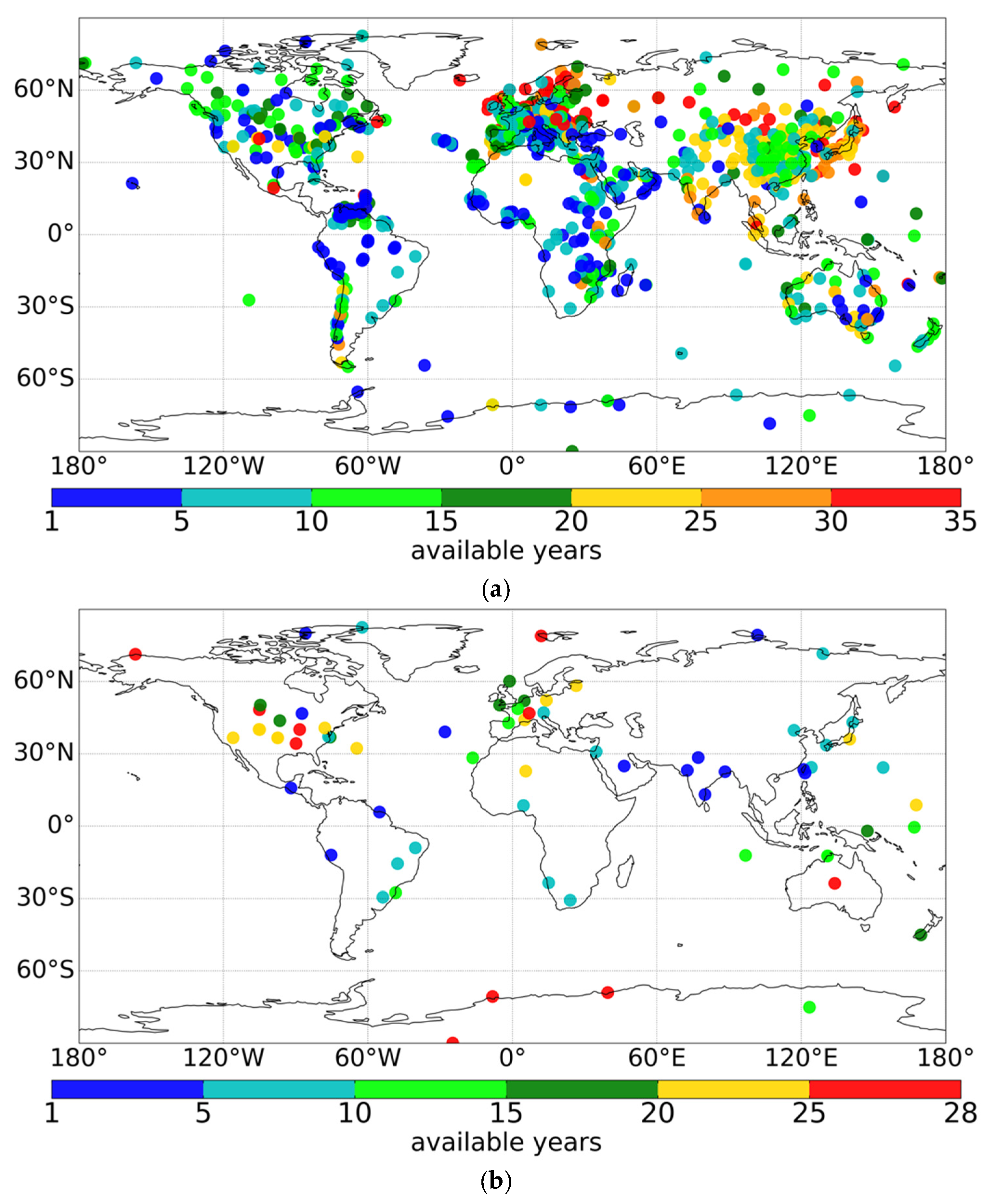
2.1.5. GEBA and BSRN
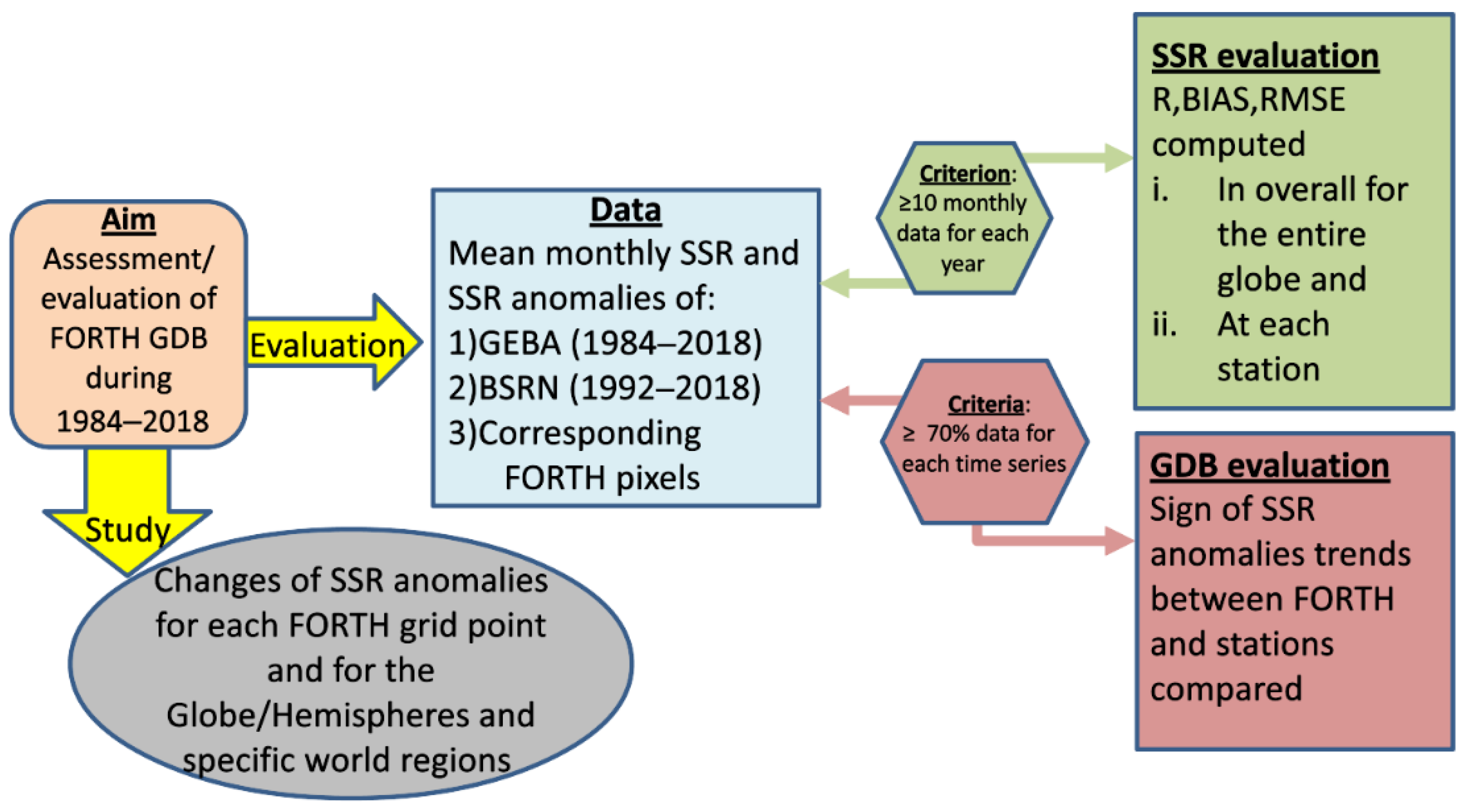
The GEBA network is maintained at the Institute for Climate and Atmospheric Sciences of the ETH (Zürich, Switzerland) and contains data from worldwide distributed ground-based measurements. It gives mean monthly values of 15 energy flux components, including surface albedo, longwave downward and upward radiation, and global, diffuse, and direct shortwave radiation, measured from 2500 globally distributed sites, with over 600,000 monthly values. Numerous stations offer measurements going back to the 1950s, and some even as far back as the 1930s. Their accuracy has been evaluated by [11] to be 5% of monthly means and 2% of annual means in terms of relative random measurement error. For the current study period 1984–2018, 1545 stations provided SSR monthly data, which were measured using pyranometers [60,61]. After registering at [62], users can use the GEBA data for free.
The World Climate Research Programme’s Radiation Panel project, the BSRN, is sponsored by GEWEX (WCRP). Since January 1992, it has been supplying high-quality radiation measurements with a high temporal resolution (one to three minutes) from 73 sites spread throughout different climate zones of the Earth. These measurements are sent to the Alfred Wegener Institute’s (AWI) BSRN Archive in Bremerhaven, Germany. SSR measurements from 73 BSRN sites for the years 1992 to 2018 are used in this study. Aside from the global shortwave flux (measured with pyranometers), the BSRN stations also measure the direct shortwave flux (measured with a pyrheliometer) and the diffuse shortwave flux (measured with a shaded pyranometer). The BSRN solar and thermal radiation data quality is described in detail in [63]. Under ideal observation conditions, an accuracy of up to 5 Wm−2 has been estimated using single pyranometers in conjunction with the component sum approach at BSRN locations [60]. This precision satisfies the BSRN standards. The daily data, which are derived from the instantaneous (minute level) data, are utilized to create the mean monthly BSRN data used for the evaluation of FORTH-RTM SSR and GDB. The BSRN data are available for free download at [64] via PANGEA or ftp. Figure S1 depicts the geographical distribution of the initially accessible GEBA and BSRN stations. These networks, especially GEBA, cover practically the entire globe (continental areas) with varying degrees of density (GEBA is denser than BSRN), while there is a dense GEBA network of stations in Europe and East Asia.

2.2. Methodology

The FORTH-RTM GDB was evaluated against GEBA and BSRN measurements using monthly mean SSR deseasonalized anomalies (created by subtracting the relevant long-term averaged value, which is different for each station, from each monthly SSR value) and fluxes. Since the use of deseasonalized anomalies reduces the seasonal component of temporal variability forced by the Earth’s orbital parameters, anomalies were preferred in the computation and evaluation of both the correlation coefficients and the trends of time series. Moreover, the absolute monthly SSR fluxes were used to compute/evaluate the other statistical metrics of FORTH-RTM SSR, including the absolute and relative percent bias and root mean squared error (RMSE). In order to assure the highest level of robustness for the resulting findings and conclusions, specific data availability criteria have been employed in the study. So, to avoid years with poor seasonal representation, which would worsen the comparison quality, each year’s fluxes were required to contain more than 10 monthly measurements. The application of this criterion resulted in the availability of 1193 GEBA and 66 BSRN stations (out of the originally available 1545 GEBA and 73 BSRN stations, respectively). These stations, which are seen in Figure 1, continue to provide sufficient geographic coverage of the world’s continents, albeit more so for GEBA than BSRN. Figure 2 depicts the steps of the applied methodology.
The Pearson’s correlation coefficient (R), Root Mean Squared Error (RMSE) and % relative RMSE (RRMSE), bias, and relative bias were used to measure the degree of agreement/disagreement between the FORTH-RTM model and reference stations’ SSR. Their respective equations are:
R = i = 1 n M i M G i G i = 1 n M i M 2 i = 1 n G i G 2
R M S E = 1 n i = 1 n M i G i 2
R R M S E = 1 n i = 1 n M i G i 2 G 100 %
B I A S = M G
B I A S % = M G G 100 %
where n is the number of monthly data, Mi and Gi are the FORTH-RTM model and ground-based stations’ respective monthly values (for the −i month), and M and G are their respective means. The RMSE (Equation (11)) measures the typical magnitude of the error, i.e., the typical difference between the FORTH-RTM and ground station values, whereas the R (Equation (10)) value measures how strongly the two variables correlate. The RMSE gives a relatively high weight to large errors because they are squared before being averaged; as a result, it is most helpful when large errors are particularly undesirable. The normalized relative percent RMSE is also computed in Equation (12). The bias (Equation (13)) quantifies the difference between the mean values of FORTH-RTM and observations. However, the relative percent bias (Equation (14)) is also used since it more accurately captures the difference, except for very small values. Linear regression is applied to the series of monthly deseasonalized SSR anomalies in order to assess the GDB, namely the change of SSR (Δ(SSR)) of both RTM and the measurements. The slope values were computed either for each station or the corresponding FORTH-RTM pixels, which include the stations. For the slope computation, we used a criterion for sufficient data availability, according to which, each time series should have an availability of more than 70% of the overall number of monthly values of the total period of each network. This allowed us to strengthen the confidence of the estimated slopes. This requirement was met by 22 BSRN stations and 222 GEBA stations (shown in the Supplement (Figure S2) as well as in the figures presented in Section 3, i.e., the Results). The Theil–Sen slope estimator [65,66], which is the median of all plausible linear slopes, was used to calculate the slope values because it is a more reliable nonparametric method. The computed slopes, which measure the changes per month, were multiplied by the temporal duration (in number of months) for each time series to produce the SSR changes Δ(SSR). The non-parametric Mann–Kendall Test [67,68], which is used to determine whether a time series has a monotonic upward or downward trend or not, was used to calculate the statistical significance of the slopes at a 95% confidence level. The slopes for each station were then compared with the slopes of the FORTH-RTM pixels that include the stations, to determine if they agree in terms of their signs of slope. For a given pixel, the qualitative agreement of the SSR changes (or GDB) between the FORTH-RTM and the GEBA/BSRN stations is indicated by the same signs of slopes of the FORTH-RTM and stations’ time series of SSR anomalies, whereas the opposite signs suggest a disagreement. This assessment is valuable because it measures how closely the FORTH-RTM GDB agrees, in signs, with the reference ground-based stations, quantifying the FORTH-RTM GDB confidence.

3. Results

3.1. Evaluation of FORTH SSR

Foremost, a thorough evaluation of FORTH-RTM SSR is carried out in this section, which is a requirement for the FORTH-RTM GDB evaluation. The evaluation is conducted either for all stations (Section 3.1.1) or on an individual station level (Section 3.1.2). The long-term (1984–2018) average of the FORTH-RTM SSR is shown in Figure 3, along with the corresponding long-term average SSR of GEBA and BSRN stations. The results reveal a generally nice agreement between the model and the ground truth SSR data.

3.1.1. All Stations

The statistics of the overall comparison of FORTH-RTM SSR fluxes and anomalies against 1193 GEBA and 66 BSRN measurement-based fluxes and anomalies are given in Table 1, while Figure 4 provides the corresponding scatterplot comparisons. It seems that FORTH-RTM SSR anomalies are satisfactorily correlated with GEBA and BSRN station anomalies yielding R values equal to 0.72 and 0.80, respectively (for the non-deseasonalized SSR fluxes the R values are much higher, as expected, equal to 0.96 for both GEBA and BSRN). Overall, the FORTH-RTM slightly underestimates SSR with respect to GEBA and BSRN, having negative mean biases equal to –4.71 and –14.29 Wm−2, respectively, corresponding to relative biases equal to –2.9% and –7.7%. The general underestimation of FORTH-RTM SSR against GEBA/BSRN may suggest that FORTH-RTM’s atmosphere is less transparent, which is consistent with other studies using the same model [7,8,30]. This could be the result of the overestimation of ISCCP cloud cover over the regions between 40° and 60° (where the majority of GEBA and BSRN stations occur) in both hemispheres as reported by [69]. They evaluated the ISCCP-H cloud cover against satellite data Cloud-Aerosol Lidar and Infrared Pathfinder Satellite Observation Cloud Product (CALIPSO-GOCCP) for 2000–2017 and their findings for Europe are in line (in terms of ISCCP overestimation) with those by [70] who validated ISCCP-H cloud cover over Europe against 22 meteorological ground-based stations from the European Climate Assessment & Dataset (ECA&D) for the period 1984–2012. Moreover, it seems that the aerosol input data do not contribute to the overall underestimation of FORTH-RTM SSR, since the MERRA-2 aerosol’s optical depth is in generally good agreement with observations as revealed by [71] who evaluated the MERRA-2 AOD against 468 AERONET stations globally for 1993–2016 and against 37 CARSNET (China Aerosol Remote Sensing Network) stations over China for 2002–2014. It should be noted that it has been reported in the literature [72] that the Chinese stations from GEBA, which count a significant number (103 stations), may not be as representative due to strong urbanization effects, so this can affect the comparison. In these stations, the FORTH-RTM overestimates the SSR by 2.66 Wm−2. Thus, excluding them from the comparison led to a stronger SSR overall underestimation equal to −5.45 Wm−2 (larger than the original by 15.7%). The estimated RMSE, which is equal to 21.02 Wm−2 for GEBA and 27.68 Wm−2 for BSRN (corresponding to 13.1% and 14.9% of the station networks’ mean values), shows that FORTH-RTM deviates slightly more from the BSRN and less from GEBA measurements. The slope values of the scatterplot comparison are 0.94 and 0.92, respectively, for GEBA and BSRN, while the corresponding values for SSR anomalies are equal to 0.68 and 0.82. It should be noted that in an assessment [8] of FORTH-RTM SSR, with a shorter period (1984–2000), lower spatial resolution (2.5° × 2.5°) and different input datasets (clouds from ISCCP-D2, aerosols from Global Aerosol Data Set, and meteorology from NCEP/NCAR global reanalysis data), the R values were equal to 0.99 for 700 GEBA and 22 BSRN stations, while the bias/RMSE values were equal to −6.49/23.44 Wm−2 for GEBA and –14/30.56 Wm−2 for BSRN), indicating again, similarly to the present work, that the model has larger underestimation and RMSE values against BSRN than GEBA stations. Moreover, the work by [30] and [7] used the FORTH-RTM for the period 2001–2006 and 2001–2009, respectively, with the same input data as [8] except for the aerosol data, which were taken from Moderate Resolution Imaging Spectroradiometer (MODIS)-Terra C005 and C006, respectively. The estimated SSR fluxes were validated against GEBA and BSRN stations and revealed similar performance to the work of [8] and the present study.
In addition to the FORTH-RTM SSR evaluation on an annual scale, this has also been carried out on a seasonal basis because this may help to more easily identify possible sources of errors. It should be noted that not only the absolute but also the relative biases were computed, because of the significant seasonal change of SSR fluxes. Table 1 shows that R using SSR anomalies and relative percent bias does not show significant seasonal changes, which are as large as 0.07 and 5.9%, respectively (the variability of relative bias is much smaller for GEBA, equal to 2.4%). Contrarily, BIAS and RMSE exhibit a discernible seasonal variation, up to 5.74 and 8.48 W/m2, respectively, with maximum values in NH (North Hemisphere) summer due to the highest absolute amounts of SSR, except over the BSRN sites where the highest BIAS occurs in NH winter. The relative RMSE also shows seasonal variations (up to 6.8/11.4% for GEBA/BSRN, respectively). Given the six-month shift in extreme seasons between the two hemispheres, the seasonal variation of the three main statistical metrics, namely R, RMSE (in absolute and percentage terms), and bias (in absolute and percentage terms) were also calculated separately for the two hemispheres and is shown in Figure 5. Except for R, which was calculated using deseasonalized SSR anomalies, the results of this figure were derived using SSR fluxes (the corresponding R using absolute SSR fluxes is given in Figure S3). Figure 5 shows that in general, the model correlates better with BSRN than GEBA, but it deviates more for BSRN than GEBA station measurements. Moreover, the statistical metrics do not exhibit a significant seasonal variation except for the absolute and relative values of BIAS and RMSE in the SH (South Hemisphere) for BSRN stations.

3.1.2. At Station Level

In order to examine if regional patterns exist in the metrics of the evaluation, it is necessary to study and compare the fluxes on an individual station basis as part of the evaluation of the FORTH-RTM SSR. The spatial distribution of the correlation coefficient (R) between the FORTH-RTM and GEBA/BSRN stations SSR anomalies is shown in Figure 6, along with the distribution of the RMSE, RRMSE, bias, and relative bias computed using SSR fluxes. For the GEBA stations, R ranges from –0.27 to 0.98, while for the BSRN stations, it ranges from 0 to 0.96. For 70% of GEBA/BSRN station data, the computed R values are greater than 0.62/0.67 (Figure S4). Satisfactory R values (orange and reddish colors) can be seen throughout Europe, East Asia, North America, and Australia. On the other hand, the tropical and subtropical world areas, such as Africa, South America, India, and Indonesia, tend to have worse R values (green colors and R smaller than 0.6). The same regional patterns, but with clearly higher values, appear for R computed using non-deseasonalized SSR fluxes (Figure S5). It can be assumed that the low correlation of FORTH-RTM SSR in these regions may be caused by uncertainties in cloud cover and optical properties, as also suggested by other studies [22,33,42], given that clouds are one of the primary factors driving the SSR [8]. Indeed, clouds are linked to the highest level of uncertainty in climate modeling [73,74], whereas the accuracy of ISCCP-H cloud cover is low over tropical and polar latitudes, as shown by [69] who evaluated the ISCCP–H cloud cover against the CALIPSO-GOCCP (GOCCP) during 2000–2017. Apart from clouds, however, aerosols can also contribute to the poor correlation in the tropics. An indication of this could be the low R values that can be observed in regions with little cloud cover, such as the Middle East and Egypt, which have high aerosol loads [53,75]. Polar locations also exhibit weak correlation, where the disparities may be brought on by issues with ISCCP clouds [76] as well as snow and ice cover [77,78]. In addition, southern China has lower R values than northern China (Figure 5 and Figure S5). Strong air pollution, as well as uncertainty in clouds, aerosols, and their interaction, might all be responsible for this pattern, as documented in previous research [22].
The difficulty of FORTH-RTM to accurately represent SSR in tropical and sub-tropical regions is confirmed by the large RMSE values observed in such areas over higher latitudes (Figure 6). Indeed, the range of RMSE values is 6.6–125 Wm−2 and 8.4–125 Wm−2, respectively, in the tropics and sub-tropics, while outside of them the corresponding ranges are 5.7–83.6 Wm−2. Similar regional patterns may also be observed for the relative RMSE, with high values being most prevalent across Southern China, polar regions, and some tropical and subtropical regions. In general, the FORTH-RTM underestimates SSR with respect to GEBA, overestimating it (yellow and red colors in Figure 6) over several tropical and subtropical areas, according to the results for the absolute and relative bias. This overestimation over low latitudes can be attributed to the underestimation of ISCCP-H cloud amount [69] and MERRA-2 aerosol loadings [79]. Overall, the model underestimates SSR fluxes in 832 stations, while overestimating it in 361 stations, yielding an underestimation of –4.71 Wm−2 for SSR fluxes on average. On the other hand, there is also an overall model underestimation of SSR fluxes by –14.29 Wm−2 when compared to the far fewer (66) BSRN sites (12 out of 66 overestimate). Absolute and relative percent bias range from –86.12 to 122.57 Wm−2 and from –41 to 92.7%, respectively. Yet, absolute and relative % bias values for 70% of the GEBA stations are less than 0.22 Wm−2/0.1%, respectively (Figure S4). At the BSRN sites, the relative % and absolute bias values range from –41.4 to 20.1% and –80.98 to 34.53 Wm−2, respectively, and 70% of the stations have relative and absolute bias less than –2.8%/−6.16 Wm−2, respectively. It should be noted that in the low latitudes, where the FORTH-RTM tends to overestimate the SSR fluxes, there are many more GEBA than BSRN stations, which can explain the weaker underestimation against GEBA than BSRN. Moreover, there are many sites that have a high mean bias over China, which is greater in its southern part, due to its incorrect assessment of cloud fraction and aerosol loadings [33,42,72,80,81].

3.2. FORTH-RTM GDB (SSR Trends) and Its Evaluation

After the detailed assessment of the FORTH-RTM SSR fluxes, which revealed quite a good performance, the FORTH-RTM SSR inter-decadal (1984–2018) changes (or GDB) are examined here. It should be emphasized that FORTH-RTM GDB has not yet undergone this examination over such a large time period (35 years), spatial distribution (0.5° × 0.625°), and use of state-of-art input data (ISCCP-H and MERRA-2). First, the GDB is evaluated either for the entire sample (all stations) or on a single-station basis (Section 3.2.1). Thereafter, Section 3.2.2 assesses and discusses the gridded FORTH-RTM GDB on a global and regional mean basis.

3.2.1. Evaluation of FORTH-RTM GDB (SSR Trends)

The GDB from the reference data of GEBA and BSRN stations was used to compare and evaluate the gridded FORTH-RTM GDB. By applying linear regression to the time series of monthly mean deseasonalized SSR anomalies, and then computing the slope values, the two sets of GDB, i.e., from the FORTH-RTM and the stations, were calculated. In order to ensure a high level of confidence for the results, this analysis was conducted for 222 (out of 1193) GEBA and 22 (out of 66) BSRN stations that satisfied the data availability criterion stated in Section 2.2 (more than 70% of the overall number of monthly values of the total period of each network. It should be mentioned here that the time period varies from station to station, ranging from 25 to 35 years for GEBA stations, and 19 to 27 years for BSRN stations, depending on the original temporal coverage of each station’s measurements and the applicable availability criterion (as shown in Figure S2, Supplementary). Each station’s time period was finally adjusted to the time period of the FORTH-RTM available data, i.e., 1984–2018.

All Stations

The comparison of the trends of SSR anomalies (in Wm−2) from the FORTH-RTM and GEBA/BSRN stations is shown in Figure 7 using a scatterplot. The correlation is poor, with average R values of 0.25 for GEBA and 0.32 for BSRN. Moreover, the slope values are low (0.11 for GEBA and 0.36 for BSRN) indicating that the model significantly underestimates the magnitude of GDB compared to stations. This is also demonstrated by the calculated biases (FORTH-RTM GDB—stations GDB), which are equivalent to –4.39/−4.59 Wm−2 for GEBA/BSRN. Likewise, the poor fit is revealed by the estimated RMSE values, which are equal to 11.95/7.67 Wm−2 for GEBA/BSRN. All these metrics prove that it is difficult for a model to reproduce the magnitude of the station GDB values. However, this is not extraordinary, since there are essential differences between the two sets of compared GDB, i.e., the modeled and measured ones, the most important one being that the model GDB refers to areas of 0.5° × 0.625° latitude x longitude, opposite to station GDB that pertain to specific sites.
Contrary to the magnitude of GDB, it is expected that it is more feasible for a model to reproduce the sign of GDB. This performance is easily assessed by the distribution of the Figure 7 scatterplot points to the four quartiles, with those lying in the first and third quartiles indicating the similarity of signs. There are 141 (115 in the first and 26 in the third quartiles) such data pairs for FORTH-RTM-GEBA (corresponding to 63.5% of the total number of points for the FORTH-RTM-GEBA scatterplot) and 12 (9 and 3 pairs) for FORTH-RTM-BSRN (corresponding to 54.5% of the total number of points for the FORTH-BSRN scatterplot), revealing that the FORTH-RTM reproduces partially satisfactorily the sign of stations GDB. Moreover, as for the performance of FORTH-RTM GDB, it was also assessed with respect to the altitude of stations, taking into account that the corresponding FORTH-RTM 0.5° × 0.625° grid cells’ mean altitude might not match the altitude of high-level stations. Most of the GEBA stations have altitude differences with their corresponding cells between 0–500 m. For such stations, as it concerns GEBA the agreement in the sign of the slopes is 66%, while for BSRN, it is 54.5% (note that all BSRN stations have altitude differences lower than 500 m). For the much fewer (6) GEBA stations that have altitude differences between 500–1000 m, there is agreement in 2 out of 6 stations and for those with differences larger than 1000 m, there is agreement only in 1 out of 4 stations. These findings indicate that the performance of the model decreases in the case of stations with high altitudes, but this does not significantly affect the overall model performance since the number of those stations is small.
Another aspect of the GDB comparison, apart from the overall scatterplot shown in Figure 7, is the overall performance of the RTM GDB, namely how the modeled GDB compares to that of stations on the average, as well as how the temporally varying averaged SSR anomalies match those of stations. In this aspect, the computed 12-month moving averages of SSR anomalies of all stations and the corresponding FORTH-RTM pixels over the total period for each network, i.e., 1984–2018 for GEBA and 1992–2018 for BSRN, are shown in Figure 8. Along with the 12-month moving averages, the number of stations that were accessible in each month/year is also shown. Since FORTH-RTM consistently shows larger/smaller positive SSR anomalies than GEBA before/after the year 2000, this results in low slope values and small average biases (FORTH-RTM—stations) equal to −0.072 and 0.064 Wm−2 against GEBA and BSRN stations, respectively. In association with the smaller slope values, weaker GDB is estimated by the RTM than for stations. Specifically, using the non-parametric Mann–Kendall test, GEBA stations (Figure 8a) suggest a statistically significant brightening, or positive Δ(SSR), equal to 5.82 Wm−2 as opposed to a lesser not statistically significant, brightening computed using FORTH-RTM (Δ(SSR) = 0.26 Wm−2). Comparable conclusions are reached from a similar analysis of FORTH-RTM and BSRN (Figure 8b). Indeed, a statistically significant brightening (Δ(SSR) = 5.31 Wm−2) is computed compared to a small, but not statistically significant, brightening of FORTH-RTM equal to 0.17 Wm−2. It is interesting to note that both GEBA and BSRN suggest a comparable brightening and that FORTH-RTM is, at least, able to reproduce the same sign of Δ(SSR) against both station networks. Here, it is also examined to what extent the number of stations, which changes with time, affects the differences between the 12-month moving average time series of stations and FORTH-RTM SSR. With respect to the GEBA stations, their number decreases after 2008, but this does not seem to have an effect on the differences. On the other hand, regarding the much fewer BSRN stations, the few available stations till 1999 produce larger differences on the time series than after 1999 when the stations availability increased.

At Station Level

Figure 9 shows the GDB for the GEBA/BSRN stations (the time period varies for each station) and the FORTH-RTM pixels that contain these stations. These findings make it possible to evaluate the GDB produced from the model and stations and to compare them in terms of the sign and magnitude of either GDBs. In addition to the calculated trends, the results of the non-parametric Mann–Kendall test, which has been applied to estimate their statistical significance at the 95% level, are also shown in Figure 9. Mostly positive and statistically significant trends over Europe and East Asia are revealed by the stations, especially GEBA and GDB, in contrast to mainly negative and statistically significant trends over India. The positive and negative trends for GEBA stations range from 0 to 33.81 Wm−2 and from −0.38 to –37.91 Wm−2 whereas the respective ranges for BSRN stations are 0.92–13.55 and −(0.7–6.24) Wm−2. It should be noticed that irrespective of their sign, statistically significant trends are identified for 161 out of 222 (or 72.5%) GEBA and 11 out of the 22 (50%) BSRN stations. The 222 GEBA stations that have been used show an average brightening of 5.00 Wm−2, compared to 3.58 Wm−2 (brightening as well) for the 22 BSRN stations.
While the corresponding ranges of GDB for the FORTH-RTM pixels that include the BSRN stations are 0.30–9.99 and −(0.99–13.7) Wm−2, the obtained trends of GDB for FORTH-RTM pixels including the GEBA stations show larger positive trends, ranging from 0.06 to 14.88 Wm−2, and negative trends from 0.01 to 20.23 Wm−2. The positive and negative ranges of GEBA GDB are both larger than the corresponding FORTH-RTM ranges, whereas the positive/negative ranges of BSRN GDB are larger/much smaller than the FORTH-RTM corresponding pixels. Based on the results of Figure 9(i-b,ii-b), the average GDB of the FORTH-RTM pixels including the GEBA sites is a brightening of 0.61 Wm−2, which is smaller than the 5.00 Wm−2 equivalent brightening of GEBA sites, while the average GDB of the FORTH-RTM pixels including the BSRN sites is a dimming of −1.01 Wm−2, opposite to the brightening of 3.58 Wm−2 for the BSRN stations. Irrespective of their sign, statistically significant trends are identified for 56 out of 222 FORTH-RTM pixels including GEBA stations (i.e., for 25.2%) and for 8 out of the 22 (36.6%) pixels containing BSRN stations. Moreover, the same findings, namely agreement/disagreement in the sign of GDB between the FORTH-RTM and GEBA/BSRN stations, are found if only pixels with either model and stations with statistically significant GDBs are used. The mean GDB for GEBA/BSRN sites is 6.41 and 5.79 Wm−2, whereas the average FORTH-RTM GDB for GEBA/BSRN sites is 0.32 and –4.45 Wm−2. Moreover, strong and statistically significant dimming over India and strong brightening over Europe are both shown by FORTH-RTM pixels and GEBA stations but with GEBA stations showing a stronger brightening than FORTH-RTM. On the other hand, there are other regions such as Korea and China where there is disagreement, with the RTM showing a dimming against the brightening indicated by the stations. This disagreement also occurred in the comparison of MERRA-2 and GEBA GDB made by [41], suggesting that this disagreement could be attributed to possible problems in the common input aerosol data (from MERRA-2). According to our analysis, this dimming in our model primarily arises from increasing MERRA-2 aerosol loadings. This increase, which continues during the period 2001–2016 as also revealed by [71] in mainland East Asia, is in strong disagreement with the MODIS/Terra and MISR observations. However, on the other hand, there are issues in GEBA stations associated with the strong urbanization effects [72] which can also explain the disagreement in SSR changes between FORTH-RTM and GEBA stations in Korea and China.
The agreement or disagreement between the signs of GDB estimated (using SSR anomalies) by either the FORTH model or the GEBA/BSRN stations is clearly shown in Figure 10. The signs of FORTH-RTM and GEBA GDBs show a satisfactory percentage of the overall agreement (63.5%), whereas the percentage for the much fewer BSRN stations is lower (54.5%). Furthermore, it is found that for cases (pixels) with statistically significant trends, the percentage of agreement is higher for GEBA, equaling 76.7%, and lower, equal to 50%, for BSRN stations (which are however only 4). The obtained results from the analysis utilizing GEBA stations, which offer a fair amount of geographical coverage throughout continents like Europe, India, or Australia, allow the inference of confident conclusions about a fairly systematic agreement over these world regions. Thus, it is found that most stations (66.4%) in Europe exhibit qualitative agreement (same sign for GDB). Additionally, there is a complete agreement over India, extraordinarily for all GEBA stations. Moreover, almost all stations over Australia (80%) and most stations in Japan (73.1%) show an agreement as well. In North America, a mixed pattern exists with agreement/disagreement in 5/5 (i.e., 50/50%) BSRN stations. It is interesting to note that while in the current analysis, using the values of the 22 chosen BSRN stations, agreement in the sign of GDB is found at 54.5% of stations, when the total number of BSRN stations (66) is used, without applying the availability criterion in the computation of SSR trends, agreement is found at more stations, i.e., 66.7% of stations. On the other hand, for the entire group of GEBA stations (1193), an agreement of 66% is found, just slightly higher than 63.5% for the selected 222 stations. The results of the present study are comparable to those obtained with similar versions of the same model (FORTH-RTM), but using somewhat different input datasets and referring to much shorter time periods, i.e., 2001–2009 in [7] and 2001–2006 in [30] and numbers of GEBA/BSRN stations (105/20 in [7] and 91/14 in [30]), suggesting that the FORTH-RTM GDB has a good qualitative agreement with GEBA stations (for more than 60%) and a poorer, but still reasonable, agreement against the much smaller sample of BSRN stations, which is greatly affected by the number of available stations and it is larger than 54.5%. In a recent study, Ref. [41] estimated the MERRA-2 GDB and the degree of its agreement with GEBA and BSRN stations almost for the same time period (1980–2019) as the present study. They reported that the MERRA-2 GDB agrees for 63.4% GEBA and 50% BSRN stations, indicating that the degrees of FORTH-RTM and MERRA-2 GDB agreement with the GEBA/BSRN reference stations are comparable, suggesting possible issues in the common input data from MERRA-2.
SSR strongly depends on solar radiation absorbed and reflected in the overlying atmosphere at every location. Thus, an additional analysis was conducted to examine if the FORTH-RTM fluxes successfully represent the closure of the solar radiation budget with the aim of more fully assessing the robustness of the modeled GDB. To achieve this, specific GEBA/BSRN stations that offer GDB agreement with the model were initially chosen. Then, the computed trends of the FORTH-RTM Outgoing Solar Radiation (OSR) at TOA for these stations were compared to the matching OSR from CERES-EBAF satellite data for the time period 01/2001–12/2018 to investigate if they agree or disagree in terms of the sign of Δ(OSR). For those sites where both the modeled Δ(SSR) and Δ(OSR) qualitatively agree with the corresponding reference surface and satellite measurements, the Earth’s SW radiation budget is successfully closed. It should be noted that in this case, the available number of stations is 256 for GEBA and 32 for BSRN based on the criterion according to which each station should have availability of more than 70% of the number of months for the entire time period (2001–2018). It should be noted that, during this period, the MERRA-2 products assimilated modern satellite data, leading to a more homogenous time series [53] for the FORTH-RTM aerosol input data. In this case, with a shorter time period than previously (1984–2018), the level of agreement between the sign of slopes of stations and FORTH-RTM pixels slightly improved for GEBA and hardly decreased for BSRN. Figure 11 compares the signs of the computed FORTH-RTM Δ(SSR) and Δ(OSR) with the equivalent GEBA/BSRN Δ(SSR) and CERES-EBAF Δ(OSR) signs. At the surface, 67.6% of GEBA (173 out of 256) stations and 53.1% of BSRN (17 out of 32) stations agree with FORTH-RTM in terms of Δ(SSR) sign (blue dots in Figure 11(i-a,ii-a), respectively). Then, just for those stations (providing agreement on the surface), the signs of Δ(OSR) from FORTH-RTM and CERES were compared. Out of the 173 GEBA sites, there was qualitative agreement at TOA for 145 stations, i.e., in 83.8% of them. Accordingly, an agreement was observed for 88.2% of the 17 BSRN locations, which is almost equal to the percentage for GEBA. Overall, 145/15 (56.6/46.9%) of GEBA/BSRN stations provided agreement in the sign of both Δ(SSR) and Δ(OSR). The obtained results of this part of the analysis, focusing on the comparison between the changing solar fluxes at the Earth’s surface and TOA as estimated with the FORTH-RTM against reference surface and TOA fluxes, prove that FORTH-RTM partially satisfactorily reproduces the changing SW radiation budget and especially GDB.
Since GDB experiences variations on a decadal scale, as described in Section 1, the agreement/disagreement between the FORTH-RTM and stations’ GDB has also been evaluated across certain sub-periods. According to the literature [6,17] based on station measurements, the chosen sub-periods and the accompanying GDB patterns are 1984–1989 (dimming), 1990–1999 (brightening), 2000–2009 (reduced brightening), and 2010–2018 (brightening and dimming). For each sub-period, time series of deseasonalized FORTH-RTM and station SSR anomalies were produced, a linear regression was applied to them, and Sen’s slope was computed. The results are shown at a station level in Figure S6, whereas Table 2 and Table 3 for GEBA and BSRN, respectively, emphasize the agreement or disagreement between the sign of the computed average GDB from all stations and the corresponding FORTH-RTM pixels. According to Table 2, 66.1% of GEBA stations during the 1980s had a qualitative agreement with the FORTH-RTM in terms of the GDB sign, compared to 60% during 1990–1999, 51.2% during the 2000 to 2009 period, and 73.2% for 2010–2018. The higher level of agreement during the first, second, and fourth periods is in line with (or results in) the identical sign of overall (averaged) GDBs from the model and GEBA stations, consisting of dimming in 1984–1989 and brightening in 1990–1999 and 2010–2018. Regarding the comparison against BSRN stations (Table 3), agreement is found for 63.6% of stations from 1992 to 1999, 50% from 2000 to 2009, and 65.9% from 2010 to 2018. Again, during the first (1990s) and third (2010s) periods, the higher percent number of stations with agreement, resulted in the same sign of GDB (brightening in both periods) as estimated from the model and BSRN stations. It is also noticeable that during the 1980s, 1990s, and 2010s, the FORTH-RTM qualitatively reproduces the GDB indicated by both reference GEBA and BSRN station networks, exhibiting good performance. Only in the 2000s, the sign of the modeled GDB is the opposite of the one suggested by stations, namely a modeled dimming against station-based brightening. With respect to the magnitude of model GDB, it not necessarily follows the interdecadal changes suggested by the GEBA and BSRN stations (for example the GEBA brightening in the 2010s is about 1.3 times stronger than that in the 1990s, while the corresponding modeled one is 1.9 times, whereas the corresponding 2010s/1990s GDB ratios for BSRN stations are 0.07 for BSRN and 1.4 for FORTH-RTM), but this is of secondary importance compared to the similarity/dissimilarity of the estimated GDB itself.

3.2.2. The FORTH-RTM GDB on Global, Hemispherical and Regional Scales

The global distribution of the FORTH-RTM GDB, or Δ(SSR), during the 35-year period from 1984 to 2018, is shown in Figure 12. The calculated Δ(SSR) values came from applying linear regression to the time series of deseasonalized monthly FORTH-RTM SSR anomalies for each pixel and computing the Sen’s slope. The same figure also contains information about the statistically significant GDB (dotted pixels). Over southern and eastern Europe, the Middle East, the Central African Republic, western North Africa, Mexico, and the southern USA, several areas of the Tropical and sub-tropical oceans, as well as Brazil and Argentina, strong and statistically significant brightening (up to 100.49 Wm−2 or 2.87 Wm−2 year−1) is observed, according to FORTH-RTM. On the other hand, strong and statistically significant dimming, as large as –46.2 Wm−2 or −1.32 Wm−2 year−1, is observed across the western Tropical Pacific, India, Mainland Southeast Asia, East China, Indonesia, Guinea Gulf, and offshore SW Africa, western Australia, Siberia, northern South America and several remote oceanic regions, including the Southern and Arctic Ocean. Over many regions including large parts of North America, central Europe, Russia, eastern Australia, and the Eastern Sahara, no statistically significant trends were computed. In nearby regions over extended world areas including Africa, North and South America, Australia, the eastern Tropical Pacific, and the Eastern Mediterranean, SSR trends are opposite. Dimming is found in 53.7% of pixels, against 46.3% showing brightening, leading to an overall global dimming equivalent to 2.2 Wm−2. In 50% of pixels globally, the SSR changes are statistically significant, according to our findings. In those cells with statistically significant GDB, solar dimming dominates even more, occurring in 63% of them. While brightening somewhat predominates over land (brightening/dimming occurring in 54.7%/45.3% of pixels), a dimming is observed over oceans (brightening/dimming in 42.1%/57.9% of pixels) explaining the overall global dimming. The identified SSR changes are attributed to the changes in the model input data that are relevant for SSR, namely cloud cover, cloud optical thickness, aerosol optical depth, and water vapor. The global distribution of these changes during the study period (1984–2018), are shown in Figure S8. According to them, it seems that the decreasing SSR trends over India, Guinea Gulf, Indonesia, N. South America and East Asia, are caused by the statistically significant increasing trends of AOD, cloud optical thickness, and water vapor (cloud cover showing either decreasing or weak increasing trends over these regions). On the other hand, the brightening over Europe arises from the decreasing AOD and cloud cover whereas cloud optical thickness and water vapor show increasing trends. Moreover, the solar dimming observed over Australia is found to arise from increasing trends of water vapor and cloud cover. These findings indicate that the main causes of GDB are different from one world region to another, which underlines the complexity of the phenomenon. It is noticeable that some similar patterns of brightening (over Europe, Mexico, Central Africa, and parts of tropical oceanic regions) and dimming (over India, Australia, Northern South America, Guinea Gulf, and Indonesia) were revealed by the work of [41] during almost the same time period of 1980–2019 and using the MERRA-2 SSR product. Seasonal change of GDB features on a regional level is revealed by additional information about the FORTH-RTM GDB derived on a seasonal basis (Figure S7). For instance, the annual brightening seen over Europe (Figure 12) is driven by substantial brightening in boreal spring, namely the months of March, April, May, and in boreal summer (June, July, August) while dimming is observed therein during autumn (September, October, November) and winter (December, January, February). Moreover, the annual dimming over Siberia arises mainly from dimming in boreal summer months, while the dimming over Australia is stronger in boreal winter and over Northern S. America in boreal spring. A stronger dimming is seen in the months of June through November over East China and December through March over SE Asia, causing the respective annual mean dimming patterns. A systematic dimming is seen throughout the year across the Southern Ocean, being stronger in boreal winter and spring months, the Pacific Tropical Warm Pool, and India, culminating in an annual dimming over these regions. Additionally, the annual dimming over the Sahara (Figure 12) results from a dimming that occurs mainly during boreal summer and secondarily boreal autumn. It should be mentioned that the artificial patterns of GDB that can be observed in Figure 12 are introduced by the artifacts on ISCCP-H cloud data, which are linked with changes in satellite viewing geometries [82,83,84,85]. More specifically, there are relevant patterns centered in the Atlantic, Indian, Western Pacific, and Eastern Pacific Oceans which correspond to the geostationary “footprints” that describe the area observed by each satellite. At the edge of these footprints, the satellite’s zenith angle is much higher, corresponding to a longer path length through the atmosphere that light must travel before it is detected by the sensor. For instance, the pattern over the Indian Ocean is connected to the area where geostationary data were not available until 1997, and AVHRR polar-orbiting satellite data were used instead [83], while the pattern in the Atlantic Ocean is linked to the actual coverage from the geostationary satellite METEOSAT [86]. However, these artificial patterns occur mostly over ocean areas, and thus could not be validated against ground truth measurements. Yet, on the contrary, they are absent over land areas, thus providing confidence about the reliability of the FORTH-RTM GDB at least in qualitative terms, as demonstrated by the evaluation performed in the previous section.
The time series of the calculated average deseasonalized SSR anomalies for the Globe, the northern hemisphere (NH), and the southern hemisphere (SH) over the 35-year period from January 1984 to December 2018 is shown in Figure 13, providing an easy assessment of the interdecadal patterns of global and hemispherical GDB. The FORTH-RTM global mean SSR anomalies vary up to 16.86 Wm−2 (from −7.33 to 9.53 Wm−2), while the northern/southern hemispherical SSR anomalies range from −10.23/−9.36 to 7.49/16.46 Wm−2, respectively. The applied 4th-order polynomial fit to the global 35-year time series indicates that between 1984 and 1989 a decreasing SSR tendency occurred over the Globe, which reversed to a brightening in the 1990s and till 2000. Subsequently, a dimming took place in the first decade of the 21st century, followed by a brightening in the last decade, i.e., in the 2010s. This results in an overall negative trend (dimming) during the entire 1984–2018 period, either globally or in both hemispheres. Note that globally, according to Figure S9, which shows the interannual and interdecadal variability of mean annual SSR fluxes and 4 basic model input data, the solar dimming during 1984–1989 is primarily due to increasing cloud optical thickness, while the brightening in the 1990s is attributed to decreasing cloud optical thickness, cloud cover, and AOD. Moreover, it is found that the global dimming during 2000–2009 is caused mainly by the increasing cloud optical thickness and AOD, while the brightening in the 2010s is attributed to cloud cover, optical thickness, and AOD. These results highlight that the GDB is not only driven by different factors over different world areas, but that even for a given area the factors can be different from one decade to another, thus further perplexing the phenomenon. Yet, at least globally, cloud optical thickness overall clearly dominates the SSR variations (except for the Pinatubo signal at the beginning of the 1990s), both in terms of inter-annual variations (e.g., strong peak in 1994 explained by cloud optical thickness low peak) as well as the longer term variations (polynomials of SSR and cloud optical thickness fit very well), and even in the overall trend. Between 1984 and 1995, the SH (red line in Figure 13) experienced stronger positive anomalies than the NH (green line), whereas afterward, the SH experienced larger positive anomalies than the NH until 2018 (the opposite inter-hemispherical predominance exists for the negative SSR anomalies). Most existing measurements-based and modeling studies agree with the increase in SSR suggested by FORTH-RTM during the years from 1990 to 2000 [8,12,13,16], while the negative trend for the years 2000 to 2009 is also consistent with other studies [7,30,32]. Strong SSR decreases brought on by the large volcanic eruption of Pinatubo (1991), as well as by strong El-Nino phases (1997, 2002, 2009, or 2016), are reproduced by FORTH-RTM. Years that were affected by the recovery from Pinatubo, as well as the La-Nina phases (1989, 1999, or 2006), are distinguished by positive anomalies. These results demonstrate that the FORTH-RTM satisfactorily reproduces natural processes that affect Earth’s radiation budget and climate, such as volcanic eruptions and the ENSO (El Nino Southern Oscillation). Note, that a similar analysis to that shown in Figure 13 was performed by [41] using the MERRA-2 SSR, which did not reveal the brightening phases in the 1990s or in the 2010s, although both MERRA-2 SSR and FORTH-RTM SSR were computed with the same aerosol information. This underlines how the different cloud data (ISCCP-H observations vs. MERRA-2 calculated clouds) impact the estimated GDB.
The FORTH-RTM has the advantage of covering a quite long 35-year (climatological) time period that includes strong anthropogenic global warming (starting from the ‘80s). There have been theories and studies on how GDB interacts with the current rapid global warming, either accelerating or counteracting it [4,10,14,87,88], most of which are based on surface station data of SSR. Hence, the FORTH-RTM-based determination of GDB at vast geographical (global) and temporal (35-year) scales allows for a better assessment and comprehension of the contribution of GDB to global warming, in connection to the dominant role of anthropogenic greenhouse gases. To do this, the four sub-periods which were previously defined were selected as characterized by different phases of GDB. The results computed on a worldwide and hemispherical scale, as well as separately for land and ocean areas, are shown in Table 4. According to the FORTH-RTM, the overall Δ(SSR) during the period 1984–2018 is equal to −2.22 Wm−2 or −0.063 Wm−2 year−1 on a global scale (dimming), with dimming being detected in both hemispheres (−0.48 and −2.73 Wm−2 or 0.014 Wm−2 year−1 and −0.078 Wm−2 year−1, being stronger over SH. Note that the aforementioned Δ(SSR) changes are all statistically significant at a 95% confidence level (CL). Oceans show a stronger dimming (−2.56 Wm−2 or −0.073 Wm−2 year−1, statistically significant at 95% CL) than land (−1.04 Wm−2 or 0.03 Wm−2 year−1, not statistically significant), which is consistent with the stronger global warming (+0.32 °C decade−1 and +0.14 °C decade−1, [89]) recorded over land than oceans. The two hemispherical land and oceanic regions, and thus the two hemispheres and the globe, have the same sign of GDB for each time sub-period. Specifically, over the globe, the two hemispheres, and the NH and SH land and ocean areas, solar dimming occurred between 1984 and 1989, followed by a stronger brightening between 1990 and 1999, which is consistent with the accelerated greenhouse global warming after 1980 [90,91]. Then, during the first decade of the 21st century, a decreasing SSR trend (dimming) took place over the globe, the two hemispheres, and the land and ocean areas of both NH and SH, which is in line with the hiatus of the global warming during this decade [91,92,93]. Then the tendency shifted into an increasing SSR trend (brightening) between 2010 and 2018, which is compatible with the recent acceleration of global warming [91,94].
Given that GDB is a regional phenomenon (Figure 12), a regional study was carried out to identify decadal scale GDB features. To achieve this, three distinct regions of the globe were chosen, (Europe’s, Japan’s, and India’s land areas, shown within the rectangles in Figure 12), each of which has adequate station coverage and displays homogeneous GDB patterns (Figure 12). For each selected area, three time series of deseasonalized SSR anomalies (for the period January 1984–December 2018) were created, one for the region’s GEBA stations (122 sites in Europe, 18 in Japan, and 7 in India) that meet the slope estimation criterion as stated in Section 2.2, a second time series for the corresponding FORTH-RTM pixels including the GEBA stations and a third for all of the FORTH-RTM pixels within the geographical limits of the region. The time series are provided in Figure 14 together with their applied linear regression, while the polynomial 4-th order fit applied to the third (all model pixels) time series is also plotted. This analysis enables us to assess the ability of the FORTH-RTM GDB to reproduce the GDB measured at the sites of GEBA stations within each region. In general, it is revealed that FORTH-RTM satisfactorily represents the month-to-month and year-to-year variability of SSR (correlation coefficients equal to 0.61, 0.70, and 0.59, respectively, for Europe, Japan, and India). For India, we compute a strong dimming for the GEBA measurements (−32.15 Wm−2) against a smaller dimming for the corresponding model pixels (−9.58 Wm−2) and for the total land of India (dimming equal to −6.72 Wm−2). This much stronger dimming for GEBA is associated with a much larger/lower GEBA than model positive/negative anomalies before/after 1994/2010. In contrast, over Japan, a brightening equal to 10.41 Wm−2 occurred according to GEBA station measurements, stronger than a marginal brightening of 0.36 for the FORTH-RTM pixels and 0.86 for the total land of Japan. Regarding the European land areas, a brightening during the entire time period is computed, which is stronger for GEBA stations (9.13 Wm−2) than the corresponding FORTH-RTM land pixels (3.29 Wm−2) and all Europe’s land pixels (3.56 Wm−2). Over Europe, the brightening in the 1990s is followed by dimming in the 2000s and then by a brightening again after 2010. It should be noted that the dimming in the 2000s and the consequent brightening is also found over Japan and the Indian subcontinent. Our findings demonstrate the FORTH-RTM’s capacity to qualitatively represent the GDB (dimming or brightening) observed at GEBA stations over the continental regions of Europe, Japan, and India. The obtained results of Figure 14 show that, in line with other studies ([14] and references therein), there was a brightening over Europe (land) from 1984 to 2000. According to our results, this brightening reversed to a weak dimming after 2000, which is relatively similar to the tendency of SSR stabilization since the early 21st century suggested by [95]. Agreement is also found with the limited available literature for India, according to which [96] a dimming was observed over India during 1981–2004, based on 12 ground-based stations while the study by [97] also based on 12 ground-based Indian stations, estimated a level-off of the dimming in the late 2000s over most stations. On the other hand, according to [98], who used 14 ground-based meteorological Japanese stations, there has been a dimming during the 1980s, which reversed to a brightening phase in the 1990s in line with our results.

4. Conclusions

Satellite observations along with radiative transfer model computations are advantageous in that they offer worldwide coverage and long-term data for the important climate parameter of SSR and its long-term tendencies (GDB). Inaccuracies in the input datasets to the models, however, could result in errors in SSR and its interannual variability and trends and, consequently, inaccuracies in research using them, e.g., estimated GDB. Therefore, it is essential to evaluate SSR products against reference ground measurements prior to their use in climate research. Here, for the first time to our knowledge, a detailed evaluation of the FORTH-RTM SSR fluxes and SSR interdecadal changes is attempted, against high-quality ground-based measurements from 1193 GEBA and 66 BSRN stations, on a global, regional, and station level, for the 35-year period 1984–2018. The following is a summary of the key findings from the analysis that was carried out.
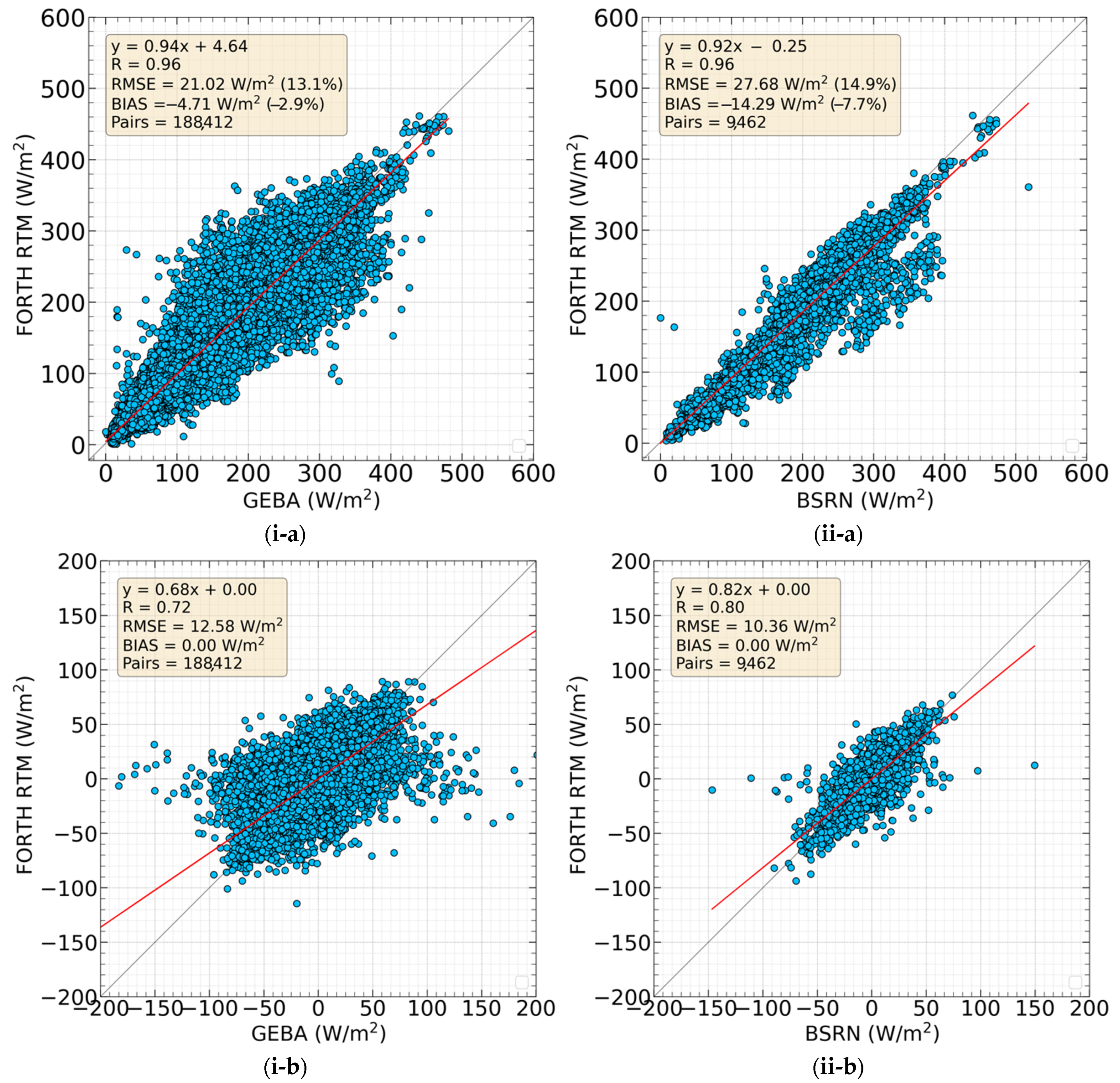
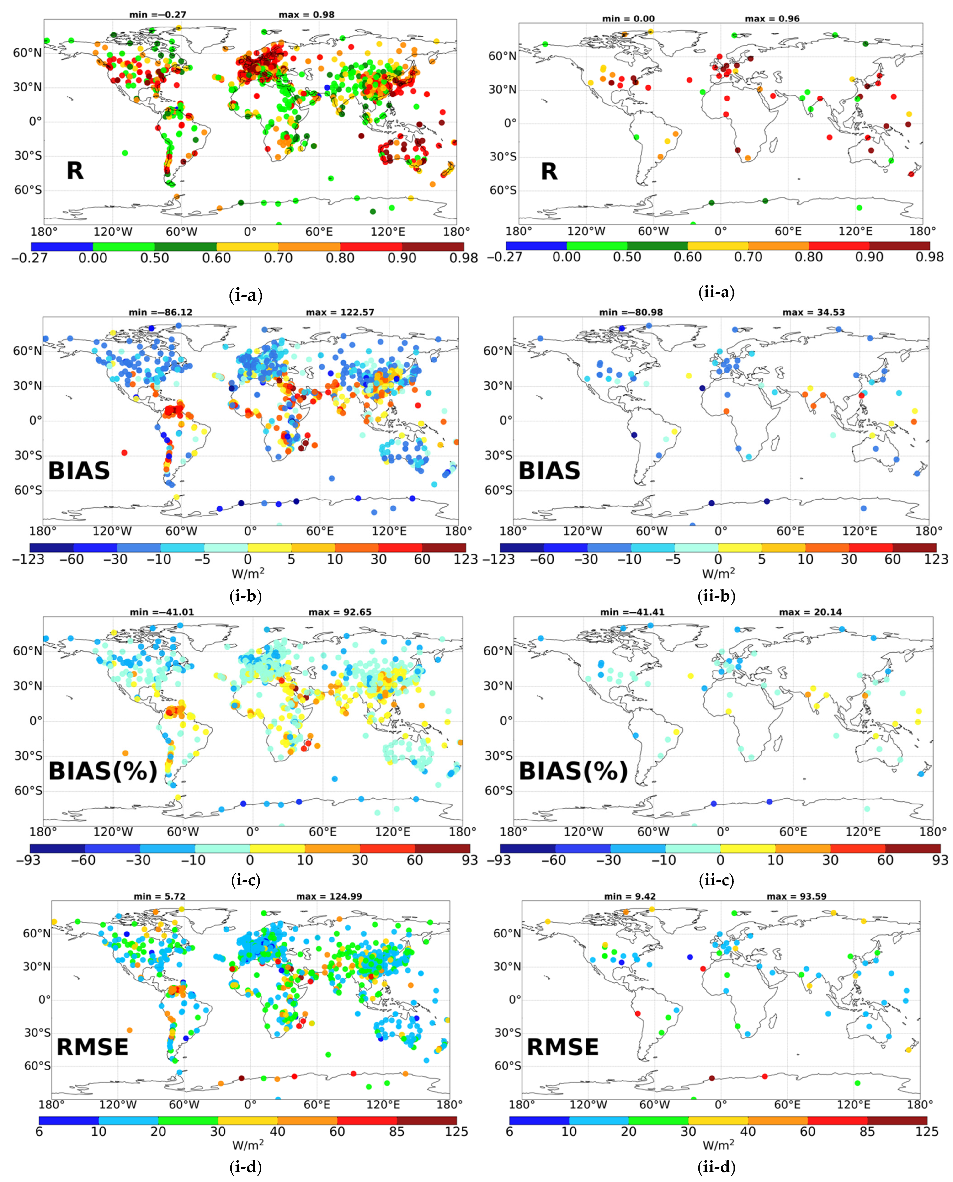
  • The FORTH-RTM deseasonalized SSR anomalies, which are free of the seasonal cycle, correlate very well with the ground-based measurements, with R values equal to 0.72 and 0.80 for the validation against GEBA and BSRN stations, respectively. On a station level, the computed R values range from −0.27 to 0.98, but the majority of them (61%) are higher than 0.7, with the lowest values occurring in low latitudes, possibly due to uncertainties in the cloud and aerosol input data.
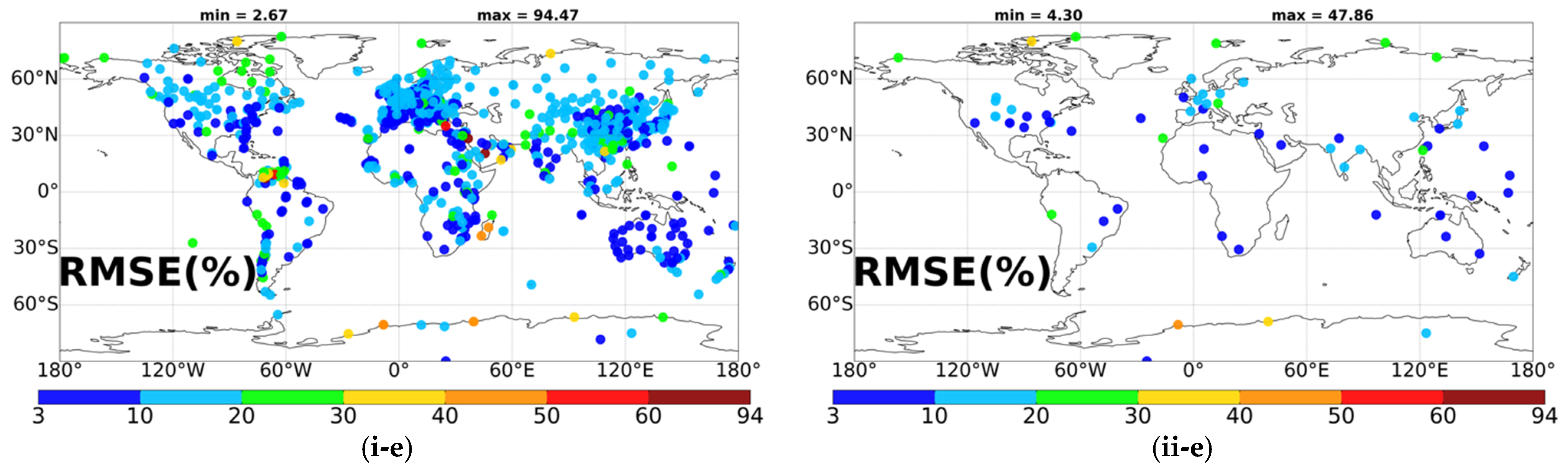
  • In general, there is a relatively small underestimation of FORTH-RTM SSR compared to GEBA and BSRN measurements, the mean bias being equal to −4.71 Wm−2 and −14.29 Wm−2 or −2.9% and −7.7%, respectively. However, FORTH-RTM overestimates SSR at low latitudes, probably because of an underestimation of cloud cover and aerosol optical depth data in these regions. The general underestimation suggests that the atmosphere of FORTH-RTM is less transparent than it should be. The average RMSE value is equal to 21.02 Wm−2 (equivalent to 13.1%) for the comparison of FORTH-RTM with GEBA, while the corresponding value for BSRN is equal to 27.68 Wm−2 or 14.9%, pointing to a rather small deviation of the modeled from the measured SSR. The largest RMSE values exist in low and high-latitude regions.
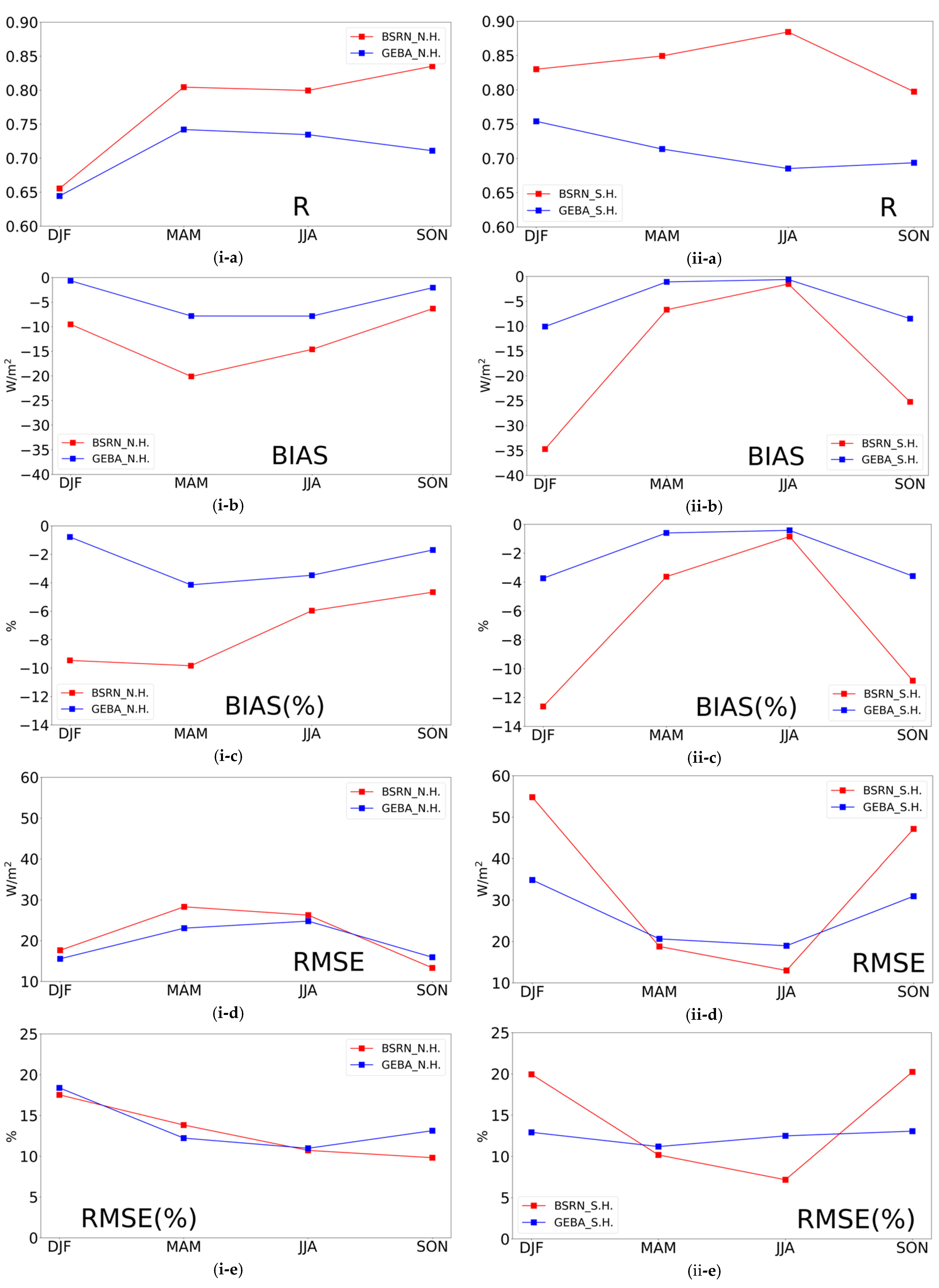
  • In all seasons, the model performs better in terms of R, but worse in terms of deviation, with BSRN than GEBA station measurements. Moreover, the evaluation metrics do not exhibit a significant seasonal variation except for BIAS and RMSE in the SH for BSRN stations.
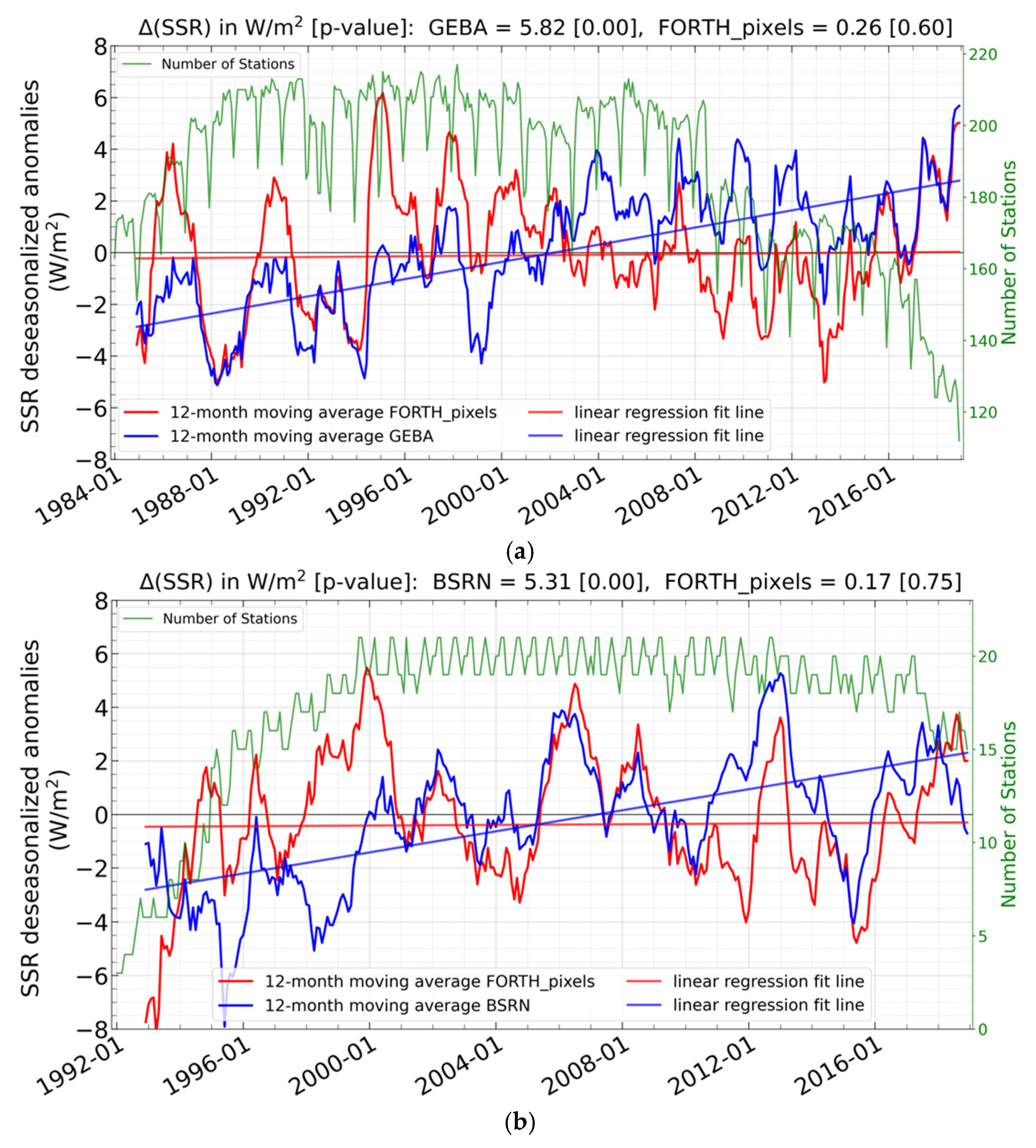
  • The comparison of the time series of 12-month moving averages between FORTH-RTM SSR anomalies and GEBA/BSRN sites shows a larger model than station SSR anomalies, positive before 2000 and negative after 2000, which can affect the computed GDB. Indeed, the FORTH-RTM SSR trends show a weaker brightening than the stations’ trends.
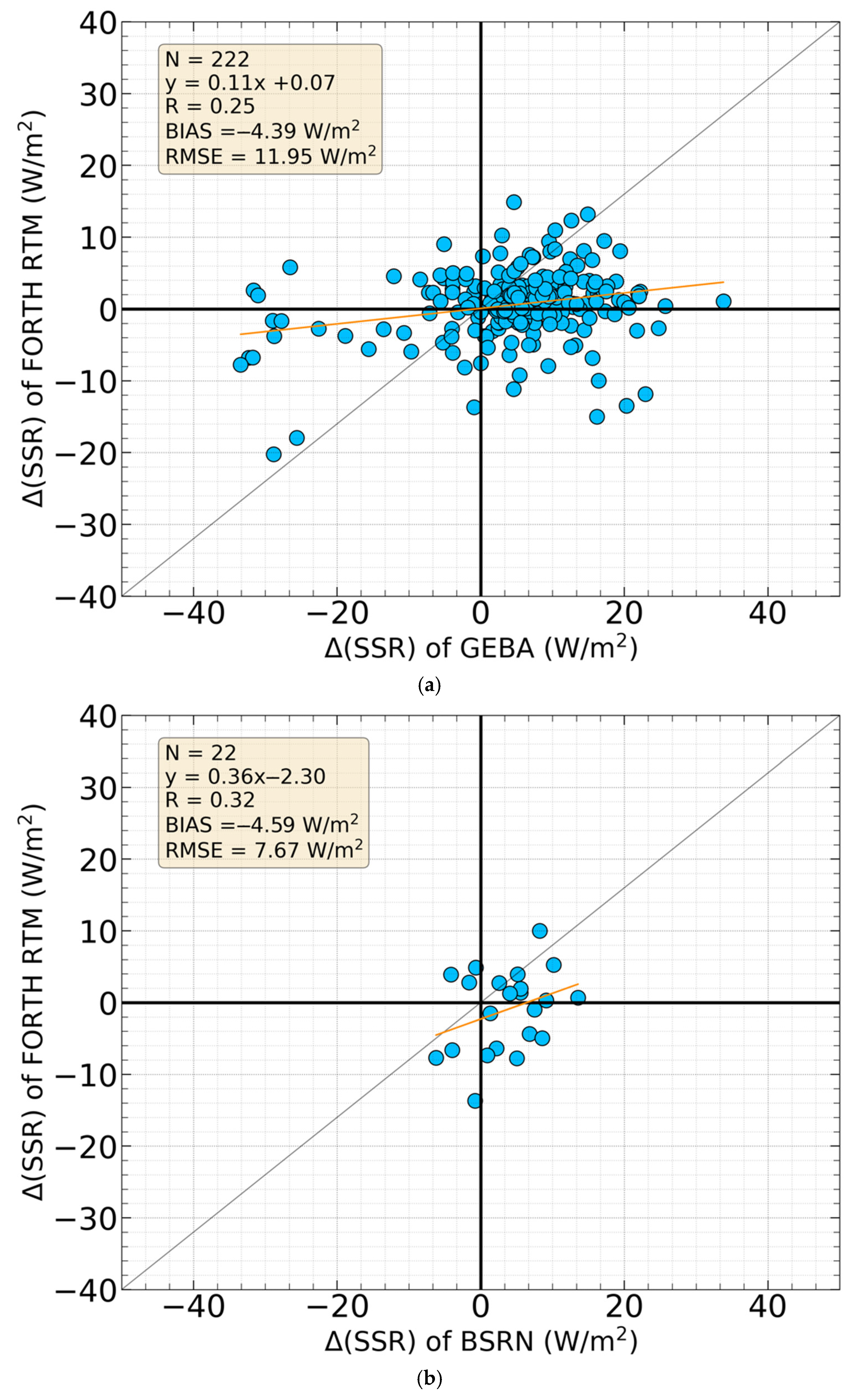
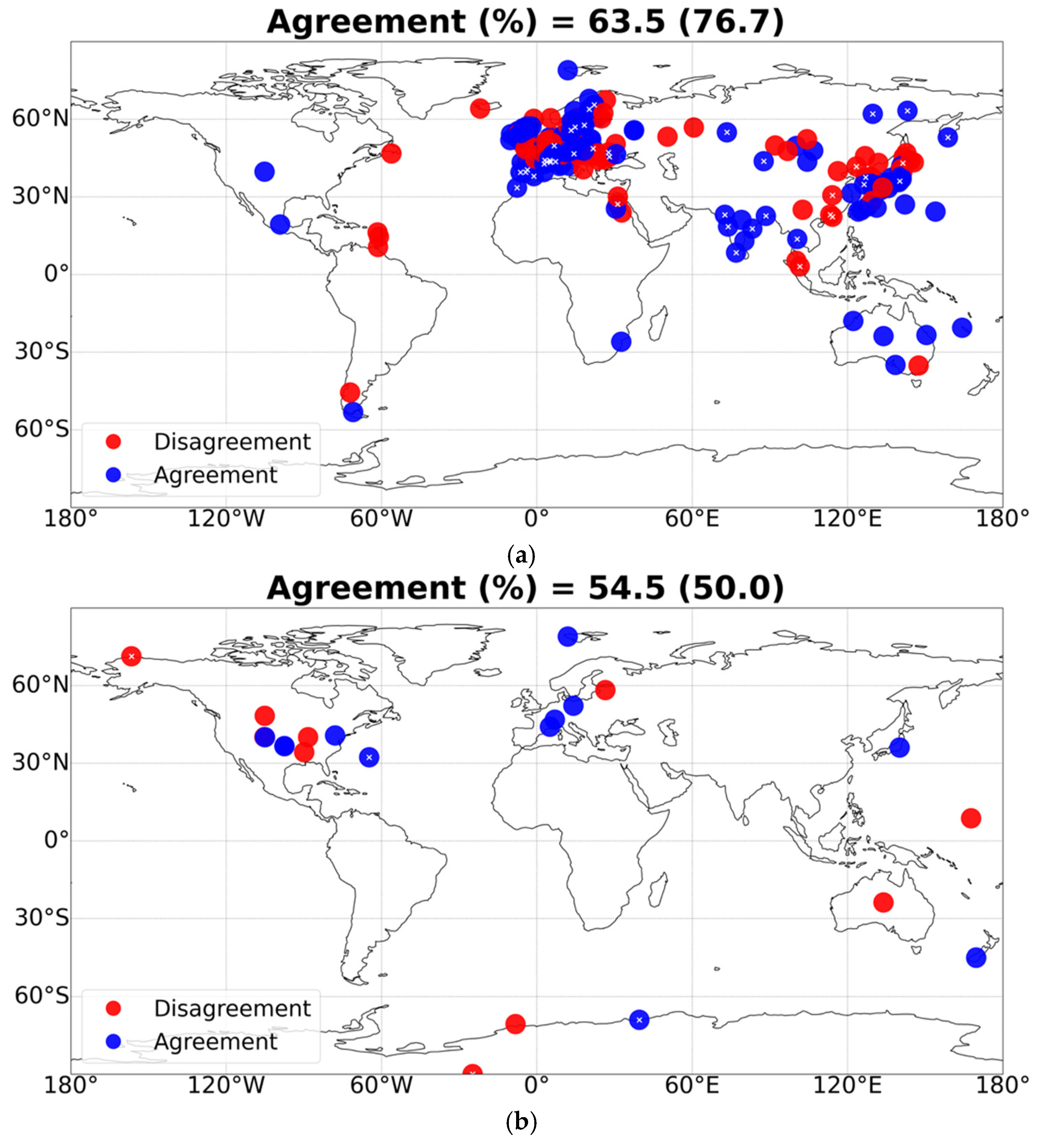
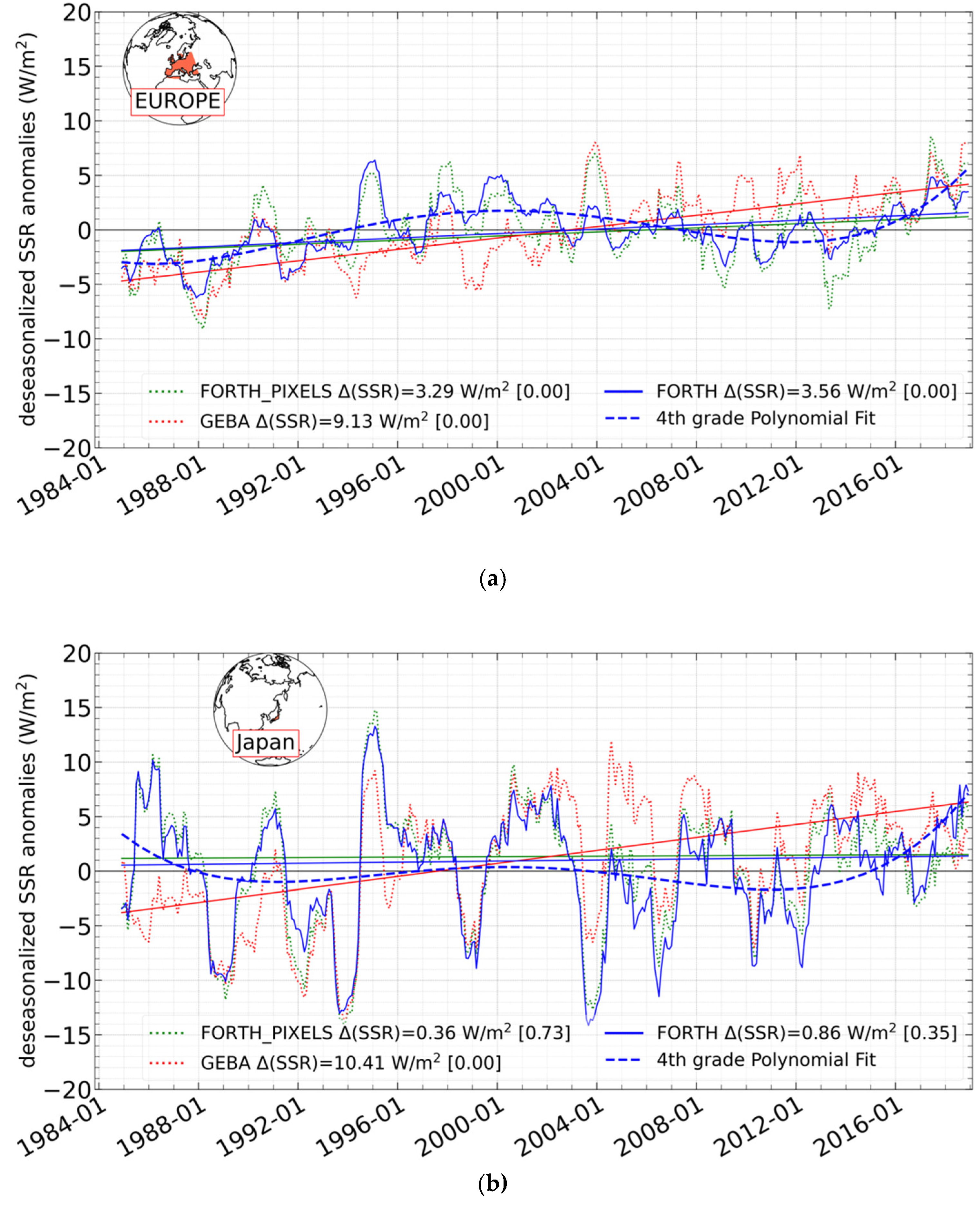
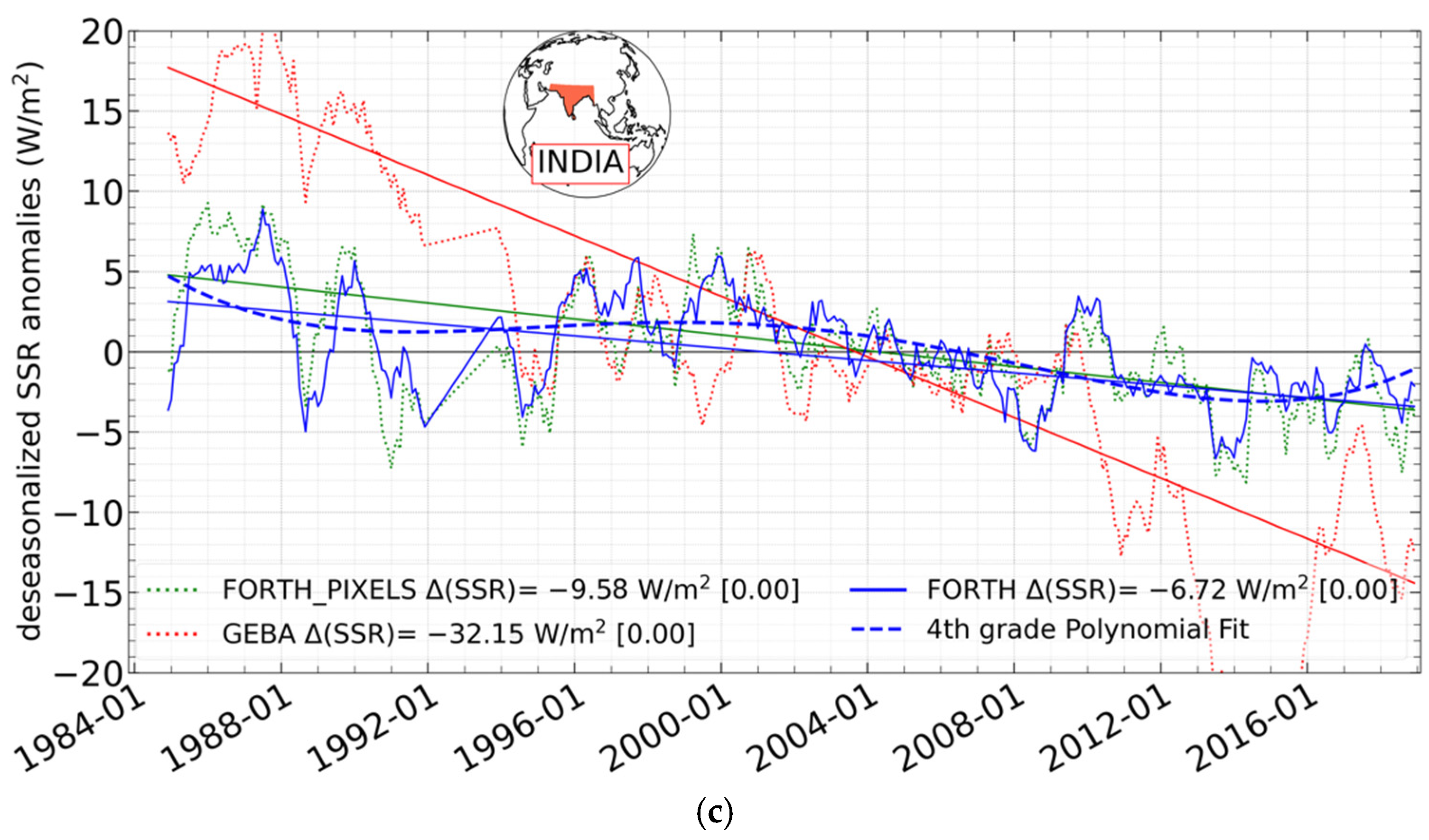
  • For the period 1984–2018, an agreement is found for 63.5% of matched model gridded and GEBA measured pairs and 54.5% of matched FORTH-RTM pixels and BSRN pairs for 1992–2018 when the sign of GDB (Δ(SSR)) for each station (222 GEBA and 22 BSRN) and the corresponding FORTH-RTM pixels is compared. For Europe, India, and Japan, there is a strong agreement between the FORTH-RTM and stations in terms of GDB signs, putting confidence in the qualitative GDB patterns in these world areas. On the other hand, the FORTH-RTM presents a weak agreement against stations in terms of the SSR changes’ magnitude. More specifically, it underestimates the brightening of most sites. This could be due to inadequate model input data, but also to issues with the stations’ measurements of their own.
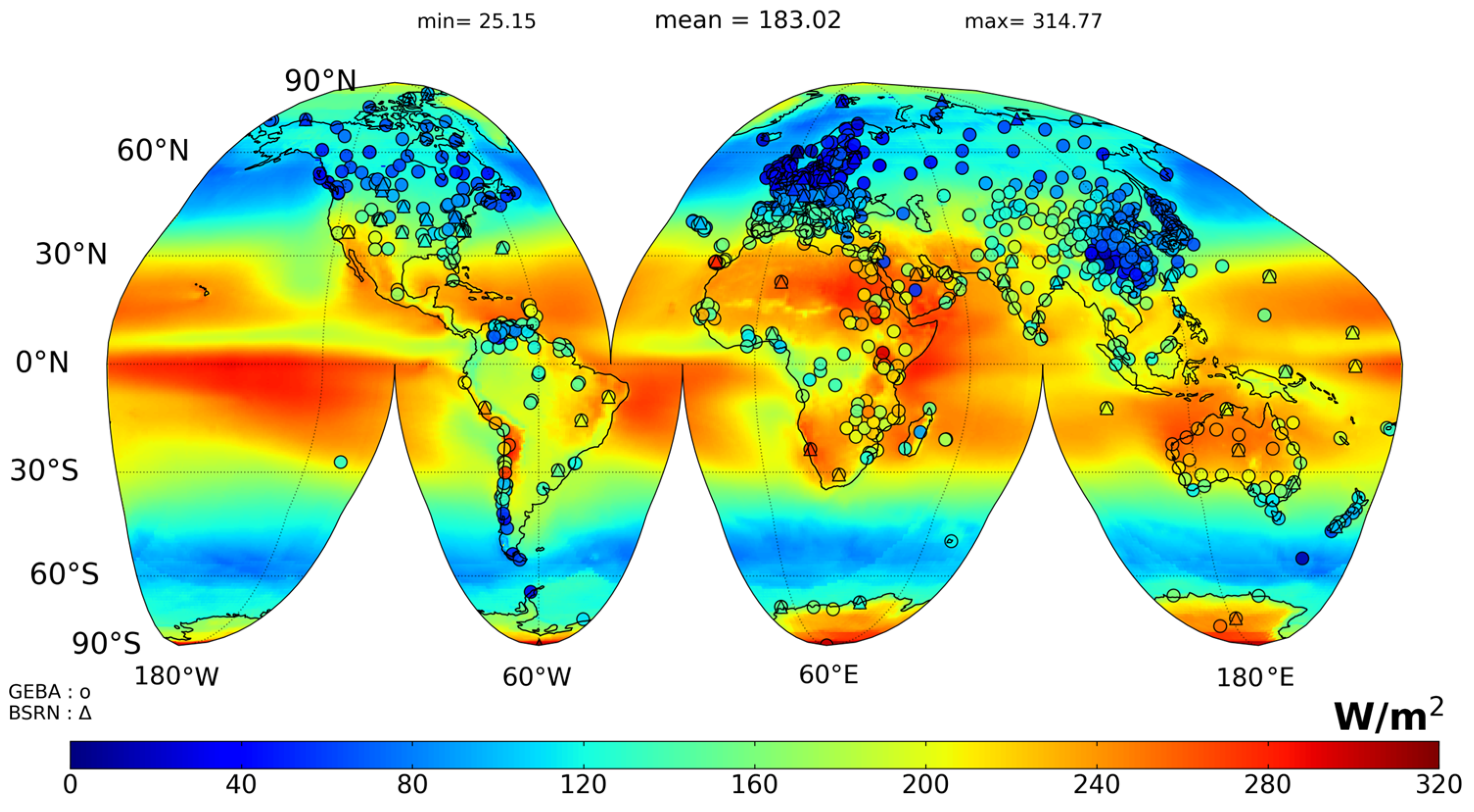
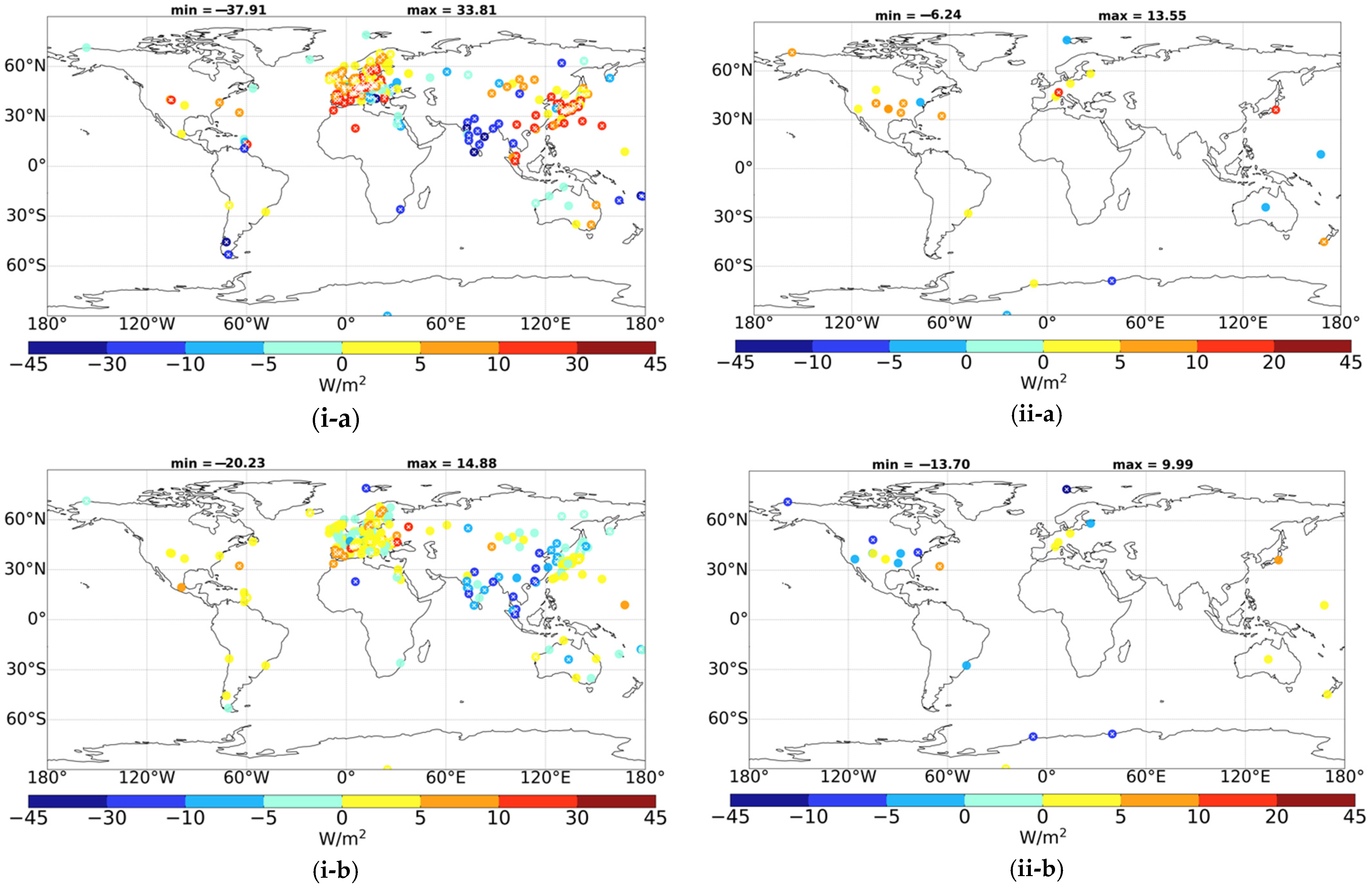
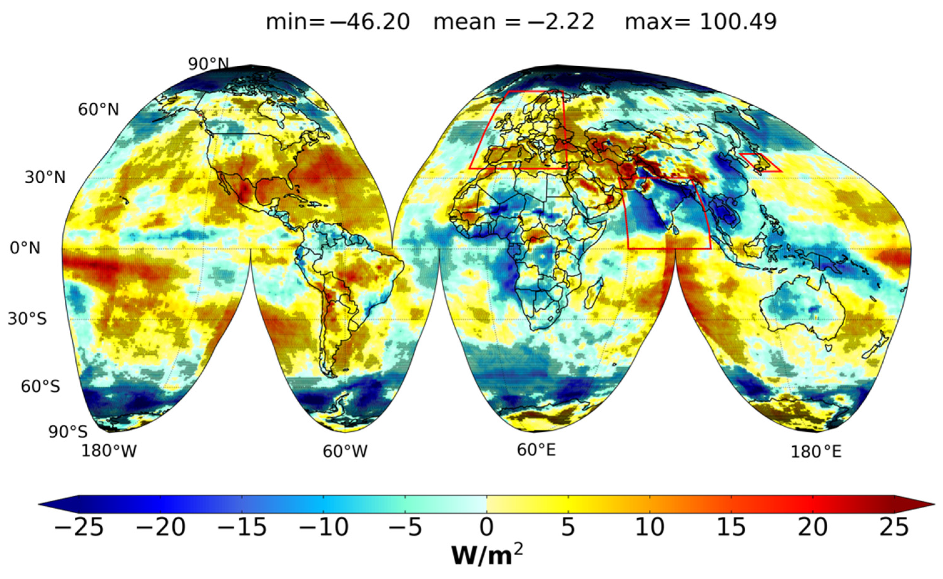
  • The computed FORTH-RTM 35-year GDB over the 01/1984–12/2018 period, reveals a statistically significant brightening in Europe, parts of Central and NW Africa, Mongolia, Mexico, parts of the tropical Pacific and sub-tropical Pacific and Atlantic Oceans, Brazil and Argentina. In contrast, statistically significant dimming is found over the western Pacific Tropical Warm Pool, India, Southeast Asia, East China, Northern South America, Australia, and some parts of oceans, especially the South Ocean. According to our calculations, different factors are responsible for GDB in different world areas. For example, AOD and cloud cover produce Europe’s brightening, while cloud optical thickness, apart from AOD induces the dimming over India and Eastern Asia. Furthermore, even for the same region, the driving factors of GDB can be different from one decade to another, thus highlighting the complexity of the phenomenon. However, it is found that globally cloud optical depth overall dominates the SSR variations.
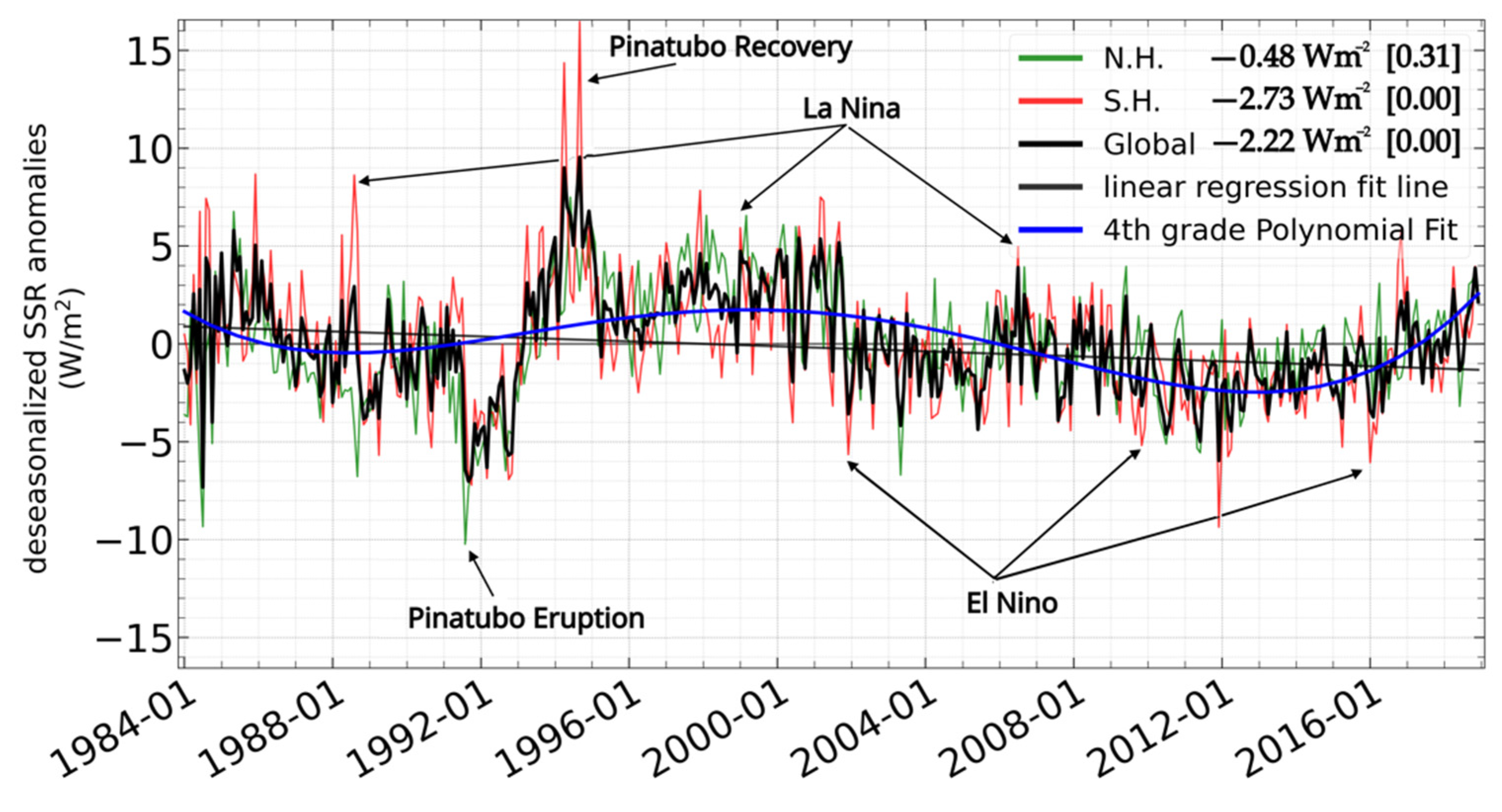
  • The FORTH-RTM SSR changes, which are affected by the ISCCP artifacts over specific limited ocean areas, show a dimming (decreasing SSR) from 1984 to 2018, equal to −2.22 Wm−2 or −0.063 Wm−2 year−1, with 53.7% of the global FORTH-RTM grids showing dimming. This dimming is found over both land and ocean areas of the globe, but oceans show a stronger dimming (−2.56 Wm−2 or −0.07 Wm−2 year−1) than land (−1.04 Wm−2 or −0.03 Wm−2 year−1). According to FORTH-RTM solar dimming also occurred on a hemispherical basis, being stronger in the Southern than Northern Hemisphere (−2.73 Wm−2 versus −0.48 Wm−2 or −0.08 Wm−2 year−1 versus −0.01 Wm−2 year−1, respectively). The SSR changes listed above are all statistically significant at the 95% confidence level (CL).
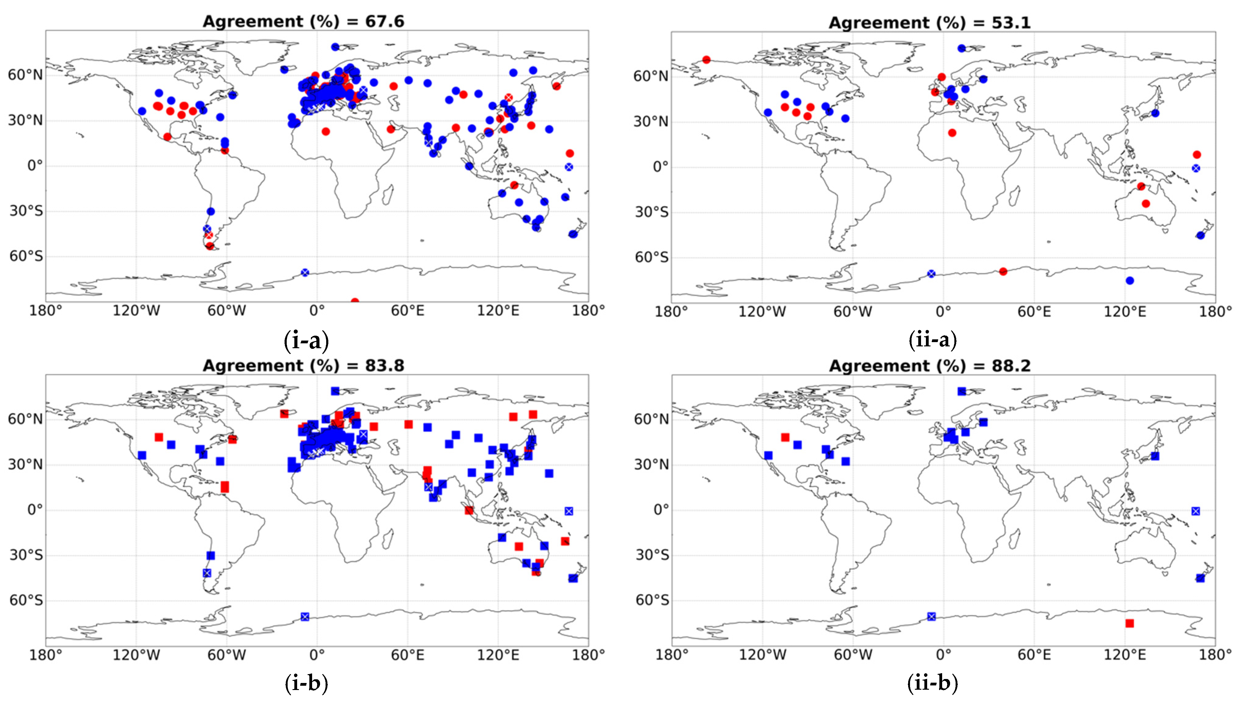
  • Examining the behavior of the agreement between the signs of GDB of GEBA stations and FORTH-RTM with time, it is found that during the 1980s, 1990s, and 2010s, the model qualitatively reproduces the GDB (dimming in the 1980s and brightening in the 1990s and 2010s) indicated by both references GEBA and BSRN station networks, exhibiting satisfactory performance. Only in the 2000s, the sign of modeled GDB is the opposite of the one suggested by stations, namely a modeled dimming against station-based brightening.
  • The brightening (5.52 Wm−2 or −0.16 Wm−2 year−1) in the 1990s estimated by the FORTH-RTM is in line with the rapid global warming driven by anthropogenic greenhouse gases. In the 2000s, when a recent hiatus has taken place, the model indicates a global dimming (−2.57 Wm−2 or −0.07 Wm−2 year−1), which seems to be in line with the deceleration of global warming. In the 2010s, FORTH-RTM suggests a global brightening (3.26 Wm−2 or 0.09 Wm−2 year−1), which is again in line with accelerated global warming. Thus, overall, the (statistically significant at the 95% CL) FORTH-RTM GDB phases seem to be consistent with the accelerating and decelerating decadal phases of global warming since 1990.
Overall, the current model (FORTH-RTM) work, based on a thorough validation against the reference global GEBA and BSRN station networks, reveals a quite satisfactory performance of the modeled absolute values of SSR, along with a less satisfactory, but still qualitatively reasonable, performance of SSR changes, i.e., GDB, during the 35-year period 1984–2018. The good performance of the model is corroborated by a satisfactory comparison of the modeled top-of-atmosphere solar fluxes against the reference CERES fluxes. The study allowed the determination of extended world areas, such as Europe, North America, India, and Japan, where the model products SSR and their changes can be considered, at least qualitatively, as accurate and reliable for further use in various applications and climatic research. On the other hand, this study highlighted areas, in particular along the tropics, where more reliable input data (cloud and aerosol) can improve the model SSR and GDB computations. In this respect, further improvements to MERRA Reanalysis aerosol optical properties and ISCCP clouds are necessary, which are nevertheless valuable given the benefits of comprehensive spatial (global), and temporal (climatological) coverage. This study highlighted the significant role of GDB in greenhouse-gas-driven global warming over four decades extending from the 1980s to 2018. Nevertheless, a longer climatology of SSR than the 35-year presented in this study is expected with the anticipated extension and improvement of the input datasets in the years to come, allowing for a better assessment of the climatic role of the GDB phenomenon, particularly in relation to the ongoing greenhouse warming.

Supplementary Materials

The following supporting information can be downloaded at: https://www.mdpi.com/article/10.3390/atmos14081258/s1, Figure S1. Global distribution of: (a) Global Energy Balance Archive (GEBA) 1545 stations and (b) Baseline Surface Radiation Network (BSRN) 73 stations, initially accessible for the evaluation of the FORTH-RTM surface solar radiation (SSR) data. The availability of each station’s monthly data in years is indicated in the color bars; Figure S2. Time periods covered by measurements of each station of (i) GEBA (1545 stations) and (ii) BSRN (73 stations) networks. Results are given for (a) the total number of stations since 1984 and (b) the number of available stations after applying criteria for computing linear slopes (see Section 2.2 of main paper), i.e., 222 GEBA and 22 BSRN stations; Figure S3. Seasonal variation of hemispherical mean correlation coefficient R between FORTH-RTM and GEBA (blue color) and between FORTH-RTM and BSRN (red color) stations, computed using SSR fluxes for the North Hemisphere (a) and the South Hemisphere (b); Figure S4. Cumulative histogram distribution of correlation coefficient R (a), bias (b), relative bias (c), root mean squared error (RMSE) (d), relative RMSE (e), between FORTH and GEBA (i, left column) and BSRN (ii, right column) stations. Results are computed using FORTH-RTM, and GEBA and BSRN station SSR fluxes, except for R, which is computed using deseasonalized SSR anomalies. the left y-axis shows the number of stations, while the right y-axis the % number of stations; Figure S5. Global distribution of correlation coefficient between FORTH-RTM and each GEBA (a, left column) and BSRN (b, right column) station SSR fluxes; Figure S6. Agreement (blue dots) and disagreement (red dots) between FORTH-RTM and station GDB (Δ(SSR)). The comparison is performed using deseasonalized anomalies for model and GEBA (left column, (i) and BSRN (right column, (ii) station fluxes per selected time periods that are characterized as Global Dimming and Brightening periods (GDB phases). The embedded white x symbols indicate statistically significant trends. At the top of each figure is indicated the percent number of stations for which there is agreement in GDB, with respect to the overall number of stations. The numbers in parentheses provide the agreement of statistically significant trends. The GDB phases (according to Wild et al., WIREsClim Change 2016, 7:91–107) are: (a) 1984–1989, (b) 1990–1999, (c) 2000–2009, (d) 2010–2018 for GEBA and (a) 1992–1999, (b) 2000–2009, (c) 2010–2018 for BSRN; Figure S7. Global distribution of FORTH-RTM GDB [Δ(SSR)] over the 35-year period 01/1984–12/2018, for (a) DJF, (b) MAM, (c) JJA, (d) SON. Reddish colors are those with positive trends (brightening), and those with bluish colors have negative trends (dimming). Statistically significant trends are indicated by black dots; Figure S8. Global distribution of the changes of model input data that are relevant to SSR and GDB, namely of: total cloud cover (a), total cloud optical thickness (b), aerosol optical depth (c), and water vapor (d) over the period 1984–2018. Bluish colors indicate decreasing trends, while yellow-reddish colors correspond to increasing trends. The statistically significant trends are denoted with black dots; Figure S9. Time series of annual global mean SSR (in blue) and model input data (in red) which are relevant with GDB: total cloud cover (a), total cloud optical thickness (b), aerosol optical depth (c) and water vapor (d) over the period 1984–2018. The associated 6th-grade polynomial fit lines are also shown.

Author Contributions

Conceptualization, N.H.; methodology, N.H. and M.S.; software, N.H., M.S., M.-B.K.-C., C.M. and I.V.; validation, N.H., M.S. and M.-B.K.-C.; formal analysis, M.S.; investigation, N.H. and M.S.; resources, N.H.; data curation, M.S.; writing—original draft preparation, M.S.; writing—review and editing, N.H., M.S., M.-B.K.-C., M.W., C.M. and I.V.; visualization, M.S. and M.-B.K.-C.; supervision, N.H.; project administration, N.H.; funding acquisition, N.H. All authors have read and agreed to the published version of the manuscript.

Funding

This research received no external funding.

Institutional Review Board Statement

Not applicable.

Informed Consent Statement

Not applicable.

Data Availability Statement

Not applicable.

Acknowledgments

We acknowledge the support of this work from the project “Dioni: Computing Infrastructure for Big-Data Processing and Analysis.” (MIS No. 5047222), which is implemented under the Action “Reinforcement of the Research and Innovation Infrastructure”, funded by the Operational Programme “Competitiveness, Entrepreneurship and Innovation” (NSRF 2014–2020) and co-financed by Greece and the European Union (European Regional Development Fund). Global dimming and brightening research at ETH Zürich got support from a sequence of Swiss National Science Foundation Grants (Grant Nos. 200021_135395, 200020_159938, 200020_188601). GEBA is co-funded by the Federal Office of Meteorology and Climatology MeteoSwiss within the framework of GCOS Switzerland. Marios-Bruno Korras-Carraca was supported by the Hellenic Foundation for Research and Innovation (H.F.R.I.) under the “2nd Call for H.F.R.I. Research Projects to support Post-Doctoral Researchers” (project acronym: ATLANTAS, project no. 544.

Conflicts of Interest

The authors declare no conflict of interest.

Abbreviations

FORTH-RTM Foundation for Research and Technology-Hellas: radiative transfer model
ISCCP International Satellite Cloud Climatology Project
MERRA-2Modern-Era Retrospective Analysis for Research and Applications v.2
GEBAGlobal Energy Balance Archive
BSRNBaseline Surface Radiation Network
SSRSurface Solar Radiation
Δ(SSR)change of SSR (equivalent to GDB)
GDBGlobal Dimming and Brightening
RPearson’s correlation coefficient
BIASmean value of FORTH-RTM minus mean value of stations
BIAS (%)100×BIAS/mean value of stations
RMSERoot Mean Squared Error
RRMSERelative Root Mean Squared Error
Mmean value of FORTH
Mimonthly (for the −i month) value of FORTH
Gmean value of stations
Gimonthly (for the −i month) value of stations
nthe number of monthly data
TOATop of the Atmosphere
OSROutgoing Solar Radiation
Δ(OSR)Changes of OSR
NHNorthern Hemisphere
SHSouthern Hemisphere

References

  1. Muneer, T.; Gueymard, C.H.K. Radiation and Daylight Models, 2nd ed.; Elsevier Butterworth Heinemann: Amsterdam, The Netherlands, 2004; pp. 13–17. [Google Scholar]
  2. Stocker, T.F.; Qin, D.; Plattner, G.-K.; Tignor, M.; Allen, S.K.; Boschung, J.; Nauels, A.; Xia, Y.; Bex, V.; Midgley, P.M. (Eds.) IPCC, 2013: Climate Change 2013: The Physical Science Basis. Contribution of Working Group I to the Fifth Assessment Report of the Intergovernmental Panel on Climate Change; Cambridge University Press: Cambridge, UK; New York, NY, USA, 2013; p. 1535. [Google Scholar]
  3. Wild, M.; Roesch, A.; Ammann, C. Global Dimming and Brightening—Evidence and Agricultural Implications. CABI Rev. 2012, 2012, 1–7. [Google Scholar] [CrossRef]
  4. Philipona, R.; Behrens, K.; Ruckstuhl, C. How Declining Aerosols and Rising Greenhouse Gases Forced Rapid Warming in Europe since the 1980s. Geophys. Res. Lett. 2009, 36, L02806. [Google Scholar] [CrossRef] [Green Version]
  5. Wang, Y.; Wild, M. A New Look at Solar Dimming and Brightening in China. Geophys. Res. Lett. 2016, 43, 11777–11785. [Google Scholar] [CrossRef]
  6. Wild, M. Decadal Changes in Radiative Fluxes at Land and Ocean Surfaces and Their Relevance for Global Warming. WIREs Clim. Chang. 2016, 7, 91–107. [Google Scholar] [CrossRef]
  7. Hatzianastassiou, N.; Ioannidis, E.; Korras-Carraca, M.-B.; Gavrouzou, M.; Papadimas, C.D.; Matsoukas, C.; Benas, N.; Fotiadi, A.; Wild, M.; Vardavas, I. Global Dimming and Brightening Features during the First Decade of the 21st Century. Atmosphere 2020, 11, 308. [Google Scholar] [CrossRef] [Green Version]
  8. Hatzianastassiou, N.; Matsoukas, C.; Fotiadi, A.; Pavlakis, K.G.; Drakakis, E.; Hatzidimitriou, D.; Vardavas, I. Global Distribution of Earth’s Surface Shortwave Radiation Budget. Atmos. Chem. Phys. 2005, 5, 2847–2867. [Google Scholar] [CrossRef] [Green Version]
  9. Liepert, B.; Romanou, A. Global Dimming and Brightening and the Water Cycle. Bull. Am. Meteorol. Soc. 2005, 86, 622–623. [Google Scholar]
  10. Wild, M.; Ohmura, A.; Makowski, K. Impact of Global Dimming and Brightening on Global Warming. Geophys. Res. Lett. 2007, 34, L04702. [Google Scholar] [CrossRef] [Green Version]
  11. Gilgen, H.; Wild, M.; Ohmura, A. Means and Trends of Shortwave Irradiance at the Surface Estimated from Global Energy Balance Archive Data. J. Clim. 1998, 11, 2042–2061. [Google Scholar] [CrossRef]
  12. Stanhill, G.; Cohen, S. Global Dimming: A Review of the Evidence for a Widespread and Significant Reduction in Global Radiation with Discussion of Its Probable Causes and Possible Agricultural Consequences. Agric. For. Meteorol. 2001, 107, 255–278. [Google Scholar] [CrossRef]
  13. Liepert, B.G. Observed Reductions of Surface Solar Radiation at Sites in the United States and Worldwide from 1961 to 1990. Geophys. Res. Lett. 2002, 29, 61-1–61-4. [Google Scholar] [CrossRef] [Green Version]
  14. Wild, M. Global Dimming and Brightening: A Review. J. Geophys. Res. Atmos. 2009, 114, D00D16. [Google Scholar] [CrossRef] [Green Version]
  15. Wild, M. Enlightening Global Dimming and Brightening. Bull. Am. Meteorol. Soc. 2012, 93, 27–37. [Google Scholar] [CrossRef]
  16. Wild, M.; Gilgen, H.; Roesch, A.; Ohmura, A.; Long, C.N.; Dutton, E.G.; Forgan, B.; Kallis, A.; Russak, V.; Tsvetkov, A. From Dimming to Brightening: Decadal Changes in Solar Radiation at Earth’s Surface. Science 2005, 308, 847–850. [Google Scholar] [CrossRef] [PubMed] [Green Version]
  17. Wild, M.; Trüssel, B.; Ohmura, A.; Long, C.N.; König-Langlo, G.; Dutton, E.G.; Tsvetkov, A. Global Dimming and Brightening: An Update beyond 2000. J. Geophys. Res. Atmos. 2009, 114, D00D13. [Google Scholar] [CrossRef] [Green Version]
  18. Norris, J.R.; Wild, M. Trends in Aerosol Radiative Effects over China and Japan Inferred from Observed Cloud Cover, Solar “Dimming,” and Solar “Brightening”. J. Geophys. Res. Atmos. 2009, 114, D00D15. [Google Scholar] [CrossRef]
  19. Ohmura, A. Observed Decadal Variations in Surface Solar Radiation and Their Causes. J. Geophys. Res. Atmos. 2009, 114, D00D05. [Google Scholar] [CrossRef] [Green Version]
  20. Badarinath, K.V.S.; Sharma, A.R.; Kaskaoutis, D.G.; Kharol, S.K.; Kambezidis, H.D. Solar Dimming over the Tropical Urban Region of Hyderabad, India: Effect of Increased Cloudiness and Increased Anthropogenic Aerosols. J. Geophys. Res. Atmos. 2010, 115, D21208. [Google Scholar] [CrossRef] [Green Version]
  21. Kambezidis, H.D. The Solar Radiation Climate of Greece. Climate 2021, 9, 183. [Google Scholar] [CrossRef]
  22. Zhang, X.; Liang, S.; Wang, G.; Yao, Y.; Jiang, B.; Cheng, J. Evaluation of the Reanalysis Surface Incident Shortwave Radiation Products from NCEP, ECMWF, GSFC, and JMA Using Satellite and Surface Observations. Remote Sens. 2016, 8, 225. [Google Scholar] [CrossRef] [Green Version]
  23. Jia, B.; Xie, Z.; Dai, A.; Shi, C.; Chen, F. Evaluation of Satellite and Reanalysis Products of Downward Surface Solar Radiation over East Asia: Spatial and Seasonal Variations. J. Geophys. Res. Atmos. 2013, 118, 3431–3446. [Google Scholar] [CrossRef]
  24. Kambezidis, H. Solar Radiation Modelling: The Latest Version and Capabilities of MRM. J. Fundam. Renew. Energy Appl. 2017, 7, E114. [Google Scholar] [CrossRef] [Green Version]
  25. Zhang, Q.; Cui, N.; Feng, Y.; Jia, Y.; Li, Z.; Gong, D. Comparative Analysis of Global Solar Radiation Models in Different Regions of China. Adv. Meteorol. 2018, 2018, 3894831. [Google Scholar] [CrossRef] [Green Version]
  26. Feng, F.; Wang, K. Determining Factors of Monthly to Decadal Variability in Surface Solar Radiation in China: Evidences from Current Reanalyses. J. Geophys. Res. Atmos. 2019, 124, 9161–9182. [Google Scholar] [CrossRef] [Green Version]
  27. Deneke, H.M.; Feijt, A.J.; Roebeling, R.A. Estimating Surface Solar Irradiance from METEOSAT SEVIRI-Derived Cloud Properties. Remote Sens. Environ. 2008, 112, 3131–3141. [Google Scholar] [CrossRef]
  28. Haywood, J.M.; Bellouin, N.; Jones, A.; Boucher, O.; Wild, M.; Shine, K.P. The Roles of Aerosol, Water Vapor and Cloud in Future Global Dimming/Brightening. J. Geophys. Res. Atmos. 2011, 116, D20203. [Google Scholar] [CrossRef] [Green Version]
  29. Ruckstuhl, C.; Norris, J.R. How Do Aerosol Histories Affect Solar “Dimming” and “Brightening” over Europe?: IPCC-AR4 Models versus Observations. J. Geophys. Res. Atmos. 2009, 114, D00D04. [Google Scholar] [CrossRef] [Green Version]
  30. Hatzianastassiou, N.; Papadimas, C.D.; Matsoukas, C.; Pavlakis, K.; Fotiadi, A.; Wild, M.; Vardavas, I. Recent Regional Surface Solar Radiation Dimming and Brightening Patterns: Inter-Hemispherical Asymmetry and a Dimming in the Southern Hemisphere. Atmos. Sci. Lett. 2012, 13, 43–48. [Google Scholar] [CrossRef]
  31. Pinker, R.T.; Zhang, B.; Dutton, E.G. Do Satellites Detect Trends in Surface Solar Radiation? Science 2005, 308, 850–854. [Google Scholar] [CrossRef] [Green Version]
  32. Hinkelman, L.M.; Stackhouse, P.W., Jr.; Wielicki, B.A.; Zhang, T.; Wilson, S.R. Surface Insolation Trends from Satellite and Ground Measurements: Comparisons and Challenges. J. Geophys. Res. Atmos. 2009, 114, D00D20. [Google Scholar] [CrossRef] [Green Version]
  33. Zhang, X.; Liang, S.; Wild, M.; Jiang, B. Analysis of Surface Incident Shortwave Radiation from Four Satellite Products. Remote Sens. Environ. 2015, 165, 186–202. [Google Scholar] [CrossRef]
  34. Wang, Z.; Zhang, M.; Wang, L.; Qin, W. A Comprehensive Research on the Global All-Sky Surface Solar Radiation and Its Driving Factors during 1980–2019. Atmos. Res. 2022, 265, 105870. [Google Scholar] [CrossRef]
  35. Romanou, A.; Liepert, B.; Schmidt, G.A.; Rossow, W.B.; Ruedy, R.A.; Zhang, Y.-C. 20th Century Changes in Surface Solar Irradiance in Simulations and Observations. Geophys. Res. Lett. 2007, 34, L05713. [Google Scholar] [CrossRef] [Green Version]
  36. Alexandri, G.; Georgoulias, A.K.; Meleti, C.; Balis, D.; Kourtidis, K.A.; Sanchez-Lorenzo, A.; Trentmann, J.; Zanis, P. A High Resolution Satellite View of Surface Solar Radiation over the Climatically Sensitive Region of Eastern Mediterranean. Atmos. Res. 2017, 188, 107–121. [Google Scholar] [CrossRef]
  37. Pfeifroth, U.; Sanchez-Lorenzo, A.; Manara, V.; Trentmann, J.; Hollmann, R. Trends and Variability of Surface Solar Radiation in Europe Based on Surface- and Satellite-Based Data Records. J. Geophys. Res. Atmos. 2018, 123, 1735–1754. [Google Scholar] [CrossRef]
  38. Sanchez-Lorenzo, A.; Enriquez-Alonso, A.; Wild, M.; Trentmann, J.; Vicente-Serrano, S.M.; Sanchez-Romero, A.; Posselt, R.; Hakuba, M.Z. Trends in Downward Surface Solar Radiation from Satellites and Ground Observations over Europe during 1983–2010. Remote Sens. Environ. 2017, 189, 108–117. [Google Scholar] [CrossRef]
  39. Dong, B.; Sutton, R.T.; Wilcox, L.J. Decadal Trends in Surface Solar Radiation and Cloud Cover over the North Atlantic Sector during the Last Four Decades: Drivers and Physical Processes. Clim. Dyn. 2023, 60, 2533–2546. [Google Scholar] [CrossRef]
  40. Wohland, J.; Brayshaw, D.; Bloomfield, H.; Wild, M. European Multidecadal Solar Variability Badly Captured in All Centennial Reanalyses except CERA20C. Environ. Res. Lett. 2020, 15, 104021. [Google Scholar] [CrossRef]
  41. Stamatis, M.; Hatzianastassiou, N.; Korras-Carraca, M.B.; Matsoukas, C.; Wild, M.; Vardavas, I. Interdecadal Changes of the MERRA-2 Incoming Surface Solar Radiation (SSR) and Evaluation against GEBA & BSRN Stations. Appl. Sci. 2022, 12, 10176. [Google Scholar] [CrossRef]
  42. Zhang, X.; Lu, N.; Jiang, H.; Yao, L. Evaluation of Reanalysis Surface Incident Solar Radiation Data in China. Sci. Rep. 2020, 10, 3494. [Google Scholar] [CrossRef] [Green Version]
  43. Hatzianastassiou, N.; Katsoulis, B.; Vardavas, I. Global Distribution of Aerosol Direct Radiative Forcing in the Ultraviolet and Visible Arising under Clear Skies. Tellus B Chem. Phys. Meteorol. 2004, 56, 51–71. [Google Scholar] [CrossRef]
  44. Hatzianastassiou, N.; Matsoukas, C.; Drakakis, E.; Stackhouse, P.W., Jr.; Koepke, P.; Fotiadi, A.; Pavlakis, K.G.; Vardavas, I. The Direct Effect of Aerosols on Solar Radiation Based on Satellite Observations, Reanalysis Datasets, and Spectral Aerosol Optical Properties from Global Aerosol Data Set (GADS). Atmos. Chem. Phys. 2007, 7, 2585–2599. [Google Scholar] [CrossRef] [Green Version]
  45. Vardavas, I.M.; Carver, J.H. Solar and Terrestrial Parameterizations for Radiative-Convective Models. Planet. Space Sci. 1984, 32, 1307–1325. [Google Scholar] [CrossRef]
  46. Joseph, J.H.; Wiscombe, W.J.; Weinman, J.A. The Delta-Eddington Approximation for Radiative Flux Transfer. J. Atmos. Sci. 1976, 33, 2452–2459. [Google Scholar] [CrossRef]
  47. Shettle, E.P.; Weinman, J.A. The Transfer of Solar Irradiance through Inhomogeneous Turbid Atmospheres Evaluated by Eddington’s Approximation. J. Atmos. Sci. 1970, 27, 1048–1055. [Google Scholar] [CrossRef]
  48. Gueymard, C.A. The Sun’s Total and Spectral Irradiance for Solar Energy Applications and Solar Radiation Models. Sol. Energy 2004, 76, 423–453. [Google Scholar] [CrossRef]
  49. Young, A.H.; Knapp, K.R.; Inamdar, A.; Hankins, W.; Rossow, W.B. The International Satellite Cloud Climatology Project H-Series Climate Data Record Product, Earth Syst. Sci. Data 2018, 10, 583–593. [Google Scholar] [CrossRef] [Green Version]
  50. Jones, P.W. First- and Second-Order Conservative Remapping Schemes for Grids in Spherical Coordinates. Monthly Weather Review. Mon. Weather Rev. 1999, 127, 2204–2210. [Google Scholar] [CrossRef]
  51. International Satellite Cloud Climatology Project (ISCCP). Climate Data Record, H-Series. Available online: https://www.ncei.noaa.gov/access/metadata/landing-page/bin/iso?id=gov.noaa.ncdc:C00956 (accessed on 2 August 2023).
  52. Randles, C.A.; Da Silva, A.M.; Buchard, V.; Colarco, P.R.; Darmenov, A.; Govindaraju, R.; Smirnov, A.; Holben, B.; Ferrare, R.; Hair, J.; et al. The MERRA-2 Aerosol Reanalysis, 1980—Onward, Part I: System Description and Data Assimilation Evaluation. J. Clim. 2017, 30, 6823–6850. [Google Scholar] [CrossRef]
  53. Korras-Carraca, M.-B.; Gkikas, A.; Matsoukas, C.; Hatzianastassiou, N. Global Clear-Sky Aerosol Speciated Direct Radiative Effects over 40 Years (1980–2019). Atmosphere 2021, 12, 1254. [Google Scholar] [CrossRef]
  54. The Second Modern-Era Retrospective Analysis for Research and Applications (MERRA-2). Available online: http://disc.sci.gsfc.nasa.gov/mdisc/ (accessed on 2 August 2023).
  55. Loeb, N.G.; Doelling, D.R.; Wang, H.; Su, W.; Nguyen, C.; Corbett, J.G.; Liang, L.; Mitrescu, C.; Rose, F.G.; Kato, S. Clouds and the Earth’s Radiant Energy System (CERES) Energy Balanced and Filled (EBAF) Top-of-Atmosphere (TOA) Edition-4.0 Data Product. J. Clim. 2018, 31, 895–918. [Google Scholar] [CrossRef]
  56. Loeb, N.G.; Priestley, K.J.; Kratz, D.P.; Geier, E.B.; Green, R.N.; Wielicki, B.A.; Hinton, P.O.; Nolan, S.K. Determination of Unfiltered Radiances from the Clouds and the Earth’s Radiant Energy System Instrument. J. Appl. Meteorol. 2001, 40, 822–835. [Google Scholar] [CrossRef]
  57. Su, W.; Corbett, J.; Eitzen, Z.; Liang, L. Next-Generation Angular Distribution Models for Top-of-Atmosphere Radiative Flux Calculation from CERES Instruments: Methodology. Atmos. Meas. Tech. 2015, 8, 611–632. [Google Scholar] [CrossRef] [Green Version]
  58. Doelling, D.R.; Loeb, N.G.; Keyes, D.F.; Nordeen, M.L.; Morstad, D.; Nguyen, C.; Wielicki, B.A.; Young, D.F.; Sun, M. Geostationary Enhanced Temporal Interpolation for CERES Flux Products. J. Atmos. Ocean. Technol. 2013, 30, 1072–1090. [Google Scholar] [CrossRef]
  59. CERES Data Products. Available online: https://Ceres.Larc.Nasa.Gov/Data/ (accessed on 30 June 2023).
  60. Michalsky, J.; Dutton, E.; Rubes, M.; Nelson, D.; Stoffel, T.; Wesely, M.; Splitt, M.; Deluisi, J.; Environmental Research; State University of New York; et al. Optimal Measurement of Surface Shortwave Irradiance Using Current Instrumentation. J. Atmos. Ocean. Technol. 1999, 16, 55–69. [Google Scholar] [CrossRef]
  61. Wild, M.; Folini, D.; Schär, C.; Loeb, N.; Dutton, E.G.; König-Langlo, G. The Global Energy Balance from a Surface Perspective. Clim. Dyn. 2013, 40, 3107–3134. [Google Scholar] [CrossRef] [Green Version]
  62. Global Energy Balance Archive. Available online: https://geba.ethz.ch/ (accessed on 2 August 2023).
  63. Driemel, A.; Augustine, J.; Behrens, K.; Colle, S.; Cox, C.; Cuevas-Agulló, E.; Denn, F.M.; Duprat, T.; Fukuda, M.; Grobe, H.; et al. Baseline Surface Radiation Network (BSRN): Structure and data description (1992–2017). Earth Syst. Sci. Data 2018, 10, 1491–1501. [Google Scholar] [CrossRef] [Green Version]
  64. World Radiation Monitoring Center (WRMC) Baseline Surface Radiation Network (BSRN). Available online: https://bsrn.awi.de/data/ (accessed on 2 August 2023).
  65. Theil, H. A Rank-Invariant Method of Linear and Polynomial Regression Analysis. In Henri Theil’s Contributions to Economics and Econometrics: Econometric Theory and Methodology; Raj, B., Koerts, J., Eds.; Springer: Dordrecht, The Netherlands, 1992; pp. 345–381. ISBN 978-94-011-2546-8. [Google Scholar]
  66. Sen, P.K. Estimates of the Regression Coefficient Based on Kendall’s Tau. J. Am. Stat. Assoc. 1968, 63, 1379–1389. [Google Scholar] [CrossRef]
  67. Mann, H.B. Nonparametric Tests Against Trend. Econometrica 1945, 13, 245–259. [Google Scholar] [CrossRef]
  68. Kendall, M.G. Rank Correlation Methods, 4th ed.; Charles Griffin: London, UK, 1975. [Google Scholar]
  69. Boudala, F.S.; Milbrandt, J.A. Evaluations of the Climatologies of Three Latest Cloud Satellite Products Based on Passive Sensors (ISCCP-H, Two CERES) against the CALIPSO-GOCCP. Remote Sens. 2021, 13, 5150. [Google Scholar] [CrossRef]
  70. Tzallas, V.; Hatzianastassiou, N.; Benas, N.; Meirink, J.F.; Matsoukas, C.; Stackhouse, P., Jr.; Vardavas, I. Evaluation of CLARA-A2 and ISCCP-H Cloud Cover Climate Data Records over Europe with ECA&D Ground-Based Measurements. Remote Sens. 2019, 11, 212. [Google Scholar]
  71. Che, H.; Gui, K.; Xia, X.; Wang, Y.; Holben, B.N.; Goloub, P.; Cuevas-Agulló, E.; Wang, H.; Zheng, Y.; Zhao, H.; et al. Large contribution of meteorological factors to inter-decadal changes in regional aerosol optical depth. Atmos. Chem. Phys. 2019, 19, 10497–10523. [Google Scholar] [CrossRef] [Green Version]
  72. Wang, Y.; Trentmann, J.; Yuan, W.; Wild, M. Validation of CM SAF CLARA-A2 and SARAH-E Surface Solar Radiation Datasets over China. Remote Sens. 2018, 10, 1977. [Google Scholar] [CrossRef] [Green Version]
  73. Baker, M.B.; Peter, T. Small-Scale Cloud Processes and Climate. Nature 2008, 451, 299–300. [Google Scholar] [CrossRef] [PubMed] [Green Version]
  74. Stensrud, D.J. Parameterization Schemes: Keys to Understanding Numerical Weather Prediction Models; Cambridge University Press: Cambridge, UK, 2007. [Google Scholar]
  75. Gavrouzou, M.; Hatzianastassiou, N.; Gkikas, A.; Korras-Carraca, M.-B.; Mihalopoulos, N. A Global Climatology of Dust Aerosols Based on Satellite Data: Spatial, Seasonal and Inter-Annual Patterns over the Period 2005–2019. Remote Sens. 2021, 13, 359. [Google Scholar] [CrossRef]
  76. Kotarba, A.Z. Evaluation of ISCCP Cloud Amount with MODIS Observations. Atmos. Res. 2015, 153, 310–317. [Google Scholar] [CrossRef]
  77. Hinkelman, L.M. The Global Radiative Energy Budget in MERRA and MERRA-2: Evaluation with Respect to CERES EBAF Data. J. Clim. 2019, 32, 1973–1994. [Google Scholar] [CrossRef]
  78. Cullather, R.I.; Bosilovich, M.G. The Energy Budget of the Polar Atmosphere in MERRA. J. Clim. 2012, 25, 5–24. [Google Scholar] [CrossRef] [Green Version]
  79. Shi, H.; Xiao, Z.; Zhan, X.; Ma, H.; Tian, X. Evaluation of MODIS and Two Reanalysis Aerosol Optical Depth Products over AERONET Sites. Atmos. Res. 2019, 220, 75–80. [Google Scholar] [CrossRef]
  80. Xia, X.A.; Wang, P.C.; Chen, H.B.; Liang, F. Analysis of Downwelling Surface Solar Radiation in China from National Centers for Environmental Prediction Reanalysis, Satellite Estimates, and Surface Observations. J. Geophys. Res. Atmos. 2006, 111, D09103. [Google Scholar] [CrossRef] [Green Version]
  81. Ma, Q.; Wang, K.; Wild, M. Impact of Geolocations of Validation Data on the Evaluation of Surface Incident Shortwave Radiation from Earth System Models. J. Geophys. Res. Atmos. 2015, 120, 6825–6844. [Google Scholar] [CrossRef] [Green Version]
  82. Campbell, G.G. View Angle Dependence of Cloudiness and the Trend in ISCCP Cloudiness. In Proceedings of the 13th Conference on Satellite Meteorology and Oceanography, Norfolk, VA, USA, 20–23 September 2004; p. 6.7. Available online: https://ams.confex.com/ams/13SATMET/techprogram/paper_79041.htm (accessed on 2 August 2023).
  83. Evan, A.T.; Heidinger, A.K.; Vimont, D.J. Arguments against a Physical Long-Term Trend in Global ISCCP Cloud Amounts. Geophys. Res. Lett. 2007, 34, L04701. [Google Scholar] [CrossRef]
  84. Norris, J.R. What Can Cloud Observations Tell Us about Climate Variability. Space Sci. Rev. 2000, 94, 375–380. [Google Scholar] [CrossRef]
  85. Norris, J.R.; Evan, A.T. Empirical Removal of Artifacts from the ISCCP and PATMOS-x Satellite Cloud Records. J. Atmos. Ocean. Technol. 2015, 32, 691–702. [Google Scholar] [CrossRef]
  86. Karlsson, K.-G.; Devasthale, A. Inter-Comparison and Evaluation of the Four Longest Satellite-Derived Cloud Climate Data Records: CLARA-A2, ESA Cloud CCI V3, ISCCP-HGM, and PATMOS-x. Remote Sens. 2018, 10, 1567. [Google Scholar] [CrossRef] [Green Version]
  87. Ramanathan, V.; Ramana, M.V.; Roberts, G.; Kim, D.; Corrigan, C.; Chung, C.; Winker, D. Warming Trends in Asia Amplified by Brown Cloud Solar Absorption. Nature 2007, 448, 575–578. [Google Scholar] [CrossRef] [PubMed]
  88. Ruckstuhl, C.; Philipona, R.; Behrens, K.; Collaud Coen, M.; Dürr, B.; Heimo, A.; Mätzler, C.; Nyeki, S.; Ohmura, A.; Vuilleumier, L.; et al. Aerosol and Cloud Effects on Solar Brightening and the Recent Rapid Warming. Geophys. Res. Lett. 2008, 35, L12708. [Google Scholar] [CrossRef] [Green Version]
  89. NOAA National Centers for Environmental Information, Climate at a Glance: Global Mapping. Available online: https://www.ncei.noaa.gov/access/monitoring/climate-at-a-glance/global/mapping (accessed on 2 August 2023).
  90. Masson-Delmotte, V.; Zhai, P.; Pirani, A.; Connors, S.L.; Péan, C.; Berger, S.; Caud, N.; Chen, Y.; Goldfarb, L.; Gomis, M.I.; et al. (Eds.) IPCC, 2021: Climate Change 2021: The Physical Science Basis. Contribution of Working Group I to the Sixth Assessment Report of the Intergovernmental Panel on Climate Change; Cambridge University Press: Cambridge, UK; New York, NY, USA,, 2021; in press. [Google Scholar] [CrossRef]
  91. Gulev, S.K.; Thorne, P.W.; Ahn, J.; Dentener, F.J.; Domingues, C.M.; Gerland, S.; Gong, D.; Kaufman, D.S.; Nnamchi, H.C.; Quaas, J.; et al. 2021: Changing State of the Climate System. In Climate Change 2021: The Physical Science Basis. Contribution of Working Group I to the Sixth Assessment Report of the Intergovernmental Panel on Climate Change; Masson-Delmotte, V., Zhai, P., Pirani, A., Connors, S.L., Péan, C., Berger, S., Caud, N., Chen, Y., Goldfarb, L., Gomis, M.I., et al., Eds.; Cambridge University Press: Cambridge, UK; New York, NY, USA,, 2021; pp. 287–422. [Google Scholar] [CrossRef]
  92. Easterling, D.R.; Wehner, M.F. Is the Climate Warming or Cooling? Geophys. Res. Lett. 2009, 36, L08706. [Google Scholar] [CrossRef] [Green Version]
  93. Foster, G.; Rahmstorf, S. Global Temperature Evolution 1979–2010. Environ. Res. Lett. 2011, 6, 044022. [Google Scholar] [CrossRef]
  94. Morice, C.P.; Kennedy, J.J.; Rayner, N.A.; Winn, J.P.; Hogan, E.; Killick, R.E.; Dunn, R.J.H.; Osborn, T.J.; Jones, P.D.; Simpson, I.R. An Updated Assessment of near-Surface Temperature Change from 1850: The HadCRUT5 Data Set. J. Geophys. Res. Atmos. 2021, 126, E2019JD032361. [Google Scholar] [CrossRef]
  95. Sanchez-Lorenzo, A.; Wild, M.; Brunetti, M.; Guijarro, J.A.; Hakuba, M.Z.; Calbó, J.; Mystakidis, S.; Bartok, B. Reassessment and Update of Long-Term Trends in Downward Surface Shortwave Radiation over Europe (1939–2012). J. Geophys. Res. Atmos. 2015, 120, 9555–9569. [Google Scholar] [CrossRef] [Green Version]
  96. Padma Kumari, B.; Goswami, B.N. Seminal Role of Clouds on Solar Dimming over the Indian Monsoon Region. Geophys. Res. Lett. 2010, 37, L06703. [Google Scholar] [CrossRef] [Green Version]
  97. Soni, V.K.; Pandithurai, G.; Pai, D.S. Is There a Transition of Solar Radiation from Dimming to Brightening over India? Atmos. Res. 2016, 169, 209–224. [Google Scholar] [CrossRef]
  98. Tanaka, K.; Ohmura, A.; Folini, D.; Wild, M.; Ohkawara, N. Is Global Dimming and Brightening in Japan Limited to Urban Areas? Atmos. Chem. Phys. 2016, 16, 13969–14001. [Google Scholar] [CrossRef] [Green Version]
Figure 1. Global Distribution of: (a) 1193 GEBA stations and (b) 66 BSRN stations, whose SSR data (availability in years indicated in the color bar) have been used in this study for the evaluation of the FORTH-RTM GDB.
Atmosphere 14 01258 g001
Figure 2. The methodology followed for the assessment/evaluation of the FORTH-RTM GDB and SSR.
Atmosphere 14 01258 g002
Figure 3. Global distribution of the long-term (1984–2018) average FORTH-RTM SSR. The average SSR of the GEBA and BSRN stations, which are used to validate the RTM, is also shown.
Atmosphere 14 01258 g003
Figure 4. Scatterplot comparison between FORTH-RTM and GEBA (i-a), and BSRN (ii-a) SSR fluxes, and between FORTH-RTM and GEBA (i-b) and BSRN (ii-b) deseasonalized SSR anomalies. The applied linear regression fit (red line), and the associated main statistical metrics, namely the equation of the applied linear fitting, the correlation coefficient (R), the root-mean-squared error (RMSE), the bias, and the total number of matched data pairs, are also shown.
Atmosphere 14 01258 g004
Figure 5. Seasonal variation of hemispherical averages of correlation coefficient R (a), bias in W/m2 (b), percent relative bias in % (c), root mean squared error (RMSE in W/m2) (d), and percent relative RMSE in % (e) between the FORTH-RTM and GEBA (blue) and BSRN (red) stations. Results, computed using SSR fluxes (except for R, which is computed using deseasonalized SSR anomalies), are given for the North Hemisphere (i-left column) and South Hemisphere (ii-right column).
Atmosphere 14 01258 g005
Figure 6. Global distribution of correlation coefficient (a), bias (b) and relative percent bias (c) root mean squared error (d), relative root mean squared error (e), computed for the comparison between FORTH-RTM and each GEBA (i, left column) and BSRN (ii, right column) station SSR fluxes, except for R that is computed using deseasonalized SSR anomalies.
Atmosphere 14 01258 g006aAtmosphere 14 01258 g006b
Figure 7. Scatterplot comparison between FORTH-RTM and GEBA (a), and FORTH-RTM and BSRN (b) Δ(SSR) or GDB (in Wm−2). The linear regression fit, and the associated statistical metrics, namely the equation of the applied linear fitting, the correlation coefficient (R), the root-mean-squared error (RMSE), the bias (FORTH-RTM minus stations), and the total number of matched data pairs, are also shown.
Atmosphere 14 01258 g007
Figure 8. Time series of 12-month moving averages of SSR anomalies for GEBA stations ((a), blue curve) and BSRN stations ((b), blue curve) along with those for the corresponding FORTH-RTM pixels (red curves). The number of available stations for each month is also shown in green color. The computed Δ(SSR) and the associated p-values for the two sets of time series (1984–2018 for GEBA and 1992–2018 for BSRN) are given at the top of each figure.
Atmosphere 14 01258 g008
Figure 9. Computed GDB (or Δ(SSR), in Wm−2) for GEBA (i-a) and BSRN (ii-a) stations and for the corresponding pixels of FORTH-RTM containing the GEBA (i-b) and BSRN (ii-b) stations. Negative values, shown in blue and green colors, indicate dimming, and positive values, in yellow, orange, and red colors, indicate brightening. The embedded white × symbols indicate trends that are statistically significant (at the 95% confidence level, assessed by applying the non-parametric Mann–Kendall test). The trends are estimated over the periods covered by each station (shown in Figure S2).
Atmosphere 14 01258 g009
Figure 10. Agreement (blue dots) and disagreement (red dots) between trends of FORTH-RTM and GEBA (a) and BSRN (b) station deseasonalized SSR anomalies. The embedded white “×” symbols indicate the statistically significant trends for both FORTH-RTM and stations. The numbers at the top of the plots provide the percentage of stations for which there is agreement/disagreement (first number) in the sign of GDB, while the corresponding numbers in parentheses refer to statistically significant trends.
Atmosphere 14 01258 g010
Figure 11. Agreement (blue dots) and disagreement (red dots) between trends of FORTH-RTM and station deseasonalized SSR anomalies (Δ(SSR)), for GEBA (i-a) and BSRN (ii-a) stations for the period 01/2001–01/2018. The stations showing agreement at the surface against GEBA stations (i-a) and BSRN stations (ii-a), also having agreement of Δ(OSR) with CERES at TOA, during the same period, are shown in (i-b,ii-b), respectively, with blue rectangles, while those having disagreement at TOA with red rectangles. The embedded white “×” symbols indicate the statistically significant trends for both FORTH-RTM and stations. At the top of each figure, the percentage number of stations (a) and CERES pixels (b) that agree in the sign of slopes with the FORTH-RTM pixels is shown.
Atmosphere 14 01258 g011
Figure 12. Global distribution of changes of FORTH-RTM GDB, namely changes of deseasonalized SSR anomalies, over the 35-year period 01/1984–12/2018. Areas shaded with reddish/bluish colors are those with positive/negative trends (brightening/dimming). Areas (pixels) with statistically significant trends are indicated by black dots. World land areas (Europe, India, and Japan) enclosed by red rectangles are characterized by homogeneous SSR trends (reference is made to them below).
Atmosphere 14 01258 g012
Figure 13. Time series of FORTH-RTM average global (black line) and hemispherical (NH and SH, green and red lines) monthly mean deseasonalized SSR anomalies for the period January 1984–December 2018. Linear regression fit line, along with associated Δ(SSR), the p-value inside the brackets, and the 4th-order polynomial fit applied to the global time series of FORTH-RTM SSR are also shown.
Atmosphere 14 01258 g013
Figure 14. Time series (01/1984–12/2018) of deseasonalized SSR anomalies for three selected world areas with homogeneous trends (see red rectangles in Figure 12), namely, Europe (a), Japan (b), and India (c). For every area, results are given based on GEBA stations (red dotted lines), the corresponding FORTH-RTM pixels (including the stations, green dotted lines), and all the FORTH-RTM pixels of the areas (blue lines). Moreover, the linearly fitted lines to each time series are also displayed with similar colors, while the blue dashed line displaying the 4th-order polynomial fit applied to the time series of FORTH-RTM SSR for the entire world areas is also shown. The SSR changes along with their p-values inside the brackets are also shown.
Atmosphere 14 01258 g014aAtmosphere 14 01258 g014b
Table 1. Comparison between FORTH-RTM and GEBA/BSRN SSR on an annual and seasonal basis (December–January–February, March–April–May, June–July–August, and September–October–November), along with the computed main statistical parameters (number of matched data pairs, N, slope value of applied linear regression fit, absolute and percent relative biases of FORTH-RTM relative to the mean GEBA/BSRN values, root mean squared error, RMSE, percent relative RMSE (RRMSE) with respect to the mean GEBA/BSRN values, correlation coefficient, R, the mean GEBA and BSRN values and the number of available stations, id, whose SSR measurements are used in the comparison). In addition, the R and slope values computed using deseasonalized SSR anomalies are given in parentheses. The percent relative bias and RMSE values are also given in parentheses.
FORTH-GEBAANNUALDJFMAMJJASON
R0.96 (0.72)0.97 (0.67)0.92 (0.74)0.90 (0.73)0.97 (0.71)
BIAS−4.71 (−2.9%)−1.52 (−1.5%)−7.26 (−3.9%)−7.26 (−3.3%)−2.63 (−2.0%)
RMSE21.02 (13.1%)18.17 (17.9%)22.86 (12.1%)24.35 (11.1%)17.77 (13.5%)
slope0.94 (0.68)0.96 (0.63)0.9 (0.68)0.89 (0.7)0.97 (0.68)
intercept4.642.111.3417.431.3
mean_FORTH156.2499.92181.07212.57128.95
mean_stations160.94101.44188.33219.83131.57
N188,41245,65847,81347,53947,402
stations11931177119011771191
FORTH-BSRNANNUALDJFMAMJJASON
R0.96 (0.80)0.96 (0.77)0.95 (0.81)0.94 (0.81)0.95 (0.82)
BIAS−14.29 (−7.7%)−16.65 (−11.1%)−17.15 (−8.6%)−12.12 (−5.2%)−11.29 (−7.0%)
RMSE27.68 (14.9%)32.76 (21.8%)26.47 (13.2%)24.28 (10.4%)26.72 (16.6%)
slope0.92 (0.82)0.87 (0.82)0.97 (0.83)0.9 (0.79)0.93 (0.84)
intercept−0.253.03−11.0311.360.42
mean_FORTH171.93133.27183.04220.71149.89
mean_stations186.22149.92200.2232.82161.19
N94622275242923422416
stations6659656365
Table 2. Agreement between the GDB (Δ(SSR)) of FORTH-RTM and GEBA stations over four different time periods. The percent number of GEBA stations for which the same sign of GDB is found with the corresponding model pixels is given, along with the average Δ(SSR) and the number of stations/pixels with brightening and dimming (shown in parentheses) for both GEBA and FORTH. Red and blue vectors indicate Brightening and Dimming, respectively.
GEBA
Periods
Agreement (%)GEBA
Δ(SSR) (W/m2)
GEBA (BRI, DIM)FORTH_Pixel Δ(SSR) (W/m2)FORTH_Pixel (BRI, DIM)
1984–198966.1 −2.51 Atmosphere 14 01258 i001(251,318)−1.03 Atmosphere 14 01258 i002(261,308)
1990–199960 1.40 Atmosphere 14 01258 i003(260,215)2.75 Atmosphere 14 01258 i004(341,134)
2000–200951.2 2.99 Atmosphere 14 01258 i005(228,104)−1.70 Atmosphere 14 01258 i006(114,218)
2010–201873.2 1.88 Atmosphere 14 01258 i007(221,118)5.18 Atmosphere 14 01258 i008(287,52)
Table 3. As in Table 2, but for BSRN stations.
BSRN
Periods
Agreement (%)BSRN
Δ(SSR) (W/m2)
BSRN
(BRI, DIM)
FORTH_Pixel
Δ(SSR) (W/m2)
FORTH_Pixel (BRI, DIM)
1992–199963.6 2.05 Atmosphere 14 01258 i009(7,4)2.14 Atmosphere 14 01258 i010(5,6)
2000–200950 0.5 Atmosphere 14 01258 i011(18,14)−0.68 Atmosphere 14 01258 i012(14,18)
2010–201865.9 0.14 Atmosphere 14 01258 i013(20,21)3.06 Atmosphere 14 01258 i014(30,11)
Table 4. Changes of FORTH-RTM deseasonalized SSR anomalies (Δ(SSR)), i.e., GDB, computed at global and hemispherical scales, as well as for land and ocean areas. Results are given for the entire 35-year period (1984–2018) as well as for four separate sub-periods. Red and blue vectors indicate solar brightening and dimming, respectively, while numbers in bold indicate trends that are statistically significant at 95% CL.
FORTH1984–20181984–19891990–19992000–20092010–2018
GLOBAL−2.22 Atmosphere 14 01258 i015−3.53 Atmosphere 14 01258 i0165.52 Atmosphere 14 01258 i017−2.57 Atmosphere 14 01258 i0183.26 Atmosphere 14 01258 i019
N.H.−0.48 Atmosphere 14 01258 i020−2.84 Atmosphere 14 01258 i0217.58 Atmosphere 14 01258 i022−2.71 Atmosphere 14 01258 i0233.43 Atmosphere 14 01258 i024
S.H.−2.73 Atmosphere 14 01258 i025−3.60 Atmosphere 14 01258 i0263.59 Atmosphere 14 01258 i027−2.46 Atmosphere 14 01258 i0282.70 Atmosphere 14 01258 i029
LAND−1.04 Atmosphere 14 01258 i030−3.56 Atmosphere 14 01258 i0315.47 Atmosphere 14 01258 i032−3.47 Atmosphere 14 01258 i0332.56 Atmosphere 14 01258 i034
LAND N.H.−0.41 Atmosphere 14 01258 i035−2.87 Atmosphere 14 01258 i0366.70 Atmosphere 14 01258 i037−3.48 Atmosphere 14 01258 i0381.51 Atmosphere 14 01258 i039
LAND S.H.−1.37 Atmosphere 14 01258 i040−2.11 Atmosphere 14 01258 i0412.76 Atmosphere 14 01258 i042−1.64 Atmosphere 14 01258 i0433.74 Atmosphere 14 01258 i044
OCEAN−2.56 Atmosphere 14 01258 i045−3.43 Atmosphere 14 01258 i0465.38 Atmosphere 14 01258 i047−2.56 Atmosphere 14 01258 i0483.41 Atmosphere 14 01258 i049
OCEAN N.H.−0.46 Atmosphere 14 01258 i050−2.11 Atmosphere 14 01258 i0518.07 Atmosphere 14 01258 i052−2.45 Atmosphere 14 01258 i0534.17 Atmosphere 14 01258 i054
OCEAN S.H.−2.83 Atmosphere 14 01258 i055−3.80 Atmosphere 14 01258 i0564.12 Atmosphere 14 01258 i057−2.60 Atmosphere 14 01258 i0582.42 Atmosphere 14 01258 i059
Disclaimer/Publisher’s Note: The statements, opinions and data contained in all publications are solely those of the individual author(s) and contributor(s) and not of MDPI and/or the editor(s). MDPI and/or the editor(s) disclaim responsibility for any injury to people or property resulting from any ideas, methods, instructions or products referred to in the content.

