Article

Simulation Study of the Lunar Spectral Irradiances and the Earth-Based Moon Observation Geometry

1
College of Geography and Environmental Sciences, Tianjin Normal University, Tianjin 300387, China
2
School of Economics and Management, Jilin Agricultural University, Changchun 130118, China
3
National Astronomical Observatory of the Chinese Academy of Sciences, Beijing 100012, China
4
College of Geoexploration Science and Technology, Jilin University, Changchun 130012, China
*
Authors to whom correspondence should be addressed.
Atmosphere 2023, 14(8), 1212; https://doi.org/10.3390/atmos14081212
Submission received: 29 June 2023 / Revised: 21 July 2023 / Accepted: 24 July 2023 / Published: 27 July 2023
(This article belongs to the Special Issue Recent Advance in Energy Budget and Earth-Atmosphere Coupling)

Abstract

:
As a radiant light source within the dynamic range of most spacecraft payloads, the Moon provides an excellent reference for on-orbit radiometric calibration. This research hinges on the precise simulation of lunar spectral irradiances and Earth-based Moon observation geometry. The paper leverages the Hapke model to simulate the temporal changes in lunar spectral irradiances, utilizing datasets obtained from the Lunar Reconnaissance Orbiter Camera (LROC). The research also details the transformation process from the lunar geographic coordinate system to the instantaneous projection coordinate system, thereby delineating the necessary observational geometry. The insights offered by this study have the potential to enhance future in-orbit spacecraft calibration procedures, thereby boosting the fidelity of data gathered from satellite observations.

1. Introduction

Satellite radiometric calibration serves as a cornerstone for the quantification of remote sensing. These calibration methods span laboratory calibration, field calibration, and cross-calibration [1,2]. Despite the prevalence of these methods, they each carry inherent limitations. Laboratory calibration, while controlled, lacks the ability to fully represent the operational environment of orbiting satellites. Field calibration, on the other hand, is influenced by variables such as atmospheric scattering and absorption, geometric discrepancies between ground measurements and satellite observations, and scale differences between ground and satellite measurement points. Significantly, for remote sensing, atmospheric influence on calibration is considerable and substantial. In contrast, the Moon, being devoid of an atmosphere and possessing a stable reflectance, presents itself as an optimal radiance source for spacecraft calibration. For the purposes of visible spectral remote sensing, the Moon’s stable reflectance and smooth spectral curve enhance its suitability. Meanwhile, for the purposes of thermal infrared remote sensing, the Moon’s high specific emissivity, akin to that of a black body, further establishes it as an excellent calibration source. Consequently, whether for short-wave or long-wave remote sensing, the Moon offers a promising light source for on-orbit radiation calibration and stability monitoring, a claim substantiated by previous research [3,4].
The use of the Moon as a reference point for satellite calibration has drawn considerable research interest [5,6,7,8,9]. At present, a range of sophisticated satellite systems and instruments from various countries play a crucial role in this field. These include the Hyperion, MODIS (Moderate Resolution Imaging Spectroradiometer) [10], Hyperion [11], GOES (Geostationary Operational Environmental Satellites) [12], SeaWiFS [13,14], S-NPP (Suomi National Polar-orbiting Partnership) [15] from the USA, Hodoyoshi-1 [16], and the FY meteorological satellite [17] from the USA, as well as Japan’s microsatellite Hodoyoshi-1 and China’s meteorological satellite series Fengyun. These satellite systems have executed observational experiments on the Moon employing a variety of payloads.
The approach of using the Moon as a reference point for satellite calibration has sparked considerable research attention [5,6,7,8,9]. At present, many satellites, inclusive of MODIS (Moderate Resolution Imaging Spectroradiometer) [10], Hyperion [11], GOES (Geostationary Operational Environmental Satellites) [12], SeaWiFS [13,14], S-NPP (Suomi National Polar-orbiting Partnership) [15] from the USA, Japan’s Hodoyoshi-1 microsatellite [16], and China’s Fengyun series of meteorological satellites [17], along with others, have carried out moon observation experiments employing diverse payloads. This international assortment of advanced satellite systems and instruments underscores the progression of global satellite technology and its role in environmental monitoring. The lunar radiance is influenced by various factors, such as lunar phase, libration, and the geometric relationships among the Sun, Earth, and the Moon. To calibrate lunar observations accurately, it is crucial to establish a lunar radiance model. Lunar radiance models can be categorized into ground-based observation models and lunar-orbiter observation models.
The ROLO model and the T2009 irradiance model are frequently employed ground-based observation models in lunar research. The T2009 model utilizes solar observed spectral irradiance data, lunar spectral reflectance data, lunar phase functions, and the spatial geometric variations among the Sun, Earth, and the Moon over time [18]. On the other hand, ROLO is a multi-spectral empirical model that performs multi-step fitting using approximately 1200 data points in 32 observation bands, but it does not provide geometric albedo information. Currently, the ROLO model is primarily used for monitoring satellite radiometric response degradation. Such models only output the total lunar radiance and are insufficient for calibrating the lunar disk’s uniformly illuminated regions. With the improvement of satellite resolution, it is becoming a trend to use disk-averaged lunar radiance calibration. For the importance of lunar photometric models, various countries have conducted research on photometric modeling using their own lunar exploration data, resulting in higher-resolution models such as the Clementine model [19], M3 model [20], SP model [21], and IIM model [22].
Both ground-based and satellite-based models have limitations, in that ground-based observations are affected by the minimum extreme phase angle during lunar eclipses, while satellite-based models do not consider multi-angle reflection characteristics. In reality, the lunar surface is non-uniform, exhibiting different reflection characteristics and surface features. Geometric albedo is calculated based on the angle of incidence, the geometric shape of the celestial body, and surface features. Differences in surface composition, particle size distribution, and topography lead to variations in the geometric albedos of observed celestial bodies, thereby impacting calibration results. These differences are especially significant in high-resolution satellite calibration processes, in which the calibration area is relatively small, and the influence of BRDF characteristics becomes more pronounced. Therefore, it is important to consider the multi-angle reflection characteristics of the Moon in lunar calibration research. Following this, it is essential to establish a precise observational geometry model for Earth–Moon space. This model plays a crucial role in providing the angle parameters required for pixel-scale Hapke models and can accurately capture the spatial geometric information of image elements.
Although research outcomes related to the observational geometry of Earth–Moon space that considered the phase angle have been published, they have predominantly focused on lunar-based observations [23,24]. Therefore, there is a need to develop a comprehensive observational geometry model specifically designed for Earth–Moon space, incorporating high-precision phase angle parameters. These empirical observations and research efforts establish a robust groundwork for using the Moon as a satellite calibration source.
In this paper, we simulate the distribution of the lunar spectral irradiances at the observation time, which is influenced by the phase of the Moon and the distances between the Sun, Earth, and the Moon. Our research question primarily grapples with two significant challenges, namely, the lunar spectral irradiances simulation and a projection transformation from the lunar geographic coordinate system to an instantaneous projection coordinate system. The Hapke bidirectional reflectance function can be utilized to simulate lunar spectral irradiances at the observation time using products from the Lunar Reconnaissance Orbiter Camera (LROC) (Tempe, AZ, USA). The projection in an instantaneous projection coordinate system can establish a mapped relationship between the transformation from the lunar geographic coordinate system and the instantaneous projection coordinate system at the observation time. It is expected that the conclusions drawn in this paper will provide support for on-orbit calibration of spacecraft in the future.

2. Materials and Methods

2.1. Data and Coordination System

2.1.1. Data Collection

In June 2009, NASA launched the Lunar Reconnaissance Orbiter (LRO), a robotic spacecraft now orbiting the Moon at an altitude of 50–200 km. The LROC, one of the instruments on board the LRO, was designed to construct the lunar global multi-spectral map [25], including wavelengths of 321, 360, 415, 566, 604, 643, and 689 nm. Global multispectral observations in seven wavelengths could be used to characterize lunar resources, in particular, ilmenite. Some products of the LROC, including the LROC Empirically Normalized Wide Angle Camera Mosaic Data Record (MDREMP) and the LROC Special Data Record Hapke Photometric Parameter Maps (SDWHAP), would be used in our research.
The SDWHAP consisted of 9 Hapke parameters (w, b, c, Bc0, hc, Bs0, hs, theta, phi) for each of the 7 bands of the Wide Angle Camera (WAC) in equirectangular projection (centered at 0° N, 0° E; 1° by 1° pixel scale) [26]. Spatially resolved near-global Hapke photometric parameter maps of the Moon have been composed from ~66,000 LROC WAC multispectral observations acquired from February 2010 to October 2011. The maps extend 0° E–360° E, and 70° N–70° S. These maps could be used to normalize the simulated reflectance at standard angles in 1° latitude by 1° longitude tiles in this research.
The MDREMP empirically normalized WAC mosaic was constructed from 137,400 color WAC images acquired from 21 January 2010 to 31 January 2013, over a broad range of lighting and viewing geometries [27]. Each pixel from the WAC observations was photometrically normalized to a standard geometry of a 30-degree incidence angle, a 0-degree emission angle, and a 30-degree phase angle, using an empirically derived global photometric function. Normalized WAC pixels for each location were combined using the median (average n = 142), so each mosaic value is using information from many observations.
In the conducted research, the Solar Spectral Irradiance (SSI) data product, specifically, the SORCE SIM Level 3 Solar Spectral Irradiance Daily Means V027 (SOR3SIMD), was utilized as the estimation tool for solar radiation energy [28]. The SOR3SIMD is constructed using measurements from the SIM instruments, which are combined into merged daily solar spectra over the spectral range from 240 to 2416 nm at a spectral resolution ranging from 1 to 27 nm. Irradiances are reported at a mean solar distance of 1 AU and zero relative line-of-sight velocity to the Sun. The SIM absolute uncertainty is approximately 2%. All of the SOR3SIMD data are arranged in a single file, in a tabular ASCII text format which can be easily imported into a spreadsheet application. The columns contain the date, Julian day, minimum wavelength, maximum wavelength, instrument mode, data version number, irradiance value, irradiance uncertainty, and data quality. The rows are arranged with data at each wavelength over the full SIM wavelength range, repeating each day for the length of the measurement period.

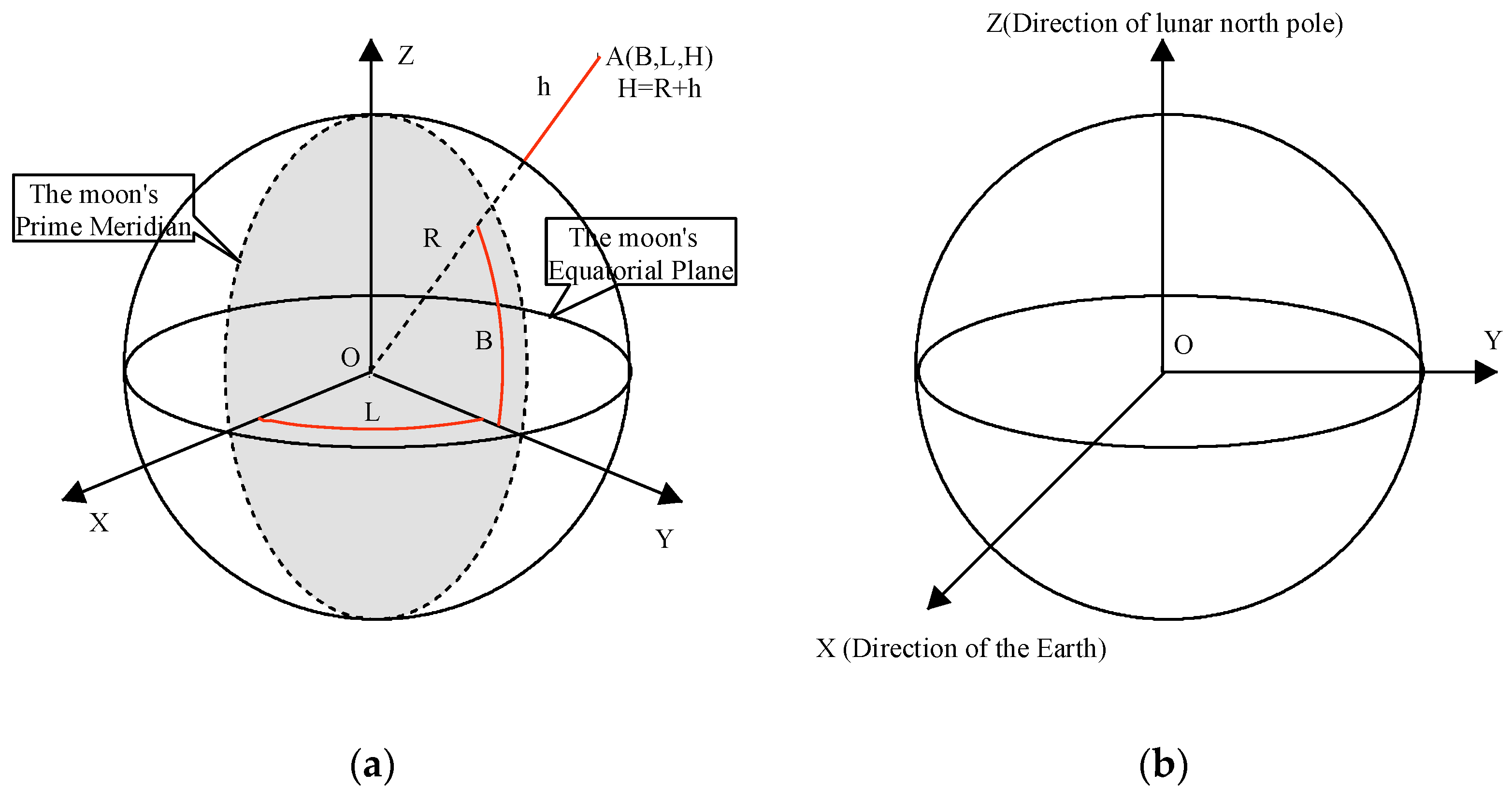
2.1.2. The Basic Coordinate System

1.
The Lunar Geographic Coordinate System
The lunar geographic coordinate system is commonly used for lunar mapping, similarly to the Earth’s geographic coordinate system. The lunar geographic coordinate system uses a three-dimensional spherical surface to define locations on the Moon. The lunar geographic coordinate system includes an angular unit of measure, a prime meridian, and a datum (based on a spheroid). The origin of the coordinates is the center of the lunar reference ellipsoid and the reference plane is the spherical reference ellipsoid sphere. The basic plane includes the lunar prime meridian and the equatorial plane. Latitude values (B) are measured relative to the equator and range from −90° at the south pole to +90° at the north pole. Longitude values (L) are measured relative to the prime meridian and range from −180° when travelling west to 180° when travelling east. The elevation (H) is defined by the distance from the reference point of the reference normal ellipsoid to the reference ellipsoid. The position of any point (A) on the Moon is referenced by its longitude, latitude, and elevation values in the lunar geographic coordinate system (Figure 1a) as ( B , L , H ) .
2.
The lunar-fixed system
The lunar-fixed system describes the location of a station on the lunar surface. The lunar-fixed system coordinate system is a right-handed Cartesian system (X, Y, Z; Figure 1b). The origin is at the lunar center of mass, the Z-axis is on the line between the north and south poles, with positive values increasing northward, and the X and Y axes are on the plane of the equator. The X-axis is found by extending from 180 degrees longitude at the equator (negative) to 0 degrees longitude (prime meridian) at the equator (positive). The Y-axis is found by extending from 90 degrees west longitude at the equator (negative) to 90 degrees east longitude at the equator (positive).
3.
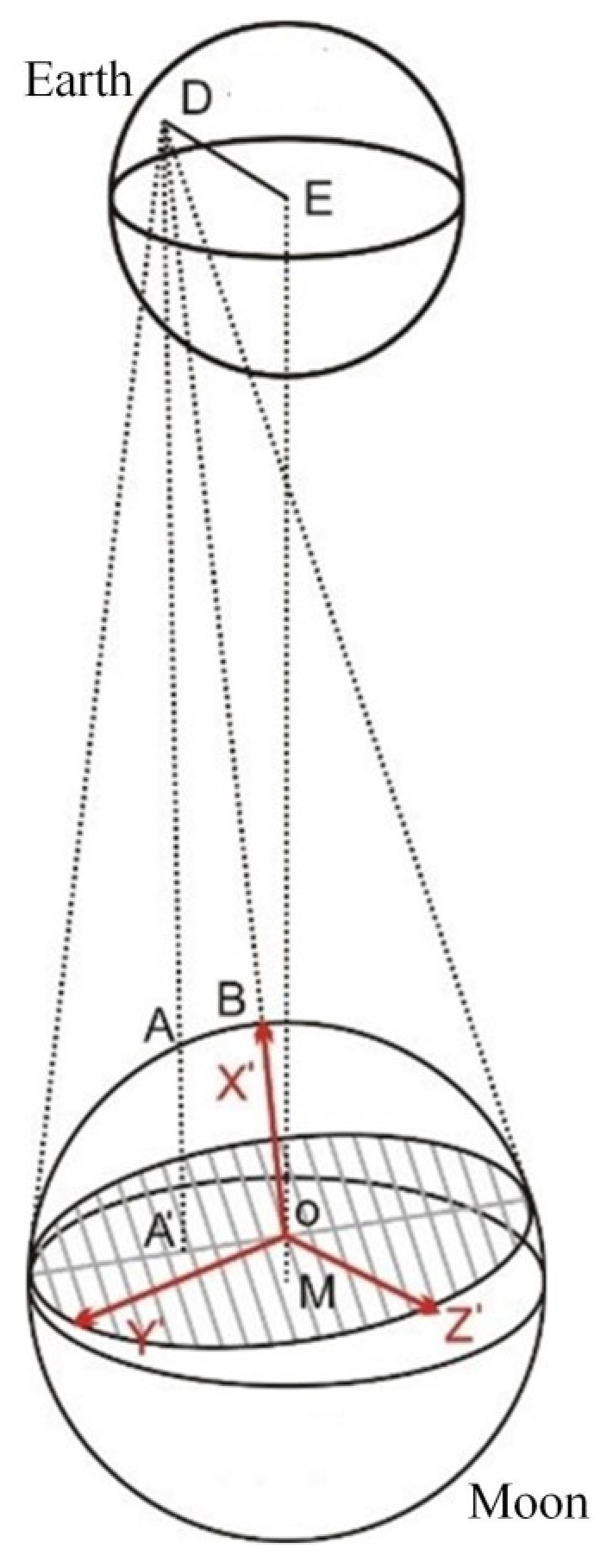
Instantaneous coordinate system
The instantaneous coordinate system is included in the instantaneous projection coordinate system (O-YZ’) and the three-dimensional instantaneous coordinate system (O-XYZ’; Figure 2). The point E is the centroid of Earth, the point M is the centroid of the Moon, the point D is an arbitrary observation point on the surface of Earth, and the shaded portion is the projection plane at the observation time (Figure 2). The origin of the instantaneous coordinate system is O, which is the intersection of the observation direction vector DM and the projection surface OYZ’. The X-axis (OX’) is in the opposite direction to the observation direction. The Y-axis (OY’) and the Z-axis (OZ’) are in the projection plane. The Y-axis is the normal vector to the plane ODE. The Z-axis could be defined using the right-hand corkscrew rule based on the direction of the X-axis and the Y-axis.

2.2. Methods

In this paper, we focus on observation simulation based on two key information sources: the lunar surface reflectance simulation and a projection transformation from the lunar geographic coordinate system to the instantaneous projection coordinate system that produced the lunar reflectance images. The Hapke model is determined for lunar surface reflectance simulation in specific frequency channels and at a specific time. The projection in an instantaneous projection coordinate system can establish a mapped relationship between transformation from the lunar geographic coordinate system and the instantaneous projection coordinate system at the observation time.

2.2.1. Hapke Model

The Hapke bidirectional reflectance model has been widely used for soil modelling. Through this model, the solution of the reflectivity in the direction of the whole Moon at the observation time can be realized. I/F, which is also called the radiance factor [29], is the ratio of the radiance observed from a surface to that of a perfectly white Lambertian surface illuminated by the same light, but at normal incidence. I is the radiance data observed from the scene, and F is the incident solar irradiance from above the Martian surface. Assuming that the shadow effect is not considered, the equation [26] is written as:
I F = L S ( i e , e e ) K w 4 [ p ( g ) ( 1 + B S 0 B S ( g ) ) + M ( i e , e e ) ] [ 1 + B C 0 B C ( g ) ]
where L S ( i e , e e ) is the Lommel–Seeliger function, i e and e e are the effective angles of incidence and emission, respectively, K is the porosity factor, w is the single scattering albedo, p(g) is the phase function, B S 0 is the amplitude of the shadow hiding opposition effect (SHOE), B S ( g ) is the SHOE function, M ( i e , e e ) is the isotropic multiple-scattering approximation (IMSA) [30,31], B C 0 is the amplitude of the coherent backscatter opposition effect (CBOE), and B C ( g ) is the coherent backscatter opposition function.
The Lommel–Seeliger function (LS) is given by:
L S ( i e , e e ) = cos ( i e ) cos ( i e ) + cos ( e e )
The phase function p(g) is given by:
p ( g ) = 1 + c 2 1 b 2 ( 1 2 b cos ( g ) + b 2 ) 3 / 2 + 1 c 2 1 b 2 ( 1 + 2 b cos ( g ) + b 2 ) 3 / 2
where b (0 ≤ b ≤ 1) is the shape-controlling parameter, and c (−1 ≤ c ≤ 1) is the relative strength of backward and forward lobes. The SHOE function B S ( g ) is given by:
B S ( g ) = 1 / [ 1 + tan ( g 2 ) / h S ]
where h S is the angular width parameter of SHOE. The IMSA function M ( i e , e e ) is given by:
M ( i e , e e ) = H ( cos ( i e ) K , w ) H ( cos ( e e ) K , w ) 1
where H ( x , w ) is Ambartsumian–Chandrasekhar H function, which is approximated by:
H ( x , w )     { 1 w x [ r 0 + 1 2 r 0 x 2 ln ( 1 + x x ) ] } 1
where r 0 is diffusive reflectance, given by:
r 0 = 1 1 w 1 + 1 w
The CBOE function B C ( g ) is given by:
B C ( g ) = 1 + 1 exp [ tan ( g 2 ) / h C ] tan ( g 2 ) / h C 2 [ 1 + tan ( g 2 ) / h C ] 2
where h C is the angular width of CBOE.

2.2.2. The Transformation Relationship of the Basic Coordinate Systems

The conversion relationship between the instantaneous projection and lunar geographic coordinate systems was obtained based on the use of the lunar fixed coordinate system as an auxiliary. The accurate conversion of lunar geographic coordinates to instantaneous projection coordinates was obtained by rotation transformation. This method involves a process of transforming lunar geodetic coordinates to lunar fixed coordinates, lunar fixed coordinates to three-dimensional instantaneous coordinates, and, finally, three-dimensional instantaneous coordinates to instantaneous projection coordinates.
1.
Transformation of lunar geodetic coordinates to lunar fixed coordinates.
The transformation from the lunar geodetic coordinate system (B, L, H) to the lunar fixed coordinate system (X, Y, Z), which both can be defined in the lunar ellipsoid, is:
{ X = ( R + h ) cos B cos L Y = ( R + h ) cos B sin L Z = ( R + h ) sin B
where X, Y, Z is the coordinate value corresponding to the lunar point in the lunar fixed system, and R is the lunar radius; L, B, and h represent the coordinate value of the lunar point in the lunar geographic coordinate system, where L is the longitude, B is the latitude, and h is the elevation.
2.
Transformation of lunar fixed coordinates to three-dimensional instantaneous coordinates.
The triaxial vector direction of the instantaneous coordinate system can be expressed in the lunar fixed coordinate system.
The component along the X-axis ( M D ):
( X X , Y Y , Z Z ) = ( X D , Y D , Z D )
The component along the Y-axis ( O Y ):
O Y = M D × M E ( X Y , Y Y , Z Y ) = ( Y D Z E Z D Y E , X E Z D X D Z E , X D Y E X E Y D )
The component along the Z-axis ( O Z ):
O Z = M B × O Y ( X Z , Y Z , Z Z ) = ( Y E Z Y Z E Y Y , X Y Z E X E Z Y , X E Y Y X Y Y E )
The origin of the instantaneous coordinate system in the lunar fixed coordinate system is derived from:
| M O | | M H | = | M H | | M D | | M O | = | M H | * | M H | | M D |
where DH is the tangent line to the Moon which passes through the observation station, OH is the radius of the lunar projection circle from the observation station at observation time, and MO is the distance of the lunar centroid and point M (Figure 3). Points O and B are both on the vector MD; the point O in the lunar fixed coordinate system is written as:
O ( O x , O y , O z ) = ( | M O | , 0 , 0 )
The instantaneous coordinate system is defined as taking the site O for origin, (Xox, Yox, Zox) for X-axis, (Xoy, Yoy, Zoy) for Y-axis, and (Xoz, Yoz, Zoz) for Z-axis. Here the triaxial unit vector of the lunar fixed coordinate system is written as:
X o x = X X X X 2 + Y X 2 + Z X 2 , Y o x = Y X X X 2 + Y X 2 + Z X 2 , Z o x = Z X X X 2 + Y X 2 + Z X 2 X o y = X Y X Y 2 + Y Y 2 + Z Y 2 , Y o y = Y Y X Y 2 + Y Y 2 + Z Y 2 , Z o y = Z Y X Y 2 + Y Y 2 + Z Y 2 X o z = X z X z 2 + Y z 2 + Z z 2 , Y o z = Y z X z 2 + Y z 2 + Z z 2 , Z o z = Z z X z 2 + Y z 2 + Z z 2
There is a simple translation relation between the instantaneous coordinate system and the lunar fixed coordinate system. M was obtained as the rotation matrix in Equation (15) from the rotation matrix:
M = [ X o x Y o x Z o x O x X o y Y o y Z o y O y X o z Y o z Z o z O z 0 0 0 1 ]
According to the definition of the rotation matrix, it can be converted to the lunar fixed coordinate system by rotation transformation in Equation (16):
( x , y , z , 1 ) = ( x , y , z , 1 ) M
where ( x , y , z ) is the target point at the lunar fixed coordinate and ( x , y , z ) is the target point at the instantaneous coordinate system.
3.
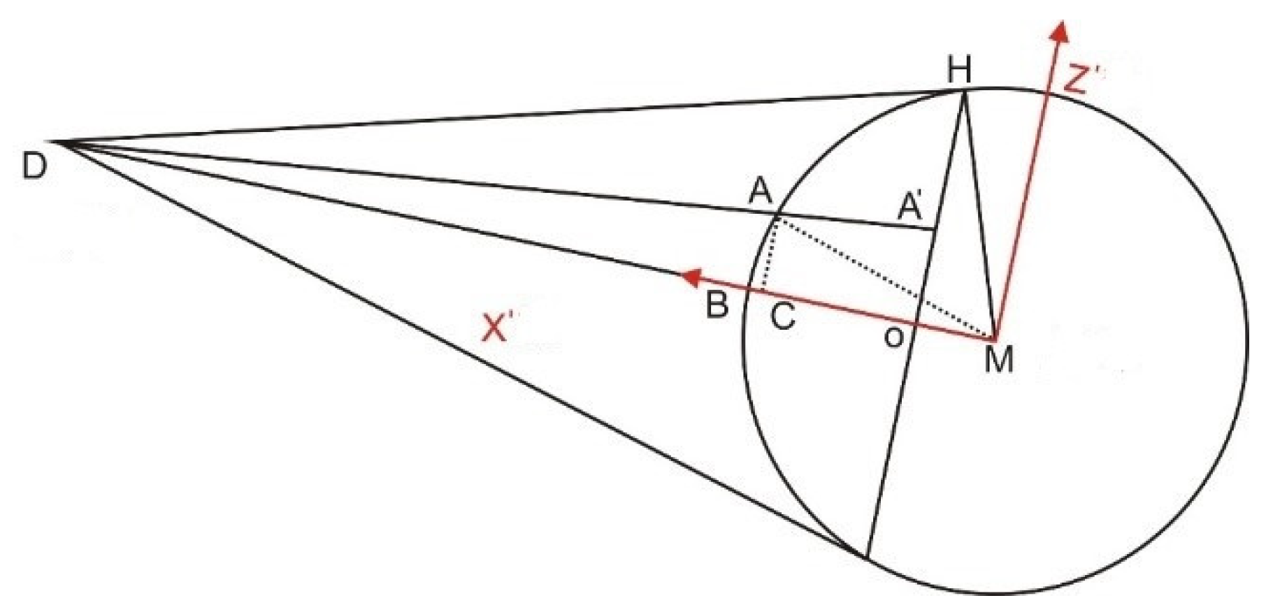
Transformation of three-dimensional instantaneous coordinates to instantaneous projection plane coordinates.
The corresponding three-dimensional instantaneous coordinates can be projected to the instantaneous projection coordinates at the observation time by a perspective projection, which is a linear projection where there are three-dimensional objects on a projection plane. In the three-dimensional instantaneous coordinate system, the linear equation of each lunar surface site at the observation time was determined to calculate the two-dimensional instantaneous projection coordinate of the target point. The linear equations of the arbitrary sampling point, A, on the lunar surface and the observation point, D, were determined to calculate the intersection coordinates of DA and the projection surface (X = 0; Figure 2). The three-dimensional instantaneous coordinate of the intersection point is ( 0 ,   Y ,   Z ) , with an instantaneous projection coordinate of ( Y ,   Z ) .

3. Results and Discussion

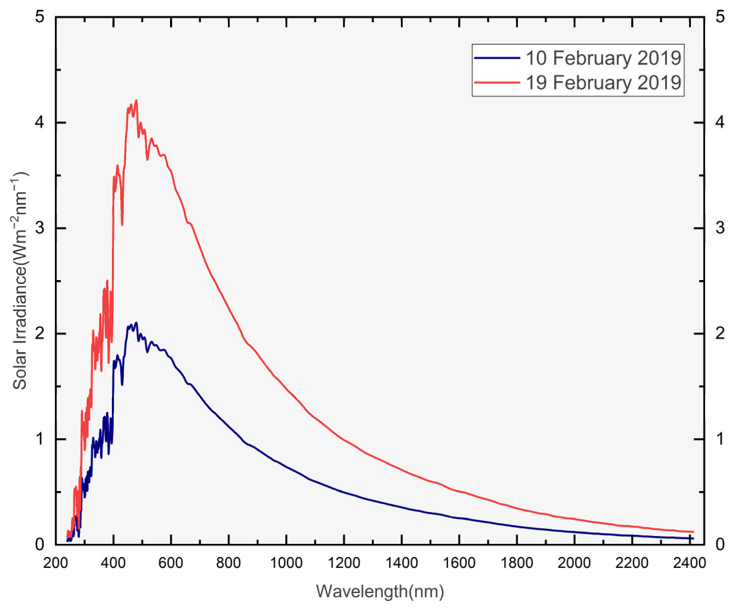
3.1. Observation Environment

The primary focus of the research’s service is on satellite calibration work involving the Moon. The influence of the atmosphere is not considered in this research. In order to facilitate the acquisition of orbital data in the study of observation geometry, ground-based observation locations are used for numerical simulation. For subsequent practical applications, when dealing with the calibration studies of non-satellite observations, it will be necessary to further incorporate atmospheric influences. The simulated observation site in the study is set in Inner Mongolia, China (115°15′1.8″ east, 42°12′42.6″ north, 1365 m altitude), which is mainly to facilitate the subsequent comparative observation requirements. However, the selection of alternative simulation observation points is also feasible, based on specific observational needs, and this selection would not impact the study’s accuracy.
The coordinates of the observation station within the lunar fixed coordinate system form the foundation for studying lunar observation geometry. Fundamental ephemerides serve as the basis for calculating planetary and lunar positions, among other related phenomena, as listed in the Astronomical Almanac. Since 2003, the Astronomical Almanac has utilized DE405/LE405 from Caltech’s Jet Propulsion Laboratory (JPL) as the fundamental planetary and lunar ephemerides. DE405/LE405 represents a set of precise computational ephemerides, curated and issued by the JPL under the auspices of the California Institute of Technology. An ephemeris, in astronomical parlance, refers to a tabulated dossier that chronicles the projected coordinates of celestial bodies and human-made satellites at specified time intervals. The DE405 model furnishes intricate details regarding the position and velocity vectors of the Sun and Moon, as well as nine primary planets (considering the classification of Pluto as a planet during the model’s conception). Supplementary data encapsulated within the DE405 ephemeris includes the Earth–Moon mass ratio, the angular radius of the Moon, and the perturbations in longitude and obliquity. In terms of temporal coverage, the DE405 data set spans an extensive epoch from 3000 BC to 3000 AD, thereby facilitating a comprehensive resource for various celestial studies and space missions.
The observation and sun coordinates for February 2019 were obtained using DE405. As representative data, observations from 10 February 2019, and 19 February 2019 were used in this study. The ground observation coordinates are (395,850,181.233, −40,592,333.726, 52,381,084.201) and (357,730,461.395, −8,793,065.875, −11,557,451.723), and the sun coordinates are (−68,763,558,072.833, 130,348,136,839.307, −1,647,761,867.411) and (146,594,202,092.887, 21,709,548,884.399, −2,268,854,787.204), respectively (Table 1).
The equation of the transformation from rectangular coordinates to spherical coordinates is written as:
α = arctan ( Y / X )         δ = arctan ( Z X 2 + Y 2 )
where α represents the latitude of the lunar subsolar point, while δ signifies the longitude of this very point. Consequently, in spherical coordinate representation, the subsolar point exhibits coordinates of (−62.2182, −0.6409) on the date of 10 February 2019, while presenting coordinates of (8.4281, −0.8776) on the subsequent date of 19 February 2019.

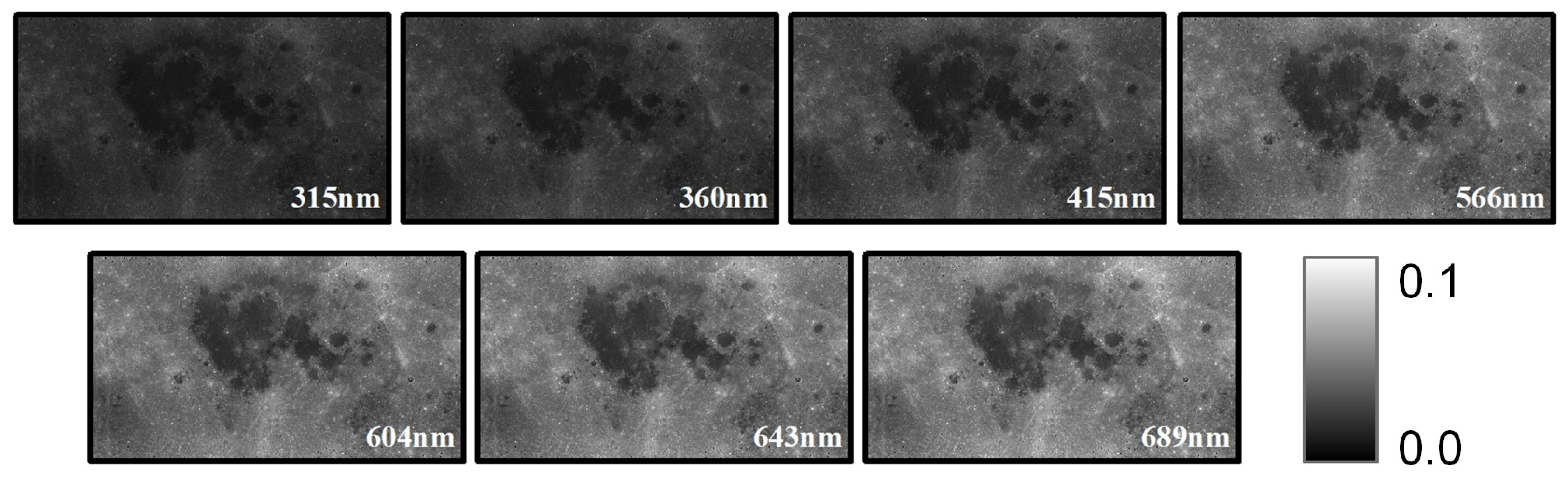
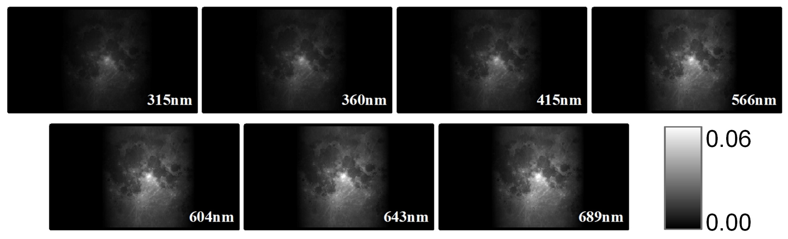
3.2. Lunar Spectral Irradiances Simulation

In order to derive the spatial distribution of the instantaneous lunar spectral radiance, it is imperative to first obtain the directional reflectance concurrent with the observation period. For this study, the empirically normalized wide angle camera mosaic data record (MDREMP), which provides the directional reflectance at an incidence angle of 30 degrees and an emission angle of 0 degrees, was utilized as the foundational dataset for reflectance simulation. Subsequently, the radiance factor, under the standard angular configuration of phase (g) = 30° and emission (e) = 0°, was computed. Moreover, the radiance factor for each pixel at the observation time was determined via the Hapke bidirectional reflectance distribution function, implemented through special data record map-projected NAC photometric products (SDRPHO) software. The standard directional reflectance and the standard radiance factor were plotted and visualized within the GCS_MOON_2000 coordinate system framework, as illustrated in Figure 4 and Figure 5, respectively.
The directional reflectance of each pixel at the observation time is affected by the observation parameters, mainly including the incident angle and the emission angle. Since the distance between Earth and the Moon is relatively large relative to the radius of the Earth, the emission angle can be approximately 0°. Consequently, the relationship of the incidence angle can be articulated through the following function:
s i n h = s i n φ s i n δ + c o s φ c o s δ c o s t
where δ is the solar declination (equal to the latitude of the subsolar point), φ is the latitude, and t is the local time, which can be obtained from the subsolar point and the longitude. The distributions of the radiance factor on 10 February 2019, and 19 February 2019 are shown in Figure A1 and Figure A2.
In particular, on 19 February 2019, the subsolar point is proximal to the prime meridian. The lunar phase approximates a full Moon, leading to elevated brightness temperature readings on the Moon’s near side. On 10 February 2019, the subsolar point’s longitude is registered at −62.2182, which coincidentally corresponds to the location of the maximum physical temperature.
The lunar spectral reflectance at the observation time can be formulated via the following expression:
R e f o b s e r v a t i o n = I / F observation I / F std R e f s t d
where I/Fstd is the radiance factor in the angle of phase (g) = incidence (i) = 30°, emission (e) = 0°, I/Fobservation is the radiance factor of each pixel at the time of observation, and Refstd is the directional reflectivity of a 30-degree incident angle and a 0-degree emission angle. The solar irradiance at the observation time is written as:
I o b s e r v a t i o n = I s t d ( 1 A U / d S u n M o o n ) 2
where d S u n M o o n signifies the Sun–Moon distance at the instant of observation and I s t d refers to the standardized solar irradiance, which is calculated at a canonical distance of 1 astronomical unit (AU) for both the Sun and Moon. The SORCE SIM Solar Spectral Irradiance data products (SOR3SIMD) reveal the solar irradiances at wavelengths of 321 nm, 360 nm, 415 nm, 566 nm, 604 nm, 643 nm, and 689 nm on 19 February 2019 to be 0.6032033, 0.9699519, 1.78526, 1.843822, 1.751854, 1.598708, and 1.453432, respectively, while those for 10 February 2019 are presented as 0.6004955, 0.9693273, 1.785617, 1.843921, 1.752042, 1.598314, and 1.453312 in Figure A3. This solar irradiance data is then used in conjunction with the lunar directional reflectance at the time of observation, yielding the distribution of the lunar surface irradiance at the corresponding observational time. This resultant distribution is portrayed in Figure 6 and Figure 7.

3.3. The Earth-Based Moon Observation Geometry

The emission angle of the lunar directional reflectance for each pixel on the lunar surface tends to vary minutely, given that the Earth–Moon distance significantly exceeds the lunar radius. To simplify the computational demand of the model, this study approximates a vertical observation scenario, that is, considers the emission angle to be 0°. In this context, the simulation primarily takes into account the impacts of the observation position and field of view.
In this context, the simulation primarily takes into account the impacts of the observation position and field of view. The transformation from lunar geographic to instantaneous projection coordinate systems allows for the determination of the projection at the observation time for 10 February 2019 (Figure 8) and 19 February 2019 (Figure 9). On 19 February 2019, simulated observation coincides with a full Moon phase, rendering a high irradiance over the majority of the lunar disc (Figure 9). On 10 February 2019, with the longitude of the subsolar point at −62.2182, more than half of the moon’s disc remains unilluminated. Consequently, the simulated lunar spectral irradiances reflect lower values, particularly on the moon’s western side (Figure 8).

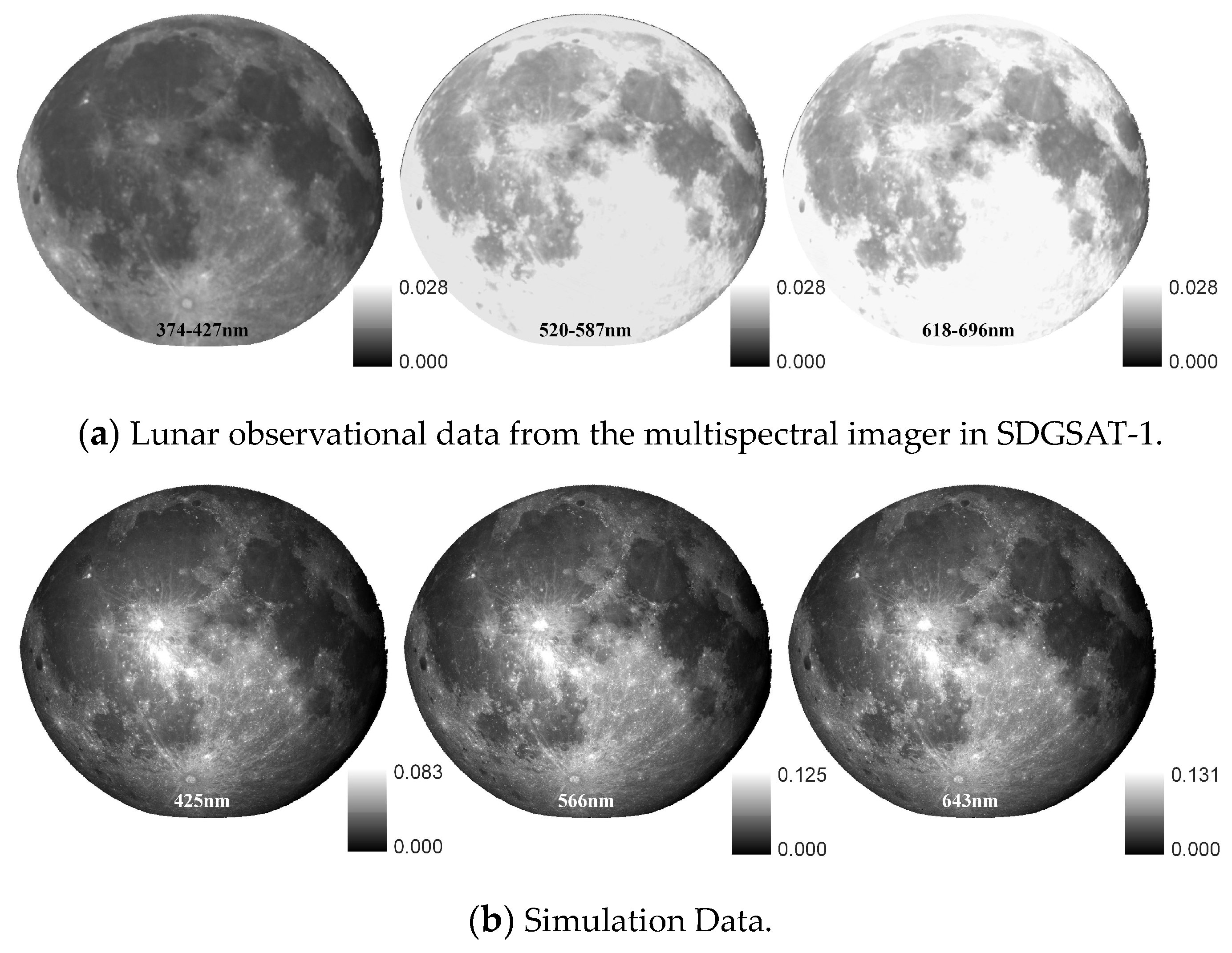
3.4. Satellite-Based Lunar Observation Verification

The Sustainable Development Goals Science Satellite 1 (SDGSAT-1), under the purview of the International Research Center of Big Data for Sustainable Development Goals (CBAS), was inaugurated in orbit on 5 November 2021. Its cardinal objective is to aggregate comprehensive data pertinent to the Sustainable Development Goals (SDGs). This data acquisition not only amplifies scientific applications but also assists the United Nations’ member states in redressing data deficits, thereby facilitating a steady and trustworthy stream of information conducive to the realization of the SDGs. SDGSAT-1, outfitted with an array of advanced sensors, including a thermal infrared spectrometer, a glimmer imager, and a multispectral imager, establishes a robust platform for meticulous observation. The intricate technical specifications of the multispectral imager in the SDGSAT-1 are encapsulated in Table 2 [32]. In this context, the 566, 643, and 415 nm bands from the Lunar Reconnaissance Orbiter Camera (LROC) can respectively map onto the deep blue, green, and red bands of the Glimmer Imager on SDGSAT-1.
This study utilized a multispectral imager for lunar observation at 3 AM on 17 February 2022. At this time, the corresponding coordinates in the lunar-fixed coordinate system for SDGAST-1 were (385,331,676.624537, −28,750,497.351839, −48,299,705.198502). The spectral reflectance from the entire simulated disk was used as a calibration standard in the study, with an assumption of consistent contribution from each pixel, thus recalibrating the distribution of reflected energy at the time of observation (Figure A4a). The simulated reflectance distribution was based on the lunar spectral irradiances simulation method and the Earth-based moon observation geometry (Figure A4b). The statistical analysis of the observed and simulated data, as shown in Figure 10, reveals a strong consistency in the overall numerical distribution. However, there were relatively more abnormal points in the simulated data, likely due to larger edge phase angles during the simulated observation process, which resulted in lower reflectance.
These reflection energy areas might not be accessible during actual observations. An error analysis was conducted, and these areas of reflected energy were eliminated to obtain an error distribution (Figure 11). The results showed that the overall error in the lunar maria areas was primarily within the range of −10% to 10%. However, in highland regions, the error was larger. This may be due to the fact that the SDWHAP data did not account for variations in surface roughness caused by terrain fluctuations. In the lunar maria areas, where the terrain is relatively flat, the bidirectional reflectance distribution function (BRDF) is stable, and the Hapke model’s simulation of lunar surface reflectance is minimally influenced by surface roughness. Concurrently, a relatively higher error, ranging from −20% to −10%, was found in the Copernicus Crater area. This might be due to the presence of different material compositions within the crater, leading to inaccuracies in the Hapke model’s parameters, and ultimately affecting the precision of the simulated reflected energy.

4. Conclusions

This research has pioneered advancements in the simulation of the distribution of instantaneous lunar spectral irradiances, and in doing so, has cultivated a comprehensive geometric model for Earth-based lunar observation. We simulated the lunar observation environment at a specific time point and a specific observation location to obtain the lunar spectral irradiances distribution within the observation field of view. This research can provide technical support for Earth-based Moon exploration and satellite radiometric calibration. The principal conclusions include:
(1)
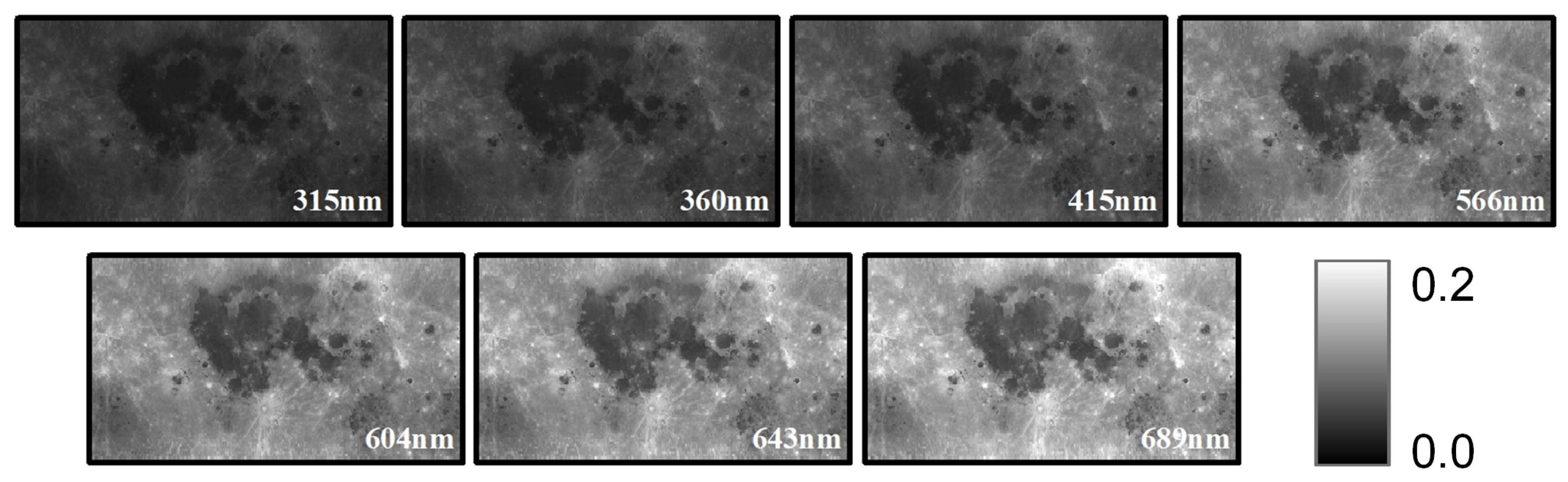
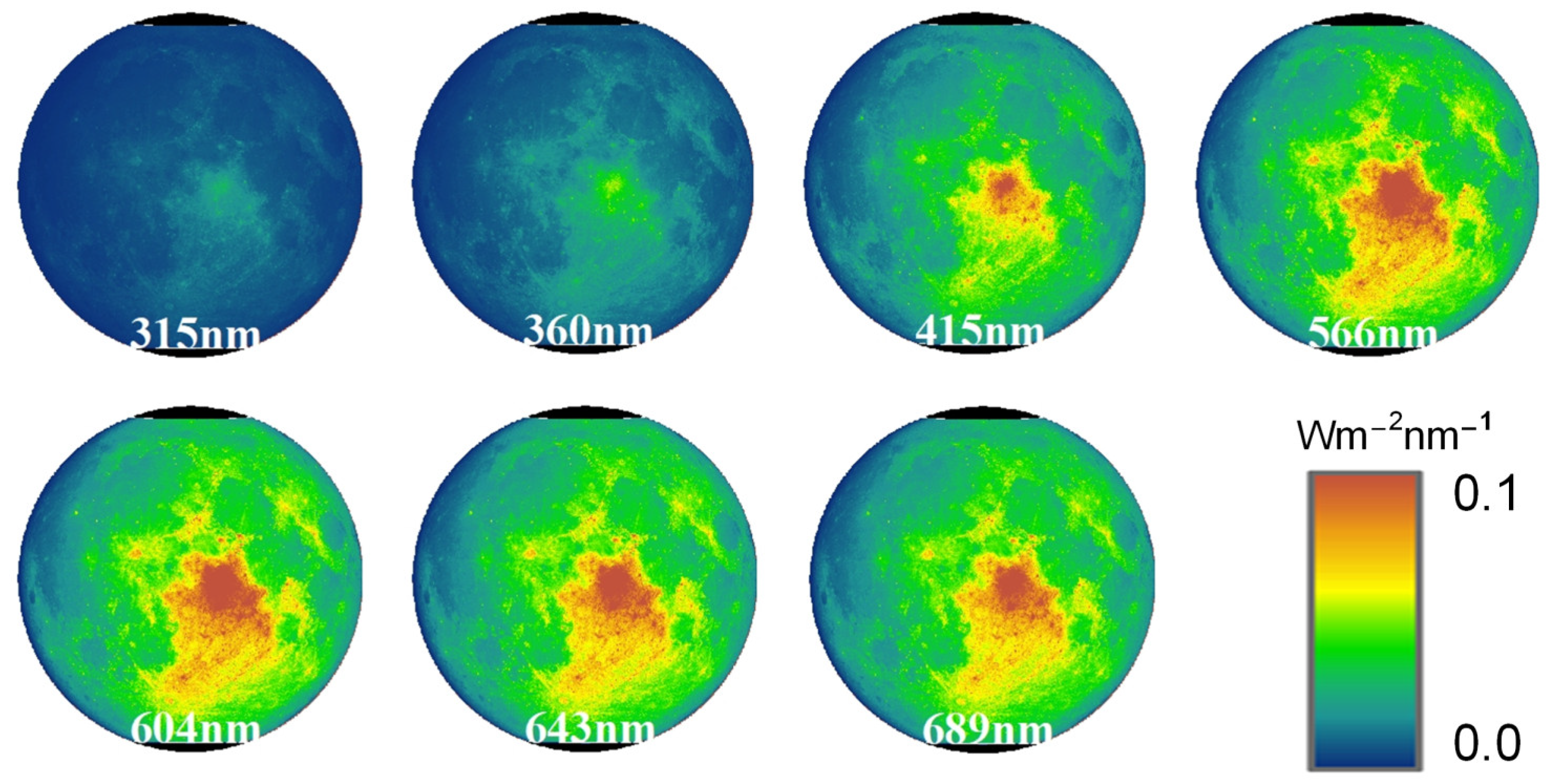
Based on the standard reflectance data and reflection factors from MDRHAP and SDRPHO products, we achieved the determination of the lunar bidirectional spectral reflectance at the observation time through the application of the Hapke bidirectional reflectance function. By aligning these findings with lunar bidirectional spectral reflectance and the SOR3SIMD product, we were able to determine the distribution of lunar spectral irradiances at the observation time, culminating in the procurement of the lunar albedo at the observation time.
(2)
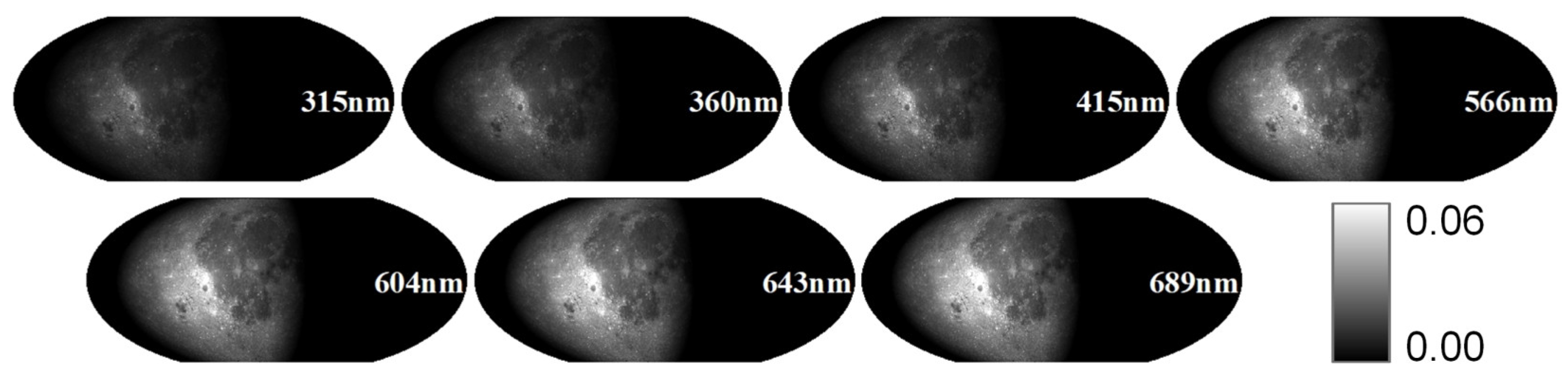
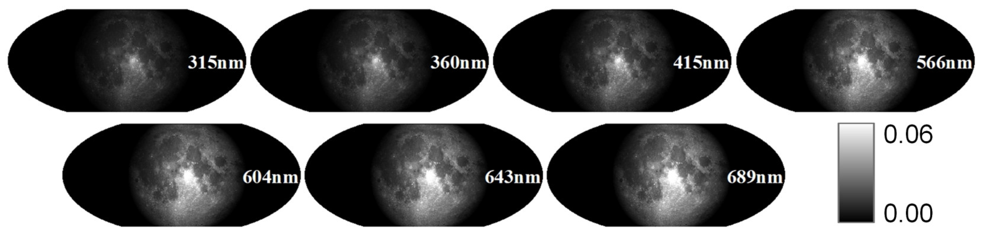
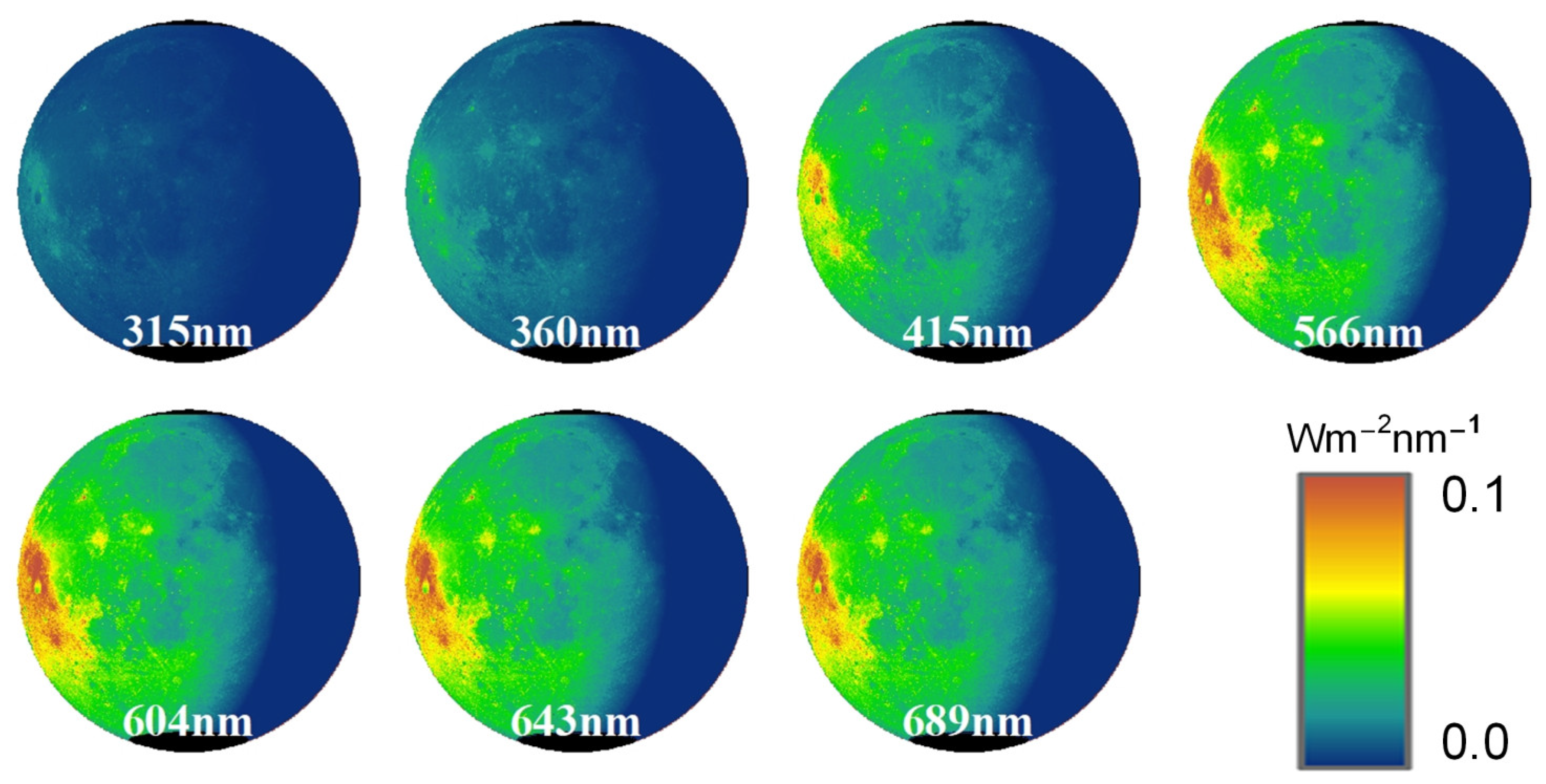
Based on the obtaining of the distribution of the lunar irradiances at the observation time, we established conversion relationships amongst different coordinate systems. These transformations included the lunar-geographic to lunar-fixed-coordinate system, lunar-fixed to instantaneous coordinate system, and instantaneous to the two-dimensional instantaneous projection plane coordinate system. Following this, the distribution of the lunar irradiances in the lunar projection plane at the observation time could be obtained quickly, conveniently, and accurately. As a summative point, this study stands as a critical benchmark in the field, constructing an intricate geometric model for Earth-based Moon observation. SDGSAT-1 was employed for lunar observation experiments, further validating the precision of the research findings.

Author Contributions

Y.L.: Software, Formal Analysis, Methodology, Writing—Original Draft, Visualization, Funding Acquisition; Q.R. and T.T.: Conceptualization, Methodology, Visualization, Supervision, Writing—Review and Editing, Funding Acquisition; H.Z., W.L. and H.G.: Data Curation, Formal Analysis; J.P. and Z.M.: Methodology, Writing—Review and Editing. All authors have read and agreed to the published version of the manuscript.

Funding

This study was funded by National Natural Science Foundation of China (Grant No. 41971306), the National Basic Survey Project (2019FY202501-03), the Foundation of Tianjin Normal University (52XB1502), and the National key research and development program of China (2021YFA0715100, 2021YFA0715101).

Institutional Review Board Statement

Not applicable.

Informed Consent Statement

Not applicable.

Data Availability Statement

The data presented in this study are available on request from the corresponding author.

Conflicts of Interest

The authors declare no conflict of interest.

Appendix A

Figure A1. The distribution of the spectral radiance factor on 10 February 2019.
Atmosphere 14 01212 g0a1
Figure A2. The distribution of the spectral radiance factor on 19 February 2019.
Atmosphere 14 01212 g0a2
Figure A3. Spectral irradiance spectral irradiance at the observation time.
Atmosphere 14 01212 g0a3
Figure A4. Lunar spectral directional reflectance on 17 February 2022.
Atmosphere 14 01212 g0a4

References

  1. Green, P.D.; Fox, N.P.; Lobb, D.; Friend, J. The traceable radiometry underpinning terrestrial and helio studies (TRUTHS) mission. In Proceedings of the SPIE 9639, Sensors, Systems, and Next-Generation Satellites XIX, Toulouse, France, 12 October 2015; Volume 96391C. [Google Scholar]
  2. Leckey, J. Climate absolute radiance and refractivity observatory (CLARREO). Int. Arch. Photogramm. Remote. Sens. Spat. Inf. Sci. 2015, XL-7/W3, 213–217. [Google Scholar]
  3. Kieffer, H.H.; Wildey, R.L. Absolute calibration of landsat instruments using the moon. Photogramm. Eng. Remote Sens. 1985, 51, 1391–1393. [Google Scholar]
  4. Kieffer, H.H. Photometric stability of the lunar surface. Icarus 1997, 130, 323–327. [Google Scholar]
  5. Kouyama, T.; Yokota, Y.; Ishihara, Y.; Nakamura, R.; Yamamoto, S.; Matsunaga, T. Development of an application scheme for the SELENE SP lunar reflectance model for radiometric calibration of hyperspectral and multispectral sensors. Planet. Space Sci. 2016, 124, 76–83. [Google Scholar]
  6. Kieffer, H.H.; Wildey, R.L. Establishing the Moon as a Spectral Radiance Standard. J. Atmos. Ocean. Technol. 1996, 13, 360–375. [Google Scholar]
  7. Kieffer, H.H.; Stone, T.C. The spectral irradiance of the moon. Astron. J. 2005, 129, 2887. [Google Scholar]
  8. Stone, T.C. Radiometric calibration stability and inter-calibration of solar-band instruments in orbit using the moon. In Proceedings of SPIE—The International Society for Optical Engineering; SPIE: Bellingham, WA, USA, 2008; Volume 7081, pp. 70810X–70810X-9. [Google Scholar]
  9. Zhang, L.; Zhang, P.; Hu, X.; Chen, L.; Min, M. A novel hyperspectral lunar irradiance model based on ROLO and mean equigonal albedo. Optik-Int. J. Light Electron Opt. 2017, 142, 657–664. [Google Scholar]
  10. Sun, J.Q.; Xiong, X.; Barnes, W.L.; Guenther, B. MODIS Reflective Solar Bands On-Orbit Lunar Calibration. IEEE Trans. Geosci. Remote Sens. 2007, 45, 2383–2393. [Google Scholar]
  11. Kieffer, H.H.; Jarecke, P.J.; Pearlman, J. Initial lunar calibration observations by the EO-1 Hyperion imaging spectrometer. In Proceedings of SPIE—The International Society for Optical Engineering; SPIE: Bellingham, WA, USA, 2002; Volume 4480, pp. 243–253. [Google Scholar]
  12. Stone, T.C.; Kieffer, H.H.; Grant, I.F. Potential for calibration of geostationary meteorological satellite imagers using the Moon. In Proceedings of SPIE—The International Society for Optical Engineering; SPIE: Bellingham, WA, USA, 2005; Volume 5882, pp. 58820P-1–58820P-9. [Google Scholar]
  13. Barnes, R.A.; Eplee, R.E.; Patt, F.S., Jr.; McClain, C.R. Changes in the radiometric sensitivity of SeaWiFS determined from lunar and solar-based measurements. Appl. Opt. 1999, 38, 4649–4664. [Google Scholar]
  14. Barnes, W.; Xiong, X.; Eplee, R.; Sun, J.; Lyu, C.-H. Use of the Moon for Calibration and Characterization of MODIS, SeaWiFS, and VIRS. Neuropharmacology 2006, 30, 1269–1274. [Google Scholar]
  15. Xiong, X.; Butler, J.; Chiang, K.; Efremova, B.; Fulbright, J.; Lei, N.; McIntire, J.; Oudrari, H.; Wang, Z.; Wu, A. Assessment of S-NPP VIIRS On-Orbit Radiometric Calibration and Performance. Remote Sens. 2016, 8, 84. [Google Scholar] [PubMed] [Green Version]
  16. Kouyama, T.; Kato, S.; Miyashita, N. One-year lunar calibration result of Hodoyoshi-1, Moon as an ideal target for small satellite radiometric calibration. In Proceedings of the 32nd Annual AIAA/USU Conference on Small Satellites, Logan, UT, USA, 4–9 August 2018. [Google Scholar]
  17. Wu, R.H.; Zhang, P.; Yang, Z.D.; Hu, X.Q.; Ding, L.; Chen, L. Monitor the radiance calibration of the remotesensing instrument by using the reflected lunar irradiance. J. Remote Sens. 2016, 20, 278–289. [Google Scholar]
  18. Miller, S.D.; Turner, R.E. A dynamic lunar spectral irradiance data set for NPOESS/VIIRS day/night band nighttime environmental applications. IEEE Trans. Geosci. Remote Sens. 2009, 47, 2316–2329. [Google Scholar]
  19. Hillier, J.K.; Buratti, B.J.; Hill, K. Multispectral photometry of the Moon and absolute calibration of the Clementine UV/Vis camera. Icarus 1999, 141, 205–225. [Google Scholar]
  20. Besse, S.; Sunshine, J.; Staid, M.; Boardman, J.; Pieters, C.; Guasqui, P.; Malaret, E.; McLaughlin, S.; Yokota, Y.; Li, J.-Y. A visible and near-infrared photometric correction for Moon Mineralogy Mapper (M3). Icarus 2013, 222, 229–242. [Google Scholar]
  21. Yokota, Y.; Matsunaga, T.; Ohtake, M.; Haruyama, J.; Nakamura, R.; Yamamoto, S.; Ogawa, Y.; Morota, T.; Honda, C.; Saiki, K.; et al. Lunar photometric properties at wavelengths 0.5–1.6 μm acquired by SELENE Spectral Profiler and their dependency on local albedo and latitudinal zones. Icarus 2011, 215, 639–660. [Google Scholar]
  22. Wu, Y.; Besse, S.; Li, J.Y.; Combe, J.P.; Wang, Z.; Zhou, X.; Wang, C. Photometric correction and in-flight calibration of Chang’E-1 Interference Imaging Spectrometer (IIM) data. Icarus 2013, 222, 283–295. [Google Scholar]
  23. Guo, H.; Ye, H.; Liu, G.; Dou, C.; Huang, J. Error analysis of exterior orientation elements on geolocation for a Moon-based Earth observation optical sensor. Int. J. Digit. Earth 2018, 13, 374–392. [Google Scholar]
  24. Li, T.; Guo, H.; Zhang, L.; Nie, C.; Liao, J.; Liu, G. Simulation of Moon-based Earth observation optical image processing methods for global change study. Front. Earth Sci. 2020, 14, 236–250. [Google Scholar]
  25. Robinson, M.S.; Brylow, S.M.; Tschimmel, M.; Humm, D.; Lawrence, S.J.; Thomas, P.C.; Denevi, B.W.; Bowman-Cisneros, E.; Zerr, J.; Ravine, M.A.; et al. Lunar reconnaissance orbiter camera (LROC) instrument overview. Space Sci. Rev. 2010, 150, 81–124. [Google Scholar]
  26. Sato, H.; Robinson, M.S.; Hapke, B.; Denevi, B.W.; Boyd, A.K. Resolved Hapke parameter maps of the Moon. J. Geophys. Res. Planets 2014, 119, 1775–1805. [Google Scholar] [CrossRef]
  27. Boyd, A.K.; Robinson, M.S.; Sato, H. Lunar Reconnaissance Orbiter wide angle camera photometry: An empirical solution. In Proceedings of the Lunar and Planetary Science Conference, The Woodlands, TX, USA, 19–23 March 2012. [Google Scholar]
  28. Cahalan, R.F.; Ajiquichí, P.; Yatáz, G. Solar Temperature Variations Computed from SORCE SIM Irradiances Observed During 2003–2020. Sol. Phys. 2022, 297, 1–37. [Google Scholar] [CrossRef]
  29. Hapke, B. Theory of Reflectance and Emittance Spectroscopy; Cambridge University Press: New York, NY, USA, 2012. [Google Scholar]
  30. Hapke, B. Bidirectional Reflectance Spectroscopy: 1. Theory. J. Geophys. Res. 1981, 86, 3039–3054. [Google Scholar] [CrossRef] [Green Version]
  31. Hapke, B. Scattering and diffraction of light by particles in planetary regoliths. J. Quant. Spectrosc. Radiat. Transf. 1999, 61, 565–581. [Google Scholar] [CrossRef]
  32. Guo, H.; Dou, C.; Chen, H.; Liu, J.; Fu, B.; Li, X.; Zou, Z.; Liang, D. SDGSAT-1: The world’s first scientific satellite for sustainable development goals. Sci. Bull. 2022, 68, 34–38. [Google Scholar] [CrossRef] [PubMed]
Figure 1. Spatial schematic map of the lunar geographic coordinate system (a) and the lunar fixed coordinate system (b).
Atmosphere 14 01212 g001
Figure 2. Spatial schematic diagram of the instantaneous coordinate system.
Atmosphere 14 01212 g002
Figure 3. A schematic diagram of the O coordinates for the center of the projection plane.
Atmosphere 14 01212 g003
Figure 4. The standard spectral directional reflectance in the angle of phase (g) = incidence (i) = 30°, emission (e) = 0°.
Atmosphere 14 01212 g004
Figure 5. The spectral radiance factor in the angle of phase (g) = incidence (i) = 30°, emission (e) = 0°.
Atmosphere 14 01212 g005
Figure 6. The lunar spectral directional reflectance on 10 February 2019.
Atmosphere 14 01212 g006
Figure 7. The lunar spectral directional reflectance on 19 February 2019.
Atmosphere 14 01212 g007
Figure 8. The lunar projection of simulated lunar spectral irradiances on 10 February 2019.
Atmosphere 14 01212 g008
Figure 9. The lunar projection of simulated lunar spectral irradiances on 19 February 2019.
Atmosphere 14 01212 g009
Figure 10. Statistical distribution of simulated and measured reflectance data.
Atmosphere 14 01212 g010
Figure 11. The error analysis of lunar reflectance simulation based on data from the multispectral imager in SDGSAT-1.
Atmosphere 14 01212 g011
Table 1. Coordinates of observation station and sun in the lunar fixed coordinate system.
DataCoordinates of Ground Observation StationCoordinates of the Sun
XYZXYZ
1 February 2019395,639,321.30738,266,042.153−15,849,967.443−99,334,958,891.534−108,485,879,852.694−1,171,442,964.620
2 February 2019399,640,093.02430,777,392.101−6,563,094.663−11,9974,203,729.788−85,057,374,185.770−1,231,368,074.096
3 February 2019402,685,070.88122,136,782.7123,300,020.343−135,216,339,462.342−57,802,203,851.536−1,288,816,108.819
4 February 2019404,693,614.33012,731,899.25713,281,732.483−144,374,909,882.550−27,942,575,832.102−1,344,004,947.971
5 February 2019405,640,480.9362,928,981.48122,929,598.868−147,036,292,818.1523,181,752,374.513−1,397,161,309.976
6 February 2019405,541,552.787−6,930,590.15631,810,331.329−143,078,435,155.00034,173,595,168.771−1,448,580,728.712
7 February 2019404,440,889.456−16,525,313.44139,523,064.133−132,676,493,008.99763,641,084,625.959−1,498,682,229.099
8 February 2019402,402,105.046−25,543,546.65445,711,628.386−116,295,112,933.06890,260,214,900.542−1,548,047,213.407
9 February 2019399,505,457.430−33,672,735.02750,075,703.091−94,667,693,940.652112,834,367,682.262−1,597,433,863.658
10 February 2019395,850,181.233−40,592,333.72652,381,084.201−68,763,558,072.833130,348,136,839.307−1,647,761,867.411
11 February 2019391,559,903.599−45,974,249.02352,469,735.772−39,744,503,333.340142,013,026,479.114−1,700,064,966.986
12 February 2019386,787,918.572−49,493,363.86850,270,509.901−8,912,690,818.860147,302,963,299.864−1,755,411,786.303
13 February 2019381,719,057.508−50,849,055.97145,811,310.72622,347,792,041.978145,978,021,923.941−1,814,797,129.357
14 February 2019376,566,083.558−49,796,904.06439,232,712.48952,633,065,902.452138,095,292,018.467−1,879,008,847.484
15 February 2019371,560,773.505−46,188,109.26230,801,448.21380,582,499,483.860124,006,394,512.285−1,948,480,187.702
16 February 2019366,942,382.327−40,012,367.10920,919,690.691104,939,820,676.515104,341,757,089.059−2,023,149,071.275
17 February 2019362,947,605.099−31,437,617.17810,123,197.305124,609,551,347.49479,982,360,586.191−2,102,357,053.840
18 February 2019359,804,790.386−20,837,224.395−940,149.502138,706,228,121.82552,020,241,616.223−2,184,840,665.057
19 February 2019357,730,461.395−8,793,065.875−11,557,451.723146,594,202,092.88721,709,548,884.399−2,268,854,787.204
20 February 2019356,920,641.9713,935,406.505−21,021,437.531147,916,241,856.587−9,589,629,379.677−2,352,435,667.788
21 February 2019357,528,505.27416,478,337.064−28,710,924.878142,609,676,191.742−40,472,151,539.559−2,433,736,968.225
22 February 2019359,627,293.26427,949,141.862−34,159,777.298130,909,369,199.958−69,550,729,352.054−2,511,328,325.223
23 February 2019363,169,664.41537,545,333.070−37,096,038.251113,337,395,800.903−95,518,093,425.997−2,584,351,169.953
24 February 2019367,961,943.74844,635,701.859−37,445,541.63090,679,860,686.103−117,205,674,881.443−2,652,508,169.417
25 February 2019373,667,897.48948,819,362.226−35,307,649.05163,951,866,322.691−133,636,184,478.287−2,715,928,989.419
26 February 2019379,844,747.38949,950,975.964−30,917,152.87634,352,166,533.880−144,067,710,609.959−2,774,991,214.582
27 February 2019386,002,345.95148,133,405.680−24,604,863.6363,209,512,005.569−148,027,322,897.020−2,830,157,031.899
28 February 2019391,670,335.45743,683,136.367−16,764,082.161−28,076,922,033.176−145,332,636,386.792−2,881,855,373.510
1 March 2019396,458,241.46537,076,022.056−7,825,065.961−58,100,360,361.126−136,100,336,125.527−2,930,415,269.263
Table 2. Technical specifications of the multispectral imager in the SDGSAT-1.
IndexSpecifications
Swath width 300 km
BandsDeep blue 1: 374–427 nm
Deep blue 2: 410–467 nm
Blue: 457–529 nm
Green: 520–587 nm
Red: 618–696 nm
Near infrared (NIR): 744–813 nm
Red edge: 798–911 nm
Spatial resolution
Designed radiometric
accuracy
10 m
Relative: ≤2%
Absolute: ≤5%
Disclaimer/Publisher’s Note: The statements, opinions and data contained in all publications are solely those of the individual author(s) and contributor(s) and not of MDPI and/or the editor(s). MDPI and/or the editor(s) disclaim responsibility for any injury to people or property resulting from any ideas, methods, instructions or products referred to in the content.

