Classification of Weather Conditions Based on Supervised Learning for Swedish Cities

Abstract

Weather forecasting has always been challenging due to the atmosphere’s complex and dynamic nature. Weather conditions such as rain, clouds, clear skies, and sunniness are influenced by several factors, including temperature, pressure, humidity, wind speed, and direction. Physical and complex models are currently used to determine weather conditions, but they have their limitations, particularly in terms of computing time. In recent years, supervised machine learning methods have shown great potential in predicting weather events accurately. These methods use historical weather data to train a model, which can then be used to predict future weather conditions. This study enhances weather forecasting by employing four supervised machine learning techniques—artificial neural networks (ANNs), support vector machines (SVMs), random forest (RF), and k-nearest neighbors (KNN)—on three distinct datasets obtained from the Weatherstack database. These datasets, with varying temporal spans and uncertainty levels in their input features, are used to train and evaluate the methods. The results show that the ANN has superior performance across all datasets. Furthermore, when compared to Weatherstack’s weather prediction model, all methods demonstrate significant improvements. Interestingly, our models show variance in performance across different datasets, particularly those with predicted rather than observed input features, underscoring the complexities of handling data uncertainty. The study provides valuable insights into the use of supervised machine learning techniques for weather forecasting and contributes to the development of more precise prediction models.

1. Introduction

Weather forecasting has always been challenging due to the complex and ever-changing nature of weather conditions. Traditional forecasting methods rely on physical models that consider various factors, such as temperature, humidity, pressure, wind, and cloud cover [1]. However, these models have limitations in terms of accuracy and efficiency, primarily due to the computational complexity involved. Fortunately, the emergence of machine learning has opened up new opportunities to enhance the weather forecasting accuracy by automatically analyzing large and intricate datasets [2]. Machine learning algorithms offer the capability to identify patterns within weather data and learn from them, enabling accurate predictions without human intervention. Support vector machines (SVMs), artificial neural networks (ANNs), k-nearest neighbors (KNN), and random forest (RF) are promising machine learning techniques that can be employed to develop models for accurate weather prediction. These algorithms can effectively discover hidden patterns and relationships between inputs and outputs, improving weather forecasts’ accuracy [3].

The accurate prediction of weather conditions has become progressively more complex due to the persistent fluctuations in the climate across the globe. These ever-changing climatic patterns introduce a multitude of variables that complicate the process of classifying weather labels. Consequently, meteorologists and scientists face a formidable task in adapting forecasting models to effectively incorporate these dynamic and evolving environmental conditions. The ability to account for these factors is crucial, as they directly influence the precision and reliability of weather predictions [4]. Traditional forecasting methods have limitations, and weather conditions’ dynamic nature necessitates the exploration of machine learning techniques such as SVMs, ANNs, KNN, and RF. The problem lies in developing models capable of predicting weather changes with the highest possible accuracy, which requires the exploration of supervised learning in SVMs, ANNs, KNN, and RF.

This study aims to develop models that can accurately forecast weather conditions using SVMs, ANNs, KNN, and RF. It seeks to provide insights into the potential of machine learning algorithms for weather forecasting and identify the most suitable techniques for accurate prediction. The study involves training the models on labeled weather data and comparing their performance in predicting new weather conditions. By employing evaluation metrics, such as F1, recall, and precision, it becomes possible to determine which model is superior in predicting weather conditions. This study contributes to the advancement of weather forecasting methods and provides insights to improve the accuracy of weather predictions using machine learning techniques. We assume that weather patterns generally follow historical trends, but changes due to climate shifts are taken into account. As for the implementation scenario, the machine learning models are built with the aim of real-world application in predicting weather conditions. In the future, these models could potentially be integrated into weather forecasting systems to improve the prediction accuracy.

The remainder of this paper is organized as follows. Section 2 provides an overview of previous research into weather prediction using machine learning. Section 3 gives the background for SVMs, ANNs, KNN, and RF. The employed input data are described in Section 4. The experimental setup and results are presented and discussed in Section 5. Finally, Section 6 presents the conclusions and the proposed directions for future work.

2. Related Work

Sheela and Deepa [1] reviewed ANNs for wind speed prediction to identify the strengths and weaknesses of various ANNs. They concluded that ANNs can improve the accuracy of weather forecasting and highlighted the importance of appropriate data pre-processing and model validation techniques. Chattopadhyay and Bandyopadhyay [5] demonstrated that ANNs provide accurate predictions of ozone concentrations. More specifically, the potential of ANNs with back-propagation training was explored in predicting the mean monthly total ozone in Arosa, Switzerland. The performance of ANNs was also compared with that of other statistical models, and the results showed that ANNs exhibited better performance as they could capture the nonlinear relationships between the input variables and the target variable.

Mantri et al. [6] developed a model to predict the temperature and humidity and classify weather conditions using a dataset comprising observations of Delhi’s weather between 2011 and 2016. For temperature and humidity predictions, ANNs were used, which demonstrated substantial efficacy, reflected by coefficient of determination (R²) values close to one. For the classification of weather conditions, KNN was used, which showed suitable performance. ANNs were adopted because of their capability to use numerical and nonlinear data in models with a large number of inputs. A disadvantage of ANNs is that they are expensive and time-consuming to train.

Abdulraheem et al. [3] evaluated the performance of the KNN algorithm for weather prediction because of its simplicity and efficiency. The KNN algorithm was used with different values of k to predict the temperature, relative humidity, and rainfall for three cities in Nigeria. The performance of KNN was evaluated using various metrics, including the root mean squared error (RMSE), mean absolute error (MAE), and coefficient of determination (R²). The results showed that KNN had satisfactory performance for temperature prediction in the study areas, but the performance may vary depending on the specific weather variable being predicted and the dataset being used. KNN can easily adapt to new instances or classes without the need for retraining of the entire model. This makes it useful in dynamic or evolving classification problems. On the other hand, KNN is sensitive to the scales of features. If the features have different scales, this can affect the distance calculations and potentially lead to biased results.

Hill and Schumacher [7] employed RF, an ensemble learning technique consisting of multiple decision trees, to attain accurate weather predictions. The RF model’s strengths, such as its capacity to manage extensive and intricate datasets and its resilience to noise and missing data, make it particularly suitable to address forecasting challenges involving nonlinear relationships and variable interactions. The RF model was trained and tested utilizing a dataset with atmospheric variables, including temperature and humidity. The performance of RF was benchmarked against that of a deterministic convection-allowing model—a conventional weather forecasting approach. The study’s findings revealed that the RF model, with its robustness to noise and missing data, surpassed the deterministic convection-allowing model in predicting heavy rainfall occurrences. It might be difficult to comprehend the underlying connections between the input variables and predictions when using RF models, frequently referred to as black box models. An RF model may make accurate forecasts, but it may also be difficult to understand, making it challenging to obtain new knowledge and comprehend the aspects that influence the model’s predictions. Wang et al. [8] utilized SVMs to predict weather conditions based on a historical dataset containing various weather variables, including temperature, humidity, wind speed, and cloud cover. The performance of the SVMs was benchmarked against that of other supervised learning algorithms, such as KNN and ANNs. The comparative results revealed that SVMs had better performance in predicting weather conditions, highlighting their potential in complex meteorological forecasting scenarios. When used in real-world applications with constrained computational resources, the models’ poor scalability and efficiency may present problems.

Medina and Tian [9] focused on improving the accuracy of reference evapotranspiration forecasts based on numerical weather prediction models. Probabilistic post-processing approaches were developed to address biases and uncertainties in numerical weather prediction-based forecasts. They compared three widely used techniques: ensemble model output statistics, Bayesian model averaging, and quantile regression. Ensemble model output statistics showed superior calibration performance for shorter forecast lead times, while Bayesian model averaging effectively captured the uncertainty associated with longer lead times. Quantile regression demonstrated promising results in generating reliable quantile forecasts. However, the effectiveness of these approaches can vary based on the region and season. Conducting regional and seasonal assessments is crucial in selecting the optimal post-processing technique.

Bochenek et al. [10] conducted a comprehensive study on day-ahead wind power forecasting in Poland using machine learning techniques. Their study aimed to predict the future energy generation of wind power, considering the inherent variability and non-dispatchable nature of wind generators. Adopting a holistic approach at the national level, the study incorporated a numerical weather prediction model and hourly wind power generation data specific to Poland. Various machine learning methods were employed, with the extreme gradient boosting (XGB) model demonstrating the best performance for day-ahead, hourly wind power prediction. Additionally, the ANN model exhibited the lowest error for daily totals. The findings revealed significant seasonal and daily variations in prediction errors, with higher errors observed during summer and daytime periods. Notably, the XGB and RF models outperformed the ANN model in scenarios with high real energy production. This study provides valuable insights into the challenges and effectiveness of wind power forecasting, particularly in the context of Poland’s energy generation landscape.

The reviewed work underscores the great potential and continued relevance of employing machine learning techniques such as ANNs, KNN, SVMs, and RF for weather prediction. Each of these algorithms has demonstrated its unique strengths and advantages in various studies, highlighting their ability to capture complex nonlinear relationships, classify data effectively, and achieve high accuracy in prediction tasks. As the field of weather forecasting continues to evolve and adapt to the challenges presented by climate change, it is crucial to explore and leverage the capabilities of these diverse machine learning methods.

3. Materials and Methods

3.1. Supervised Learning

Supervised learning is a method in which a model is trained using a dataset composed of input features and their corresponding target values or labels. This approach can be employed for both regression and classification tasks. In regression tasks, the model predicts continuous variables, while, in classification tasks, it predicts discrete variables. Within the domain of meteorology and climatology, supervised learning techniques are instrumental in addressing challenges such as estimating the temperature or precipitation for specific locations and timeframes, facilitating accurate predictions. However, the choice of algorithm and model architecture is critical in supervised learning, as it can significantly affect the accuracy of the predictions [11].

3.2. ANNs

ANNs are computational models inspired by biological neural networks, designed to recognize patterns and make predictions. An ANN consists of interconnected nodes or neurons organized into input, hidden, and output layers. The connections between layers have associated weights that are adjusted during the learning process. Most ANNs have between zero and three hidden layers, which help to capture complex relationships in the dataset [11]. In addition, ANNs typically employ activation functions, such as the sigmoid function, to introduce nonlinearity into the model and enable the learning of complex patterns. Feedforward ANNs propagate information only in the forward direction, from input to output layers, without loops.

The learning process in ANNs often involves adjusting the weights of connections to minimize the differences between predicted outputs and actual target values. Back-propagation is a widely used supervised learning method that aims to minimize the overall system error. The algorithm adjusts the weights by calculating the gradients of a cost function, which quantifies the error between predictions and target values [5]. Gradient descent is an iterative optimization algorithm commonly employed to minimize the cost function in ANNs. While the detailed mathematical calculations involved in gradient descent are beyond the scope of this article, it is crucial to acknowledge its role in refining the ANN model for improved predictions.

3.3. SVMs

An SVM is a classifier designed to identify the optimal hyperplane that maximizes the margin between two classes of data points, as illustrated in Figure 1. The margin is defined as the distance between the hyperplane and the nearest data points from each class. SVMs try to maximize this margin while minimizing classification errors. SVMs can be categorized into linear and nonlinear types. Linear SVMs seek a linear hyperplane to separate classes, whereas nonlinear SVMs address classification problems involving nonlinear relationships between data points. Nonlinear SVMs employ kernel functions to transform the original input data into higher-dimensional feature spaces, where a linear hyperplane can effectively separate the classes. A variety of kernel functions can be utilized in nonlinear SVMs, such as polynomial kernels, radial basis functions (RBFs), and sigmoid kernels. Each kernel function has its own set of parameters, which can significantly affect the performance of the SVM model [12].

The RBF kernel is a widely utilized kernel function in SVMs. As a nonlinear function, the RBF kernel measures the similarity between two data points within a high-dimensional space. As the distance between the points increases, the kernel value decreases accordingly. The RBF kernel includes a hyperparameter, kernel scale $\gamma$, which determines the kernel’s width and the decision boundary’s smoothness. Lower kernel scale values result in smoother decision boundaries, while higher kernel scale values yield more complex decision boundaries that closely fit the data, potentially leading to overfitting. The equation for the RBF kernel function is defined as follows [13]:

$$K(x,y)=exp(-\gamma ||x-y|{|}^2)$$

(1)

In this equation, $\gamma$ represents the hyperparameter controlling the width of the kernel, and $\left|\right|x-y\left|\right|$ denotes the Euclidean distance between points x and y. The RBF kernel is highly regarded for its capacity to capture nonlinear relationships within data and its computational efficiency [14].

SVMs offer several advantages over alternative machine learning algorithms, such as the efficient handling of high-dimensional data and lower susceptibility to overfitting compared to decision trees and neural networks. Additionally, SVMs demonstrate robustness to noisy data and outliers. However, SVMs also exhibit certain limitations, including sensitivity to the choice of kernel function and its parameters and potential computational expenses for large datasets, especially in the case of nonlinear SVMs. Despite these limitations, SVMs, both linear and nonlinear, remain popular and widely used algorithms in machine learning due to their robust theoretical foundations and remarkable performance across a diverse range of applications, as noted by Zhang et al. [15].

3.4. RF

RF is a widely used supervised learning algorithm employed for both classification and regression problems. It is an ensemble learning method that combines multiple decision trees to construct a robust and accurate model. A decision tree is a predictive model that utilizes a tree-like graph to delineate various possible outcomes and the decisions leading to them (Figure 2). Each internal node represents a decision in this structure, while each leaf node signifies a predicted outcome [16]. The RF algorithm generates each decision tree by randomly selecting a subset of features and data points, which mitigates overfitting and enhances the model’s generalization capabilities. RF models offer several advantages, including the capacity to handle high-dimensional data, nonlinear relationships, and missing values. Furthermore, RF models demonstrate robustness to noise and outliers present in the data. Additionally, RF models provide a feature importance measure, which can be employed to identify the most significant predictors for a given outcome [17]. This valuable information can be used to refine the model, optimize feature selection, and ultimately improve the overall performance of RF.

3.5. KNN

KNN is a popular supervised learning algorithm. It operates by finding the k closest training examples to a given test example and assigning the test example to the most common class among its k nearest neighbors (Figure 3). KNN is straightforward to implement and performs well across diverse datasets and applications. However, KNN has some limitations, including sensitivity to outliers and difficulties in handling high-dimensional data. Nonetheless, various methods can address these challenges, such as employing distance-weighted KNN or reducing the dimensionality of the data before applying KNN [18]. These approaches can enhance the performance of KNN, making it more robust and adaptable to various datasets and problem domains.

3.6. Evaluation Metrics

The performance of SVMs, ANNs, RF, and KNN can be evaluated using three assessment metrics: precision, recall, and the F1 score. These metrics were used to measure the predictive performance of the models [19]. Precision, calculated using Equation (2) [20], serves as a valuable performance metric in evaluating the accuracy of the positive predictions made by a model. It specifically measures the proportion of correctly identified positive instances out of all instances that are classified as positive. In this metric, True Positives represents the count of data points correctly identified as positive by the model, while False Positives corresponds to the number of instances mistakenly classified as positive when they are, in fact, negative. Recall evaluates the model’s capability to accurately identify positive cases, and it is calculated using Equation (3) [20]. It determines the proportion of true positive instances detected among all the actual positive examples in the dataset. Recall mainly focuses on the model’s sensitivity to positive examples and its effectiveness in minimizing false negatives. In Equation (3), False Negatives refers to the number of cases that are actually positive but are incorrectly classified as negative by the model. The F1 score, calculated using Equation (4) [20], combines recall and precision. An increase in the F1 score, which ranges from 0 to 1, indicates improved overall performance. It considers both precision and recall to achieve a balance between the two measures.

$$\mathrm{Precision}=\frac{TruePositives}{TruePositives+FalsePositives}$$

(2)

$$\mathrm{Recall}=\frac{TruePositives}{TruePositives+FalseNegatives}$$

(3)

$$\mathrm{F}1\mathrm{Score}=2\times \frac{\mathrm{Precision}\times \mathrm{Recall}}{\mathrm{Precision}+\mathrm{Recall}}$$

(4)

4. Weather Data Collection and Preparation

To effectively evaluate the performance of the classifiers in weather prediction, weather data were collected. For this purpose, the Weatherstack API (https://weatherstack.com, accessed on 6 February 2023) was used as it readily collects a vast range of weather data from different areas with high reliability, consistency, and accuracy, ensuring that the collected datasets are accurate and up-to-date. It is also compatible with Python, the employed programming language in this study.

Three distinct datasets were collected, each consisting of weather data for four different cities across Sweden—Gävle, Kiruna, Malmö, and Stockholm. The selection of these cities aimed to capture a variety of weather conditions, reflective of the geographical disparities within Sweden. Each of the three collected datasets contains 14 input features (or attributes) and an output. The output shows the actual weather condition, such as sunny, cloudy, or clear sky, and the input features show the variables that affect the weather conditions. The employed input features are time, temperature, pressure, humidity, wind speed, wind direction, wind degree, perception, visibility, cloud cover, heat index, dewpoint, windchill, and wind gust—factors that collectively influence the weather conditions. While the first dataset contains weather data spanning from 2009 to 2022, the latter two contain weather data for April 2023. An important differentiation to note here is that the input features are based on recorded observations in the first and second datasets, whereas the third dataset includes input features forecasted (estimated) by Weatherstack.

Table 1. Features used as input variables in weather condition prediction. Each row represents a data point.

Sample No.	Time	Temperature	Pressure	Humidity	Wind Speed	Wind Dir.	Wind Degree
1	0	13	1016	85	19	NNE	28
2	300	11	1017	82	21	NE	40
3	600	12	1017	75	17	NE	38
4	900	13	1017	63	13	ENE	58
Precip.	Visibility	Cloud Cover	Heat Index	Dewpoint	Windchill	Wind Gust
0.0	10	47	13	10	11	28
0.0	10	90	11	9	9	27
0.0	10	89	12	8	11	26
0.0	10	26	13	8	12	21

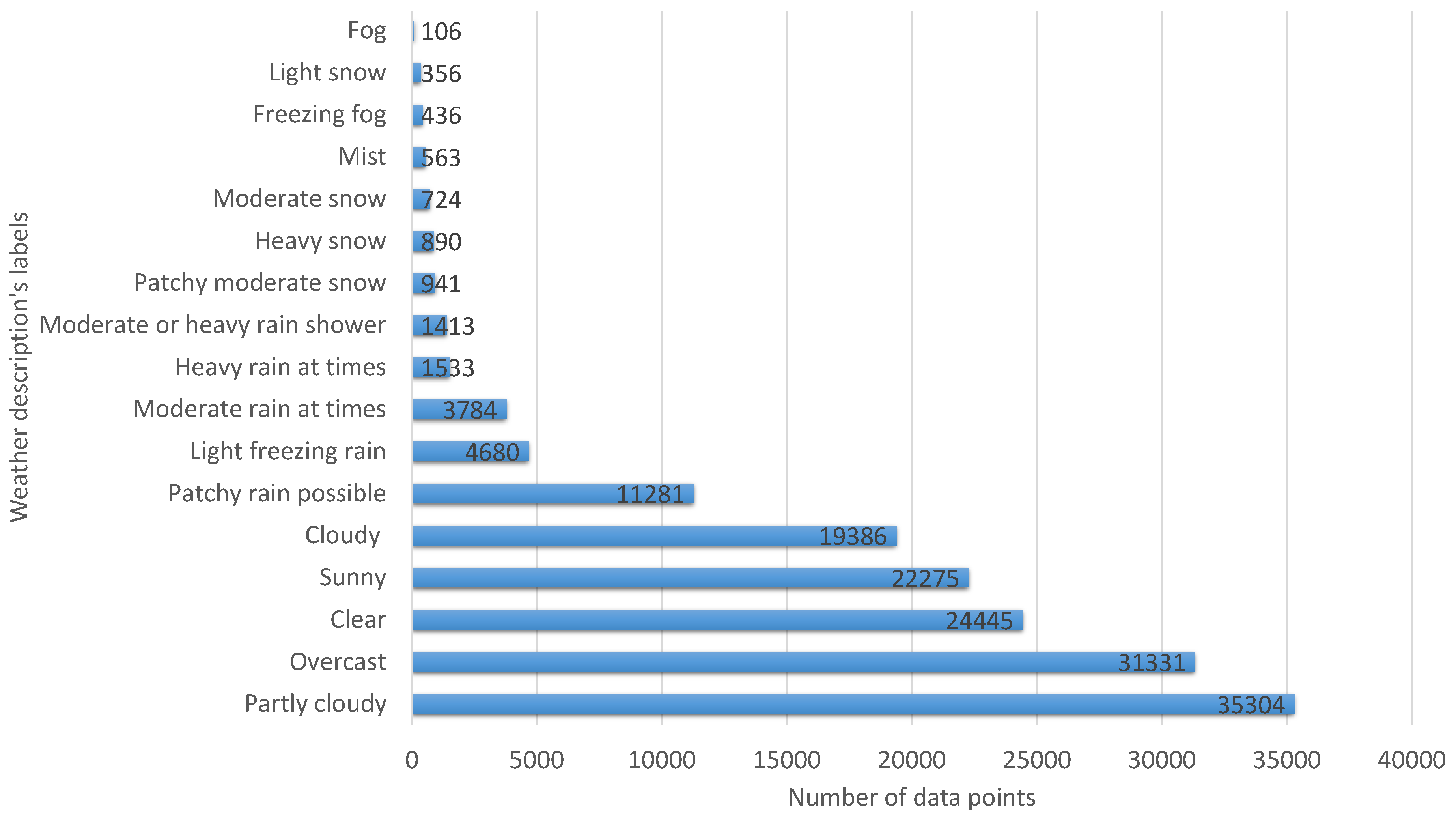
shows the input features of some entries in the first dataset. Figure 4 displays a histogram representing the distribution of weather conditions (weather descriptions) in the first dataset, spanning 13 years. The weather conditions serve as the labels used to train the models. From the figure, which is ordered from the highest to the lowest number of occurrences, it is observed that partly cloudy weather occurs most frequently, with 35,304 samples, followed closely by overcast, with 31,331 samples, and clear, with 24,445 samples. On the other hand, fog occurs the least frequently in the dataset, with only 106 samples.

5. Experimental Setup, Results, and Discussion

In the datasets, some input and output features encompass nominal values that are not readily usable for the training of models. These categorical data need to be transformed into numerical representations to facilitate processing. Hence, we applied an encoding strategy to convert these nominal values into corresponding numerical values. Following the model’s output generation, decoding was introduced to revert these numerical predictions to their original nominal forms. Additionally, duplicated entries within the datasets were identified and eliminated during the data preparation phase to maintain data integrity and prevent overfitting.

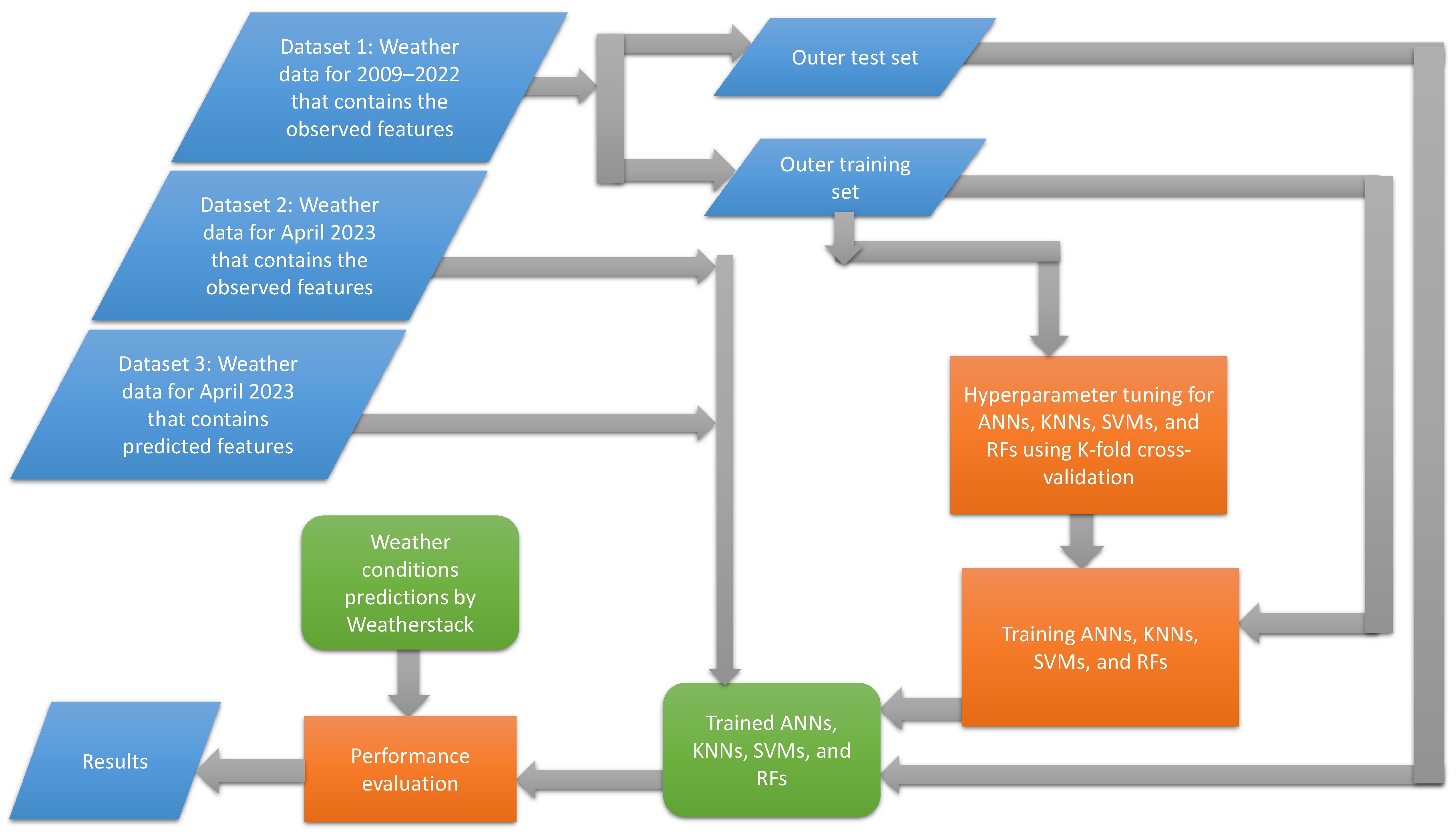
This section presents an assessment and comparison of the performance of ANNs, KNN, RF, and SVMs in weather forecasting. As demonstrated in Figure 5, our evaluation process consisted of several steps. Firstly, we partitioned the collected dataset 1, comprising weather data from 2009 to 2022, into an outer training set and an outer test set. An outer training set plays a dual role: it assists in fine-tuning the hyperparameters of each method and is also used to train the models with the optimized hyperparameters. Then, the performance of the trained models was evaluated using three separate sets of data: the outer test set, dataset 2, containing observed weather data for April 2023; and dataset 3, containing predicted features for April 2023. Evaluating the models using three distinct datasets enhanced the reliability and accuracy of the results, providing a robust understanding of each model’s forecasting capabilities. In this study, Weatherstack was used not only as a source of weather data but also to benchmark the performance of our developed models. Weatherstack has its own model for the classification of weather conditions. By benchmarking our models’ predictions against those from Weatherstack, the validity and effectiveness of our developed models could be assessed in the context of real-world, industry-standard predictions.

The hyperparameters were optimized using a k-fold cross-validation scheme integrated with grid search. This process is essential as the performance of learning models depends significantly on the optimal selection of the hyperparameters. During the k-fold cross-validation process, the outer training set is partitioned into k exclusive folds. The model is then trained using k-1 folds, while the remaining folds serve as the validation set to evaluate the model’s predictive performance. This process is repeated such that each fold is used exactly once for validation. Subsequently, the hyperparameter values that yield the highest average classification accuracy across all folds are selected as the optimal parameters for the learning models [21]. This approach ensured that our models were trained using robust, scientifically sound practices that enhanced their performance and predictive accuracy. In this study, the number of folds was set to 5. Regarding the train, test, and validation split, we used 80% for training, 10% for the test, and 10% for validation.

The experiments were conducted utilizing Python [22], a powerful and versatile programming language widely adopted in machine learning and data analysis. Various open-source libraries were also employed to assist in the experimental process: NumPy [23] and Pandas [24] for data manipulation, Matplotlib [25] and Seaborn [26] for data visualization, Scikit-learn [27] for machine learning algorithms, and TensorBoard, TensorFlow [28], and Keras [29] to create and manage neural networks. Each library provides specialized functions that facilitate various aspects of data analysis and machine learning model development [30]. The accessibility of Google Colab, an online runtime environment for data analysis, also contributed to the efficient development of the models.

5.1. ANNs

Feedforward neural networks consist of several layers of neurons, which process the input data and pass them forward until a prediction is made at the output layer. The networks have both parameters and hyperparameters that influence their performance. The parameters in feedforward neural networks are the weights and biases that the model learns during training to make accurate predictions. Hyperparameters, on the other hand, are configuration variables set before training, such as the number of hidden layers and neurons in the network, the learning rate, and the choice of activation and loss functions. The number of hidden layers and neurons in each layer impacts the model’s complexity and its ability to learn diverse data patterns. The learning rate controls how rapidly the model learns. The choice of activation and loss functions influences how the model handles nonlinearities and measures prediction errors, respectively. All these hyperparameters collectively shape the model’s learning efficiency and overall performance.

The number of hidden layers and neurons, as the most important hyperparameters in ANNs, were optimized using 5-fold cross-validation. More specifically, a systematic search was performed over multiple combinations of hidden layers and neurons, and the combination delivering the highest average cross-validated accuracy was selected as the optimal choice.

Table 2. Results of cross-validation to find the best-performing ANN model by tuning the number of neurons in the first hidden layer and the number of neurons in the second hidden layer as hyperparameters.

Number of Neurons in the First Hidden Layer	Number of Neurons in the Second Hidden Layer	Validation Accuracy (%)
33	33	95.37
33	34	95.51
33	35	95.58
33	36	95.37
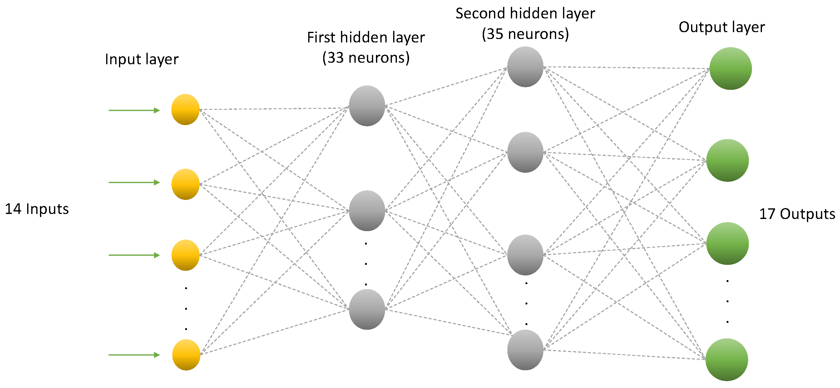
33	37	95.39

shows the cross-validated accuracy of some of the combinations close to the optimal combination. As demonstrated in the table, the best setup was found to have 33 neurons in the first hidden layer and 35 neurons in the second hidden layer. Figure 6 shows the architecture of the implemented ANN.

The SoftMax activation function is used in the output layer as this is a multi-class classification problem, and it returns the probabilities of each class. The model uses the rectified linear unit (ReLU) activation function in the hidden layers. The ReLU activation function is defined as follows [31]:

$$f\left(x\right)=max(0,x)$$

(5)

where x is the input to the function. The ReLU function sets any negative values in the input to zero and leaves positive values unchanged. The ReLU function is popular in neural networks because it is computationally efficient and helps to prevent the vanishing gradient problem that can occur with other activation functions. The vanishing gradient problem occurs when the gradient of the loss function with respect to the weights becomes very small, making it difficult for the network to learn [32]. A batch normalization layer was also incorporated into the network, serving to normalize the inputs of each layer. It allows faster learning and higher overall accuracy [33].

To adjust the weights and biases in the network, the Adam optimizer was used [34]. It is a widely employed method that distinguishes itself by dynamically adjusting the learning rate for different parameters. This ensures that each parameter is updated at a rate specifically tailored to its behavior, leading to improved convergence and stability during training. Additionally, it incorporates the concept of momentum by adding a fraction of the previous update to the current one, hence reducing oscillations and accelerating the training process. With its ability to automatically adjust the learning rate and speed up training, Adam is an appealing choice. It not only minimizes the time required for training but also reduces the need for extensive manual tuning of the hyperparameters.

In training, the loss function was set to categorical cross-entropy, the maximum number of training epochs was set to 50, the batch size was set to 800, and the initial learning rate was set to 0.002. Early stopping was also used to prevent the risk of model overfitting during the training phase [35]. Overfitting refers to a situation whereby a model, due to its excessive complexity, aligns too closely to the training data, thereby compromising its ability to perform accurately on new, unseen data. By using early stopping, the training process is terminated once the model’s accuracy for validation data no longer improves, ensuring its robustness and generalization capacity [36,37].

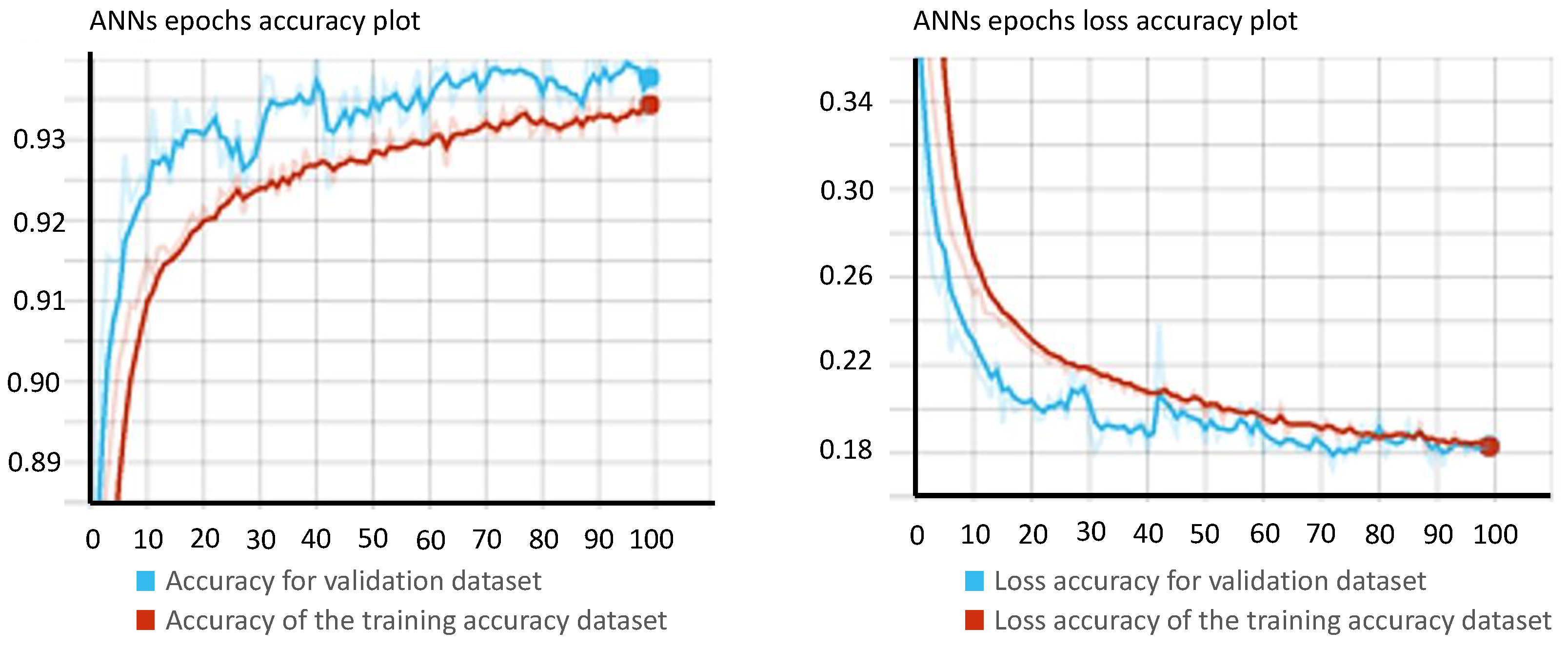
Moreover, to monitor the training progress and evaluate the model’s performance during training, the epoch loss function and epoch accuracy were used. The epoch loss function measures the difference between the predicted output and the actual output during one epoch of training, while the epoch accuracy measures the percentage of correctly classified samples in the training dataset. In Figure 7, the epoch loss and epoch accuracy are plotted against the number of epochs. The blue line represents the training accuracy and loss for the model. On the other hand, the red line represents the validation accuracy and loss for the model. These two metrics are critical in assessing the performance of a model and determining when to stop the training to avoid overfitting. The performance of the final trained ANN model was evaluated on the outer test set, yielding remarkable accuracy of 97.00%.

5.2. RF

RF is an ensemble learning method that generates a collection of decision trees for predictive modeling [17]. Each decision tree is constructed using a random subset of the input features and training samples. This randomness contributes to the creation of an ensemble of diverse decision trees that capture different patterns in the data [38]. The final prediction of the RF model is determined by aggregating the predictions of the individual trees, typically via majority voting. This ensemble approach significantly enhances the model’s robustness, reducing overfitting and improving its generalization to unseen data [39].

In building and optimizing RF models, several key hyperparameters are important, including the number of trees (estimators), the maximum depth of trees, the maximum number of features, and the splitting criterion. The number of trees specifies the count of decision trees in the forest, influencing the robustness and computational demand of the model. Increasing the number of estimators typically improves the model’s accuracy but also increases the computational complexity [40]. The maximum depth of trees defines the longest path from the root to a leaf, thereby controlling model complexity and preventing overfitting. A deeper tree can better capture complex relationships in the data but is also more prone to overfitting. The maximum number of features determines the subset of features considered at each split, offering control over the model’s randomness and bias–variance balance. Finally, the splitting criterion measures the effectiveness of a split within a tree, thereby influencing the decision-making mechanism in each tree.

The number of estimators and the maximum depth of trees were fine-tuned using a grid search approach in combination with 5-fold cross-validation. Using this approach, different combinations of the number of trees and the maximum depth were tested, and the configuration that resulted in the best cross-validation performance was selected.

Table 3. Results of cross-validation to find the best-performing RF model by tuning the number of estimators and the maximum depth of the tree as hyperparameters.

Number of Estimators	Maximum Depth of Trees	Validation Accuracy (%)
195	25	95.75
196	25	95.71
197	25	95.73
198	25	95.70
199	25	95.73
200	25	95.70

provides a detailed overview of the cross-validated accuracy for a number of combinations in close proximity to the optimal one. As the table shows, the optimal number of estimators and the maximum depth of trees are 195 and 25, respectively.

Moreover, the Gini index was used as the splitting criterion. It measures the probability of incorrectly classifying a randomly chosen sample from the dataset [41]. The Gini impurity equation is defined as follows [42]:

$$Gini=1-\sum _i{p}_i(1-p_i)$$

(6)

where i is the index of each class in the dataset, and $p_i$ is the proportion of samples belonging to class i in the dataset. The Gini index was used due to its computational efficiency and tendency to favor multi-class splits, making it well suited to our problem. Furthermore, its calculation does not involve logarithmic functions, enabling faster model training without compromising the accuracy of the results. The maximum number of features was also set to 14, the total number of features in the dataset. After selecting the hyperparameters, we initialized the RF classifier model and trained it using the outer training set. Upon testing the trained RF model on the outer test set, we attained an accuracy score of 96.69%.

5.3. KNN

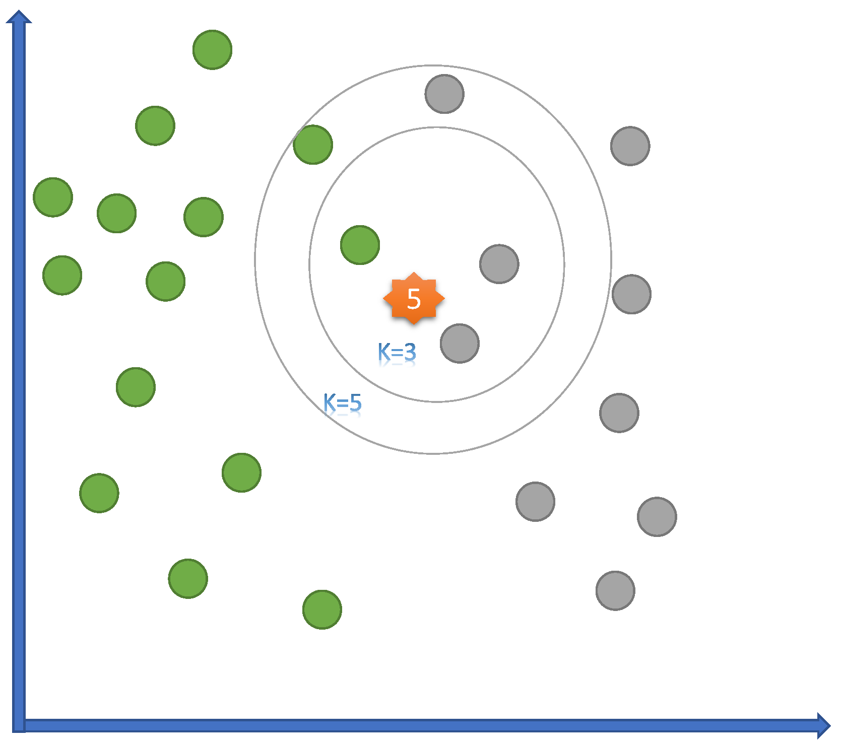
KNN is a simple but effective algorithm for classification that works by identifying the k closest data points to the input and assigning the input to the most common class among these k neighbors. The number of neighbors k is the most critical hyperparameter for KNN. It represents the number of neighbors that the algorithm examines in order to predict. A small value of k means that noise will have a greater influence on the result, while a large value makes it computationally expensive. The number of neighbors k was tuned using a grid search approach in combination with 5-fold cross-validation.

Table 4. Results of cross-validation to find the best-performing KNN model by tuning the number of neighbors (k).

Number of Neighbors (k)	Validation Accuracy (%)
1	76.01
3	76.78
5	77.64
7	76.55
9	76.46

shows the cross-validation accuracy for some values of hyperparameter k. The table illustrates that the optimal value for k appears to be 5, which yields the highest cross-validation accuracy. Therefore, this value was selected to perform predictions on the test sets. Moreover, the distance metric was set to Euclidean, and all points in the neighborhood were weighted equally to predict the output. Given the high dimensionality of our dataset, we employed an exhaustive search method to ensure that k closest neighbors were accurately identified. The trained KNN model was tested on the outer test set, and the accuracy was 77.97%. Firstly, this might be a reflection of the robust nature of our dataset. If our data instances are well clustered, then a slight variation in the number of neighbors would not significantly affect the model’s ability to correctly classify instances, as the majority of the neighbors would still belong to the correct class. Second, it might also suggest that our data have a lower degree of noise. In noisier datasets, the choice of the number of neighbors can have a more noticeable impact, as fewer neighbors can lead to overfitting to the noise, while more neighbors can help to smooth out the noise.

5.4. SVMs

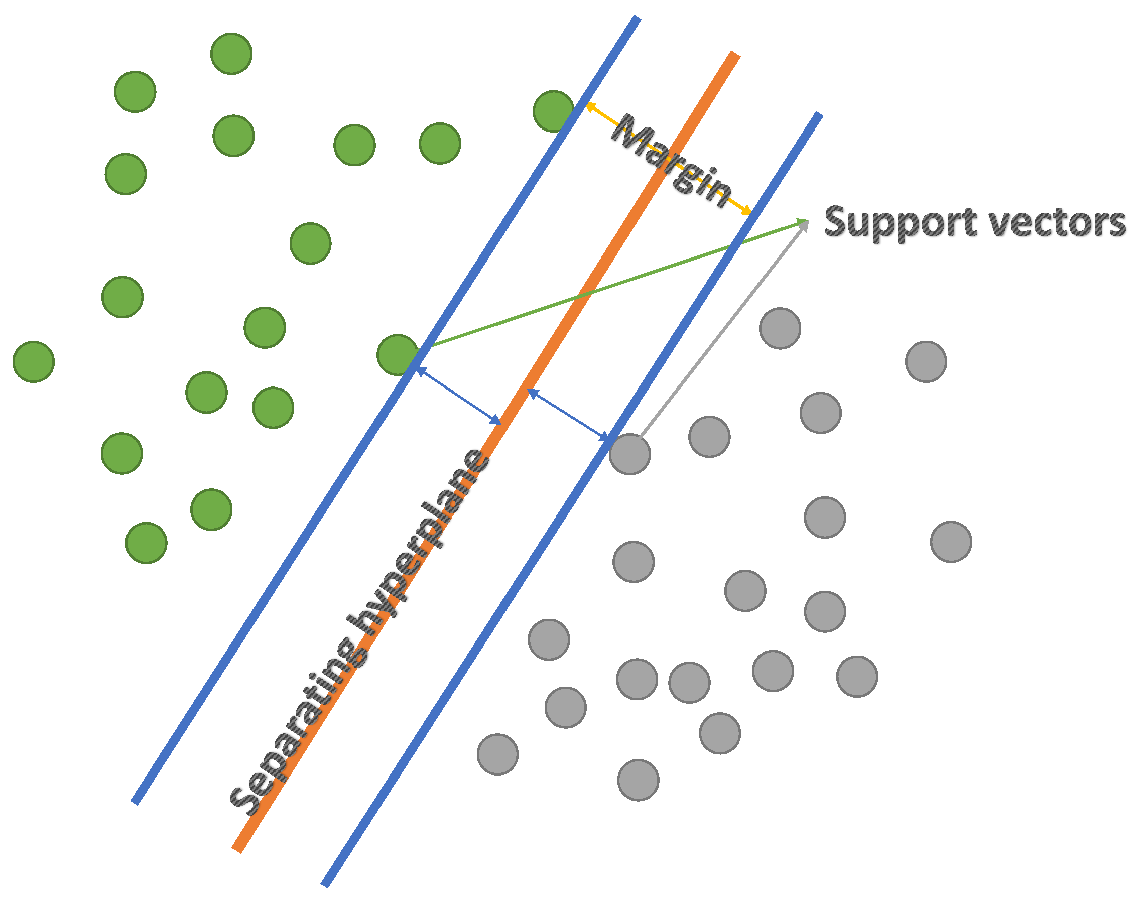
SVMs seek a maximum-margin hyperplane as a decision boundary, aiming for the most substantial possible separation between different classes. This strategy makes SVMs reliable and precise in their classification performance. The use of the RBF kernel in SVMs further contributes to this precision. The RBF kernel allows SVMs to handle complex, nonlinear, and high-dimensional data, making it a preferred choice over linear kernels in many cases. It essentially maps the input space into a higher-dimensional feature space, ensuring that the data are more likely to be linearly separable.

However, the efficient performance of SVMs strongly relies on fine-tuning two pivotal hyperparameters—the box constraint and the kernel scale. The box constraint balances the model’s complexity against its capacity to tolerate errors. A higher box constraint can lead to a precise but potentially overfitted model, whereas a lower value can cause the model to oversimplify, risking underfitting. The kernel scale adjusts the shape of the decision boundary. High kernel scale values produce a more rigid boundary, which may lead to underfitting. Conversely, low kernel scale values allow for more flexible boundaries, which can capture intricate data patterns but may also risk overfitting. Thus, tuning these hyperparameters properly is essential to achieve the desired bias–variance trade-off and optimal model performance.

Similar to the previous methods, the hyperparameters—the box constraint and the kernel scale—were fine-tuned using a grid search approach in combination with 5-fold cross-validation.

Table 5. Results of cross-validation to find the best-performing SVM model by tuning the box constraint and kernel scale ($\gamma$).

Box Constraint	Kernel Scale ($\mathit{\gamma }$)	Validation Accuracy (%)
1.00	0.10	93.02
1.00	1.00	87.45
10.00	0.10	95.44
10.00	1.00	88.33

shows the cross-validated accuracy for some of the best combinations. As the table shows, the optimal values for the box constraint and the kernel scale are 10 and 0.1, respectively. After training, the obtained trained SVM model was evaluated on the outer test set, resulting in remarkable accuracy of 93.00%.

5.5. Comparing the Performance of the Methods

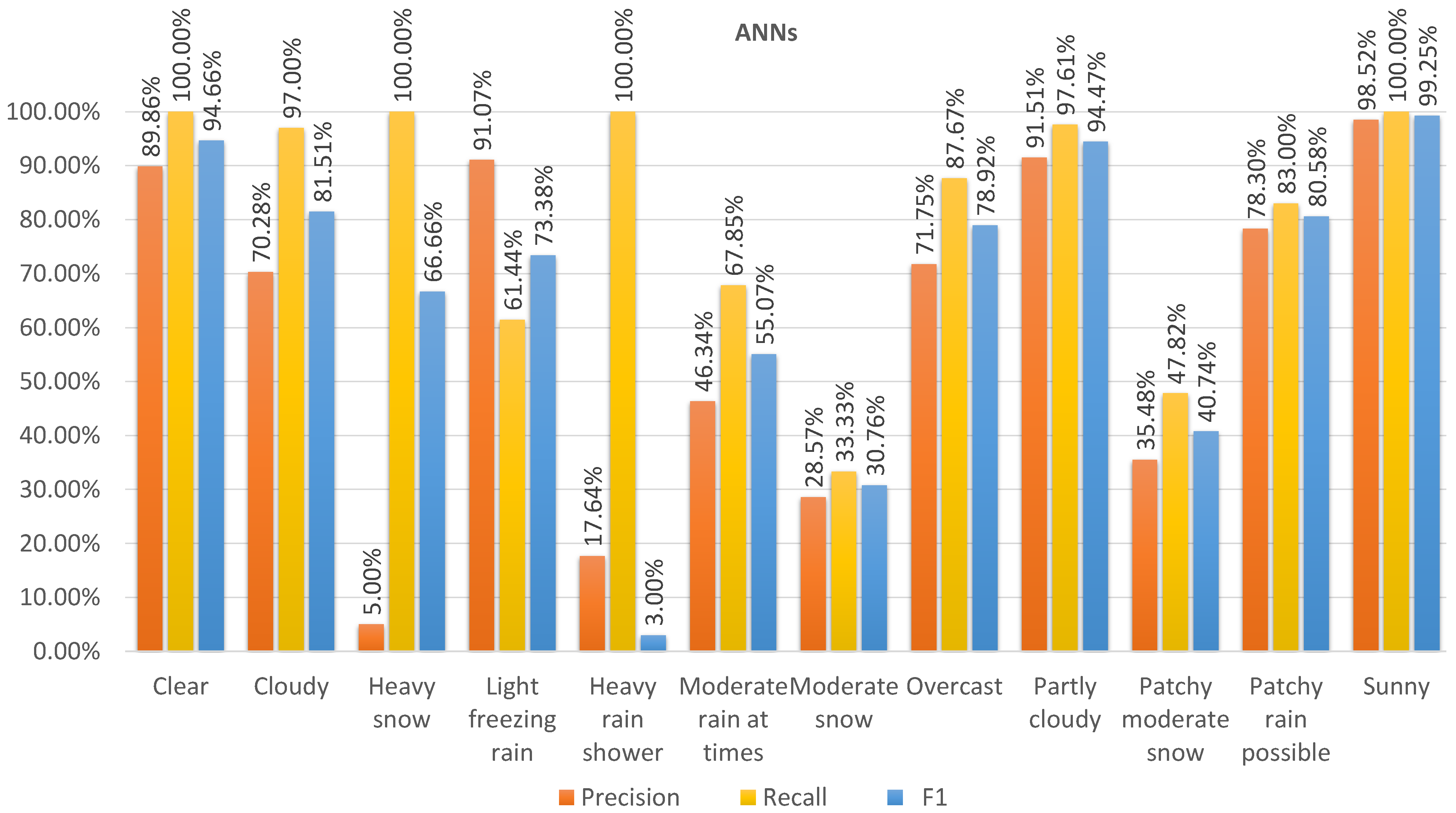
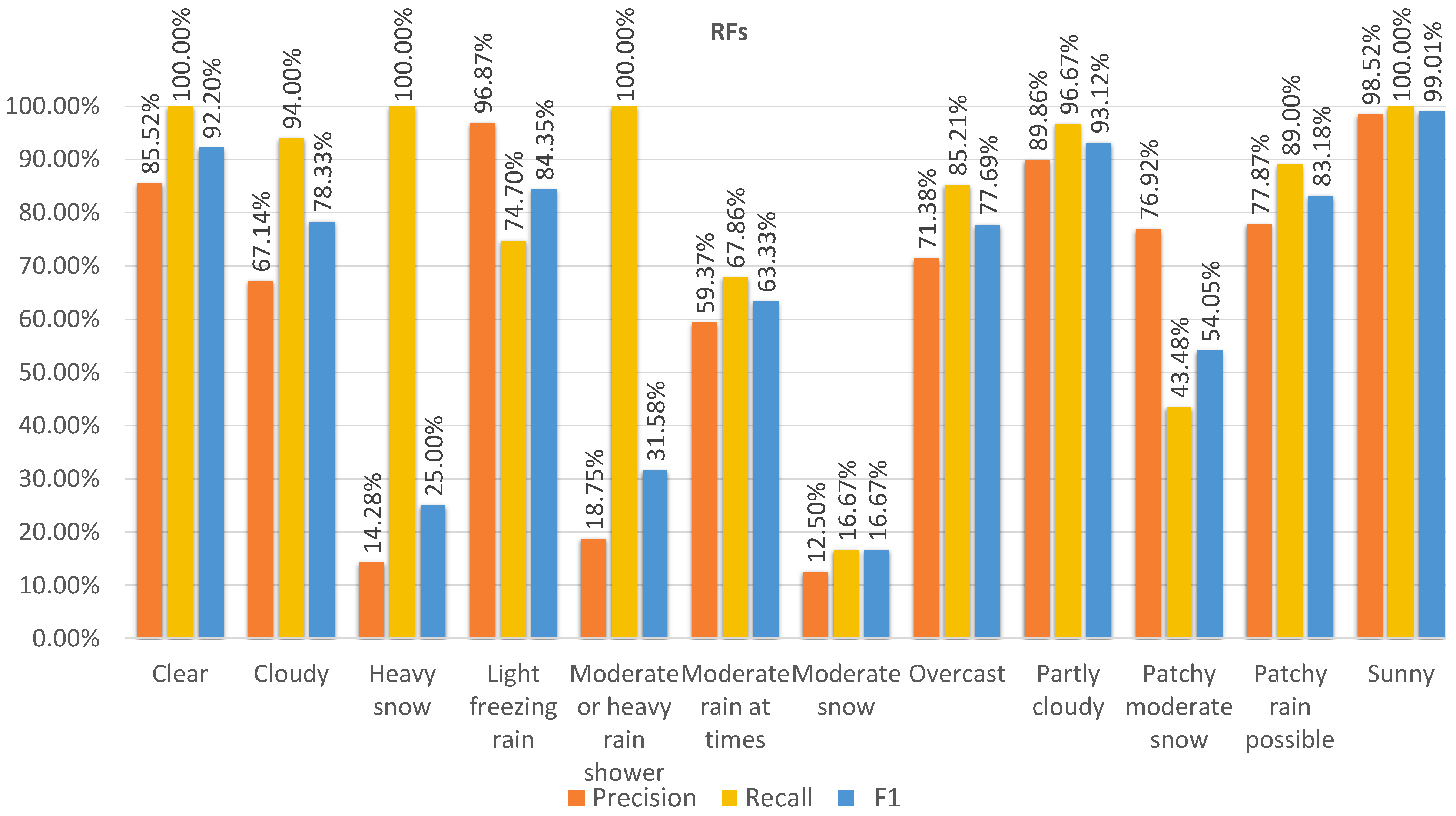
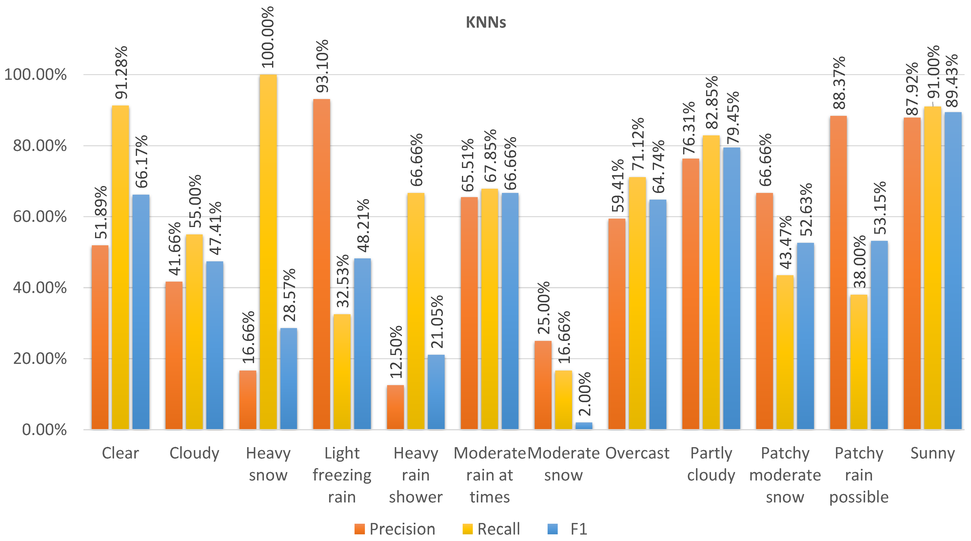
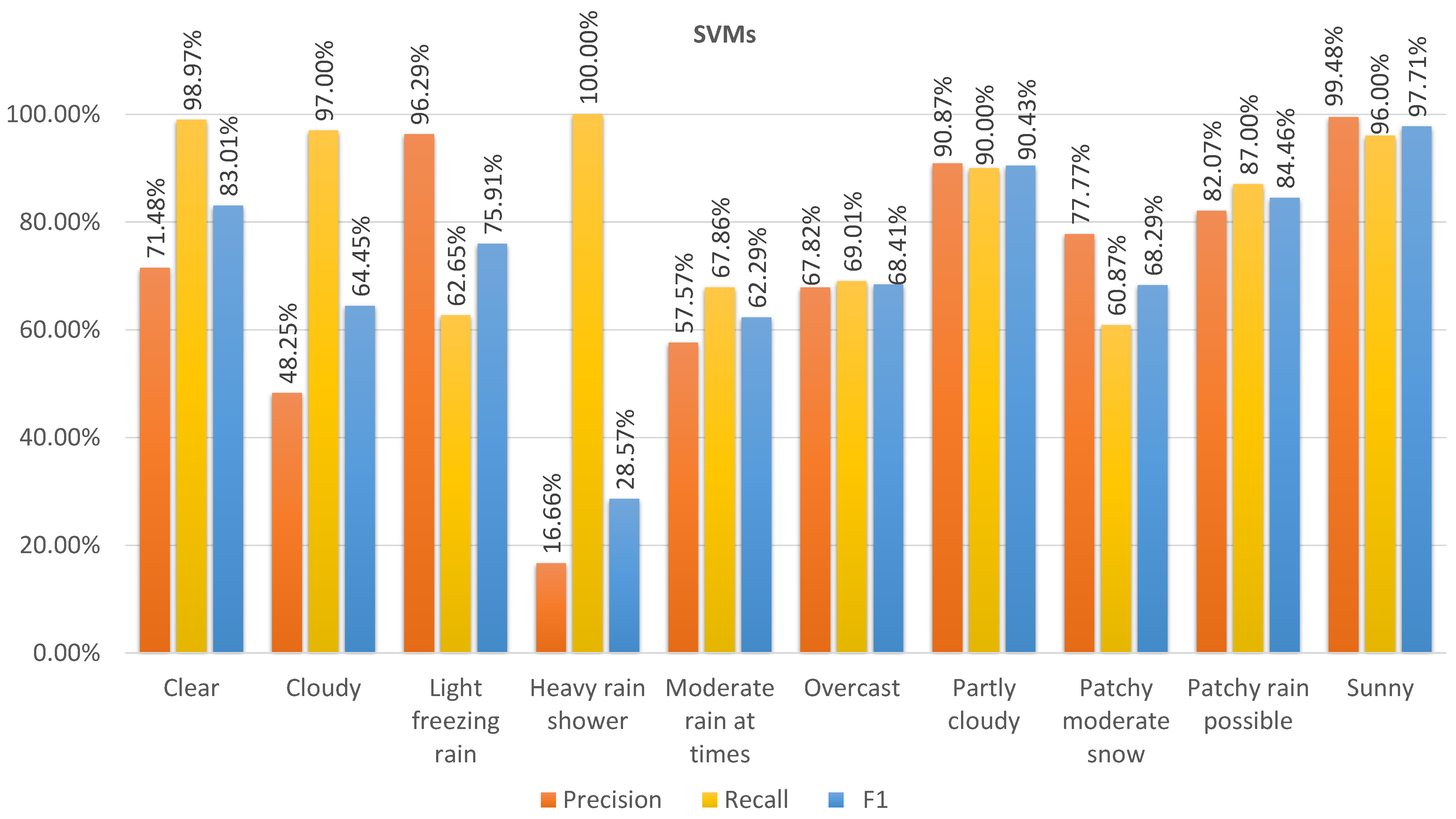
In this section, we compare the performance of the developed models based on SVMs, ANNs, KNN, and RF and benchmark them against the performance of Weatherstack. Figure 8, Figure 9, Figure 10 and Figure 11 show the precision, recall, and F1 scores for the different classes predicted by the models on dataset 2. The ANN achieved the highest F1 score in the majority of classes, indicating a good balance between precision and recall. RF had slightly lower F1 scores than the ANN but performed better than KNN and SVM, which had the lowest F1 scores. Regarding recall, KNN maintained the highest score, while the ANN and RF showed comparable performance. Moreover, the SVM had the lowest recall score. In terms of precision, RF achieved the highest score, and the ANN closely followed, with similar performance. On the other hand, the KNN and SVM had lower precision scores.

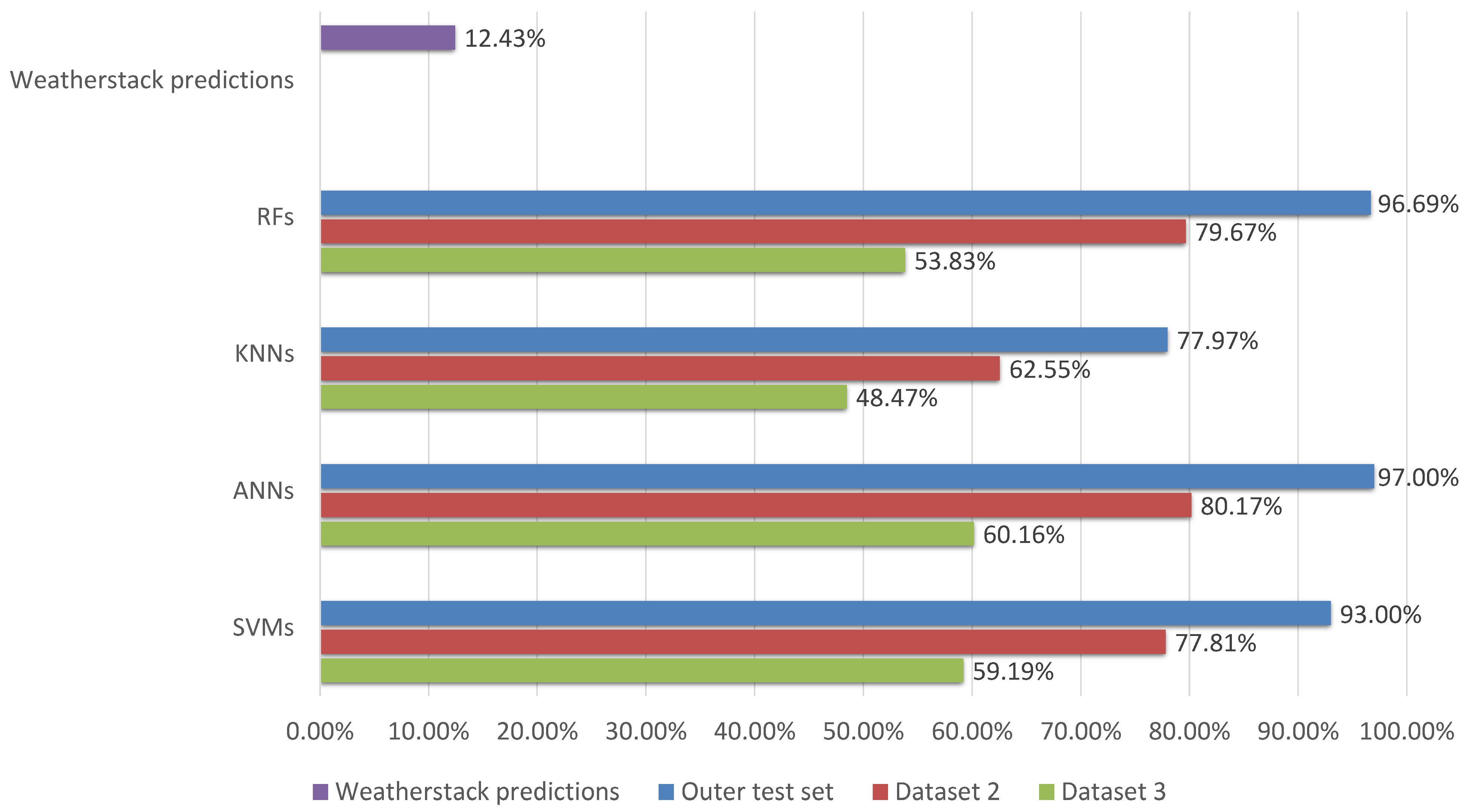
Figure 12 compares the performance of each developed model on the outer test set, dataset 2, and dataset 3 in terms of the accuracy score. In this figure, the y-axis represents the model name, while the x-axis represents the accuracy percentage. For dataset 2, the ANN has the highest accuracy, with a value of 80.17%. The RF also performs well, with accuracy of 79.67%. The SVM and KNN have the lowest accuracy rates, with 77.81% and 62.55%, respectively. For dataset 3, the ANN has the highest accuracy, with a value of 60.16%. The SVM also performs well, with accuracy of 59.19%. RF and KNN have the lowest accuracy rates, with 53.83% and 48.47%. Overall, the results suggest that the ANN model is the most accurate model in predicting weather conditions in all datasets. The performance of the developed models was also benchmarked against the performance of the Weatherstack model. As is evident from the figure, the accuracy of Weatherstack’s model is 12.43%, highlighting the substantial performance advantage of our developed models over Weatherstack’s model. ANNs have an inherent capacity for feature learning, allowing them to construct higher-level features from the raw input data, which likely contributed to their enhanced performance in our study. SVMs, RF, and KNN rely on manual feature extraction, which might not always capture the necessary information for accurate weather forecasting.

It can be observed from the figure that the models demonstrate a lower level of accuracy on dataset 2 compared to the outer test set. This might be attributed to several factors, such as temporal differences and distribution shifts. More specifically, the weather patterns in dataset 2, which corresponds to April 2023, might differ from the patterns in the original training data that span 2009 to 2022 due to climate change. Additionally, the statistical properties of the April 2023 data could differ from those of the original dataset, meaning that the models are less effective at predicting these new patterns.

The figure further shows that the models yield even lower accuracy on dataset 3 in comparison to both the outer test set and dataset 2. This decrease may result from the nature of the input features within dataset 3. Unlike the previous datasets, dataset 3 consists of predicted rather than observed input features for April 2023. These predicted features are subject to a level of uncertainty and possible prediction errors that could have been introduced during their generation by Weatherstack. Furthermore, potential mismatches between the predicted and true values, or differences in their respective statistical distributions, can lead to poorer model performance when applied to such data.

6. Conclusions and Future Work

In this study, we developed and evaluated four models based on ANNs, SVMs, RF, and KNN for the classification of weather conditions for multiple cities in Sweden. The results indicated that the trained ANN model had the best performance on all the employed datasets in comparison to other machine learning models. We also benchmarked our models with the model of Weatherstack, and the results showed that all four developed models significantly outperformed the model of Weatherstack, suggesting that machine learning techniques can be highly effective in classifying weather conditions and that the choice of model can significantly impact the prediction accuracy. Moreover, our results illuminated the consequential impact of the model choice on the prediction accuracy and the vital role of hyperparameter optimization in achieving the best performance.

The study also revealed interesting variations in model performance across different datasets. The accuracy on the test set, comprising observed data from 2009 to 2022, was notably higher than on dataset 2 and dataset 3, both representing April 2023. This variance emphasizes the influence of temporal differences and possible distribution shifts on model performance. Moreover, the disparity was more pronounced on dataset 3, which contained predicted rather than observed input features, highlighting the potential complexities introduced by the inherent uncertainty and possible prediction errors within such data. These insights provide a foundation for future research and development in enhancing model adaptability and robustness across varied data scenarios.

In light of the findings of this study, there are several potential avenues to enhance the accuracy of future research. One suggestion is to augment the existing 14 features of the input data with the date as an additional attribute. By incorporating the date, it would be possible to encode temporal patterns and trends, which may improve the predictive accuracy of the model. Additionally, future work could benefit from adopting instance selection methods. Such methods aim to filter out noisy data or outliers from the training dataset, thus refining the classifier’s ability to distinguish between different classes in the testing dataset. Techniques such as data reduction based on locality-sensitive hashing (DRLSH) [43] and border point extraction based on locality-sensitive hashing (BPLSH) [44] have been demonstrated as effective in this regard. AdaBoost [45] and XGBoost [46] are interesting models that can be used for comparisons in future work on weather predictions, as they have demonstrated good performance in categorizing data. XGBoost is particularly intriguing due to its emphasis on speed and high accuracy, making it suitable for scenarios where these factors are crucial. On the other hand, AdaBoost is known to work best in datasets with minimal noise.