
Seasonal Distribution and Source Apportionment of Chemical Compositions in PM2.5 in Nanchang, Inland Area of East China
 ,
,
Abstract
:1. Introduction
2. Materials and Methods
2.1. Sample Collection
2.2. Determination of PM2.5 and Its Chemical Components
2.3. Date of Meteorological Factors
3. Results and Discussion
3.1. Distribution Characteristics of Different Components of PM2.5
3.1.1. Proportion of Components of PM2.5 and Its Seasonal Distribution
3.1.2. Distribution of OC and EC
Distribution of OC
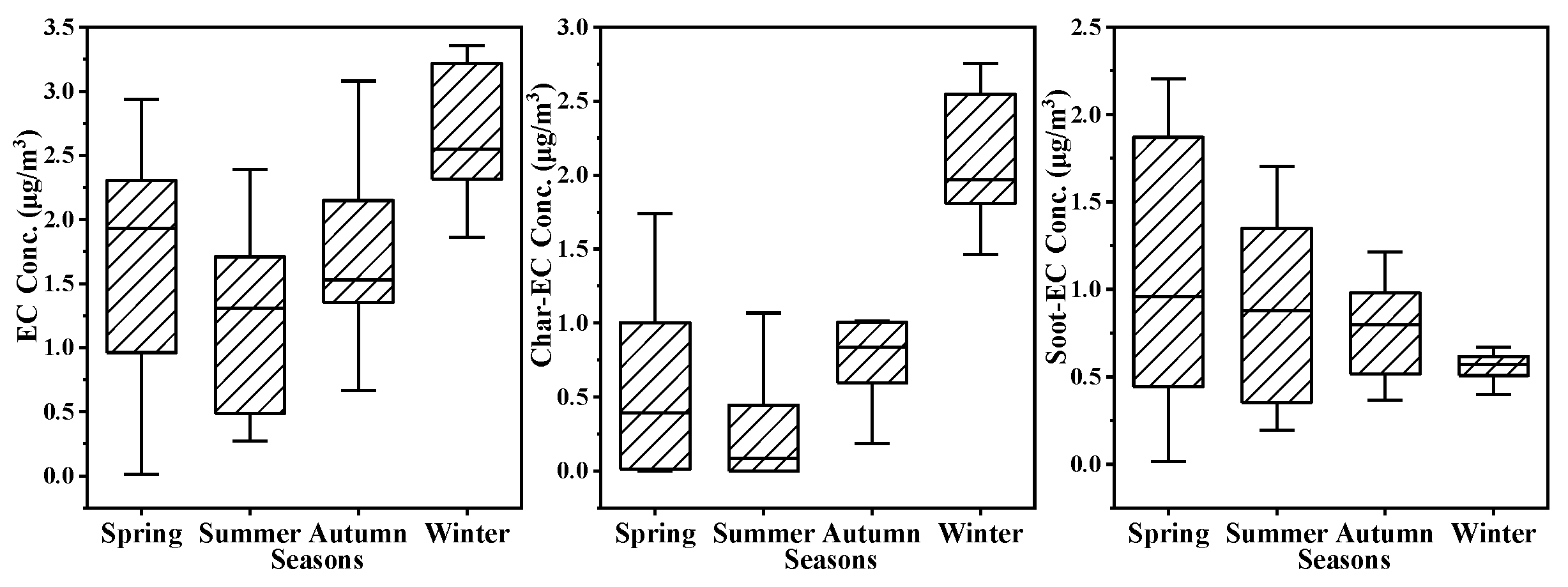
Distribution of EC
Comparison of OC and EC in This Study with Those in Other Cities
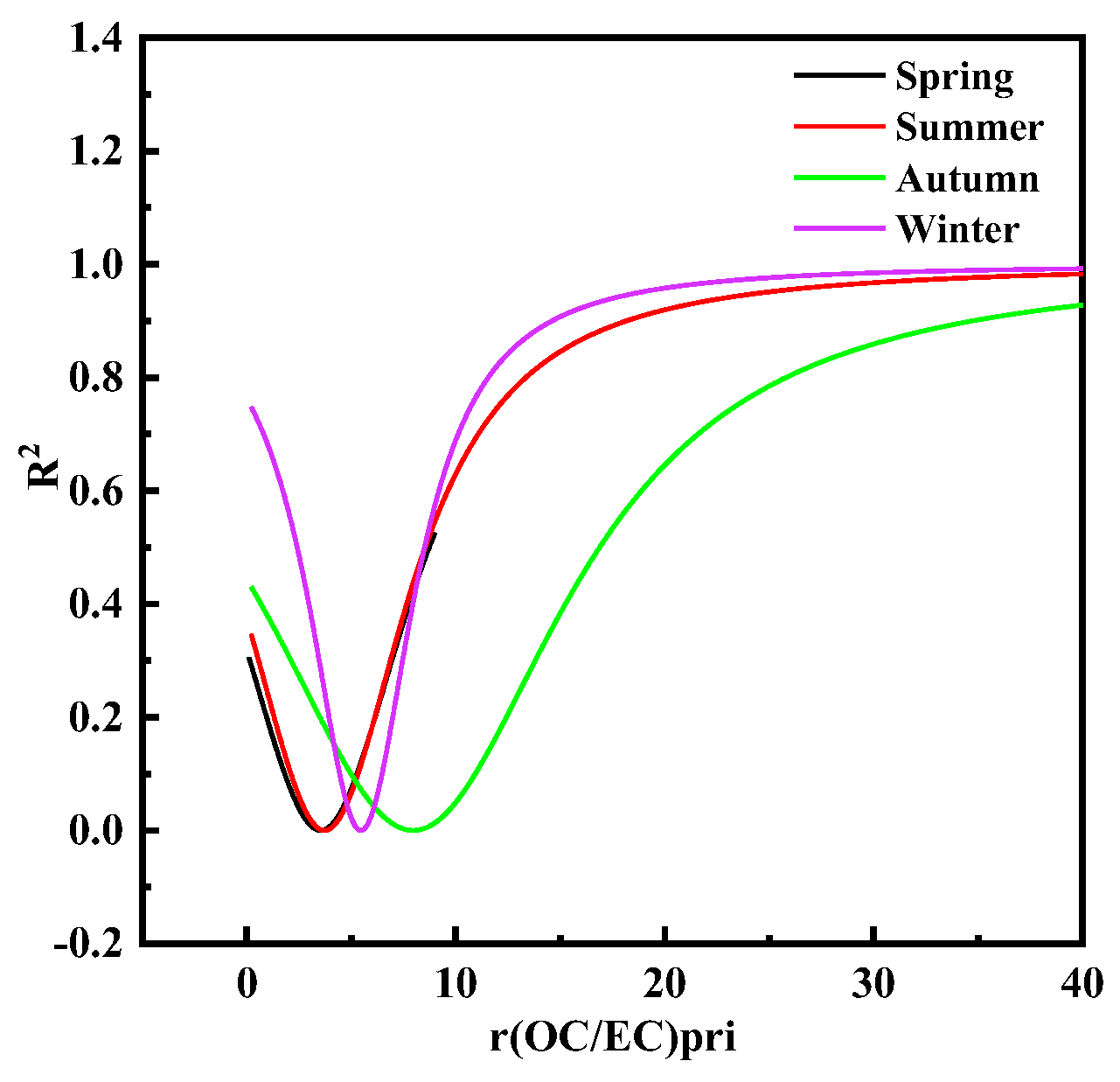
3.1.3. Distribution of SOC
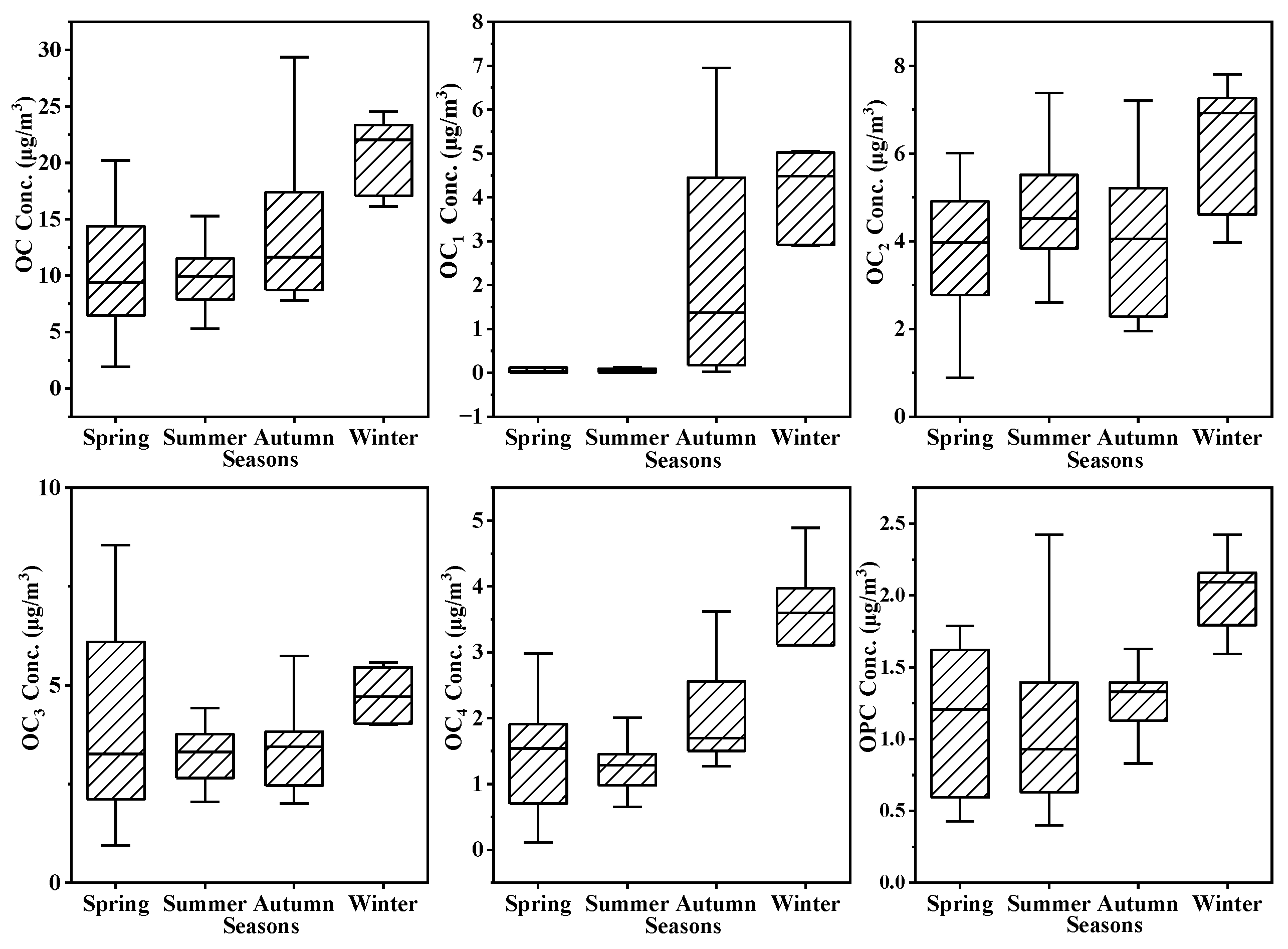
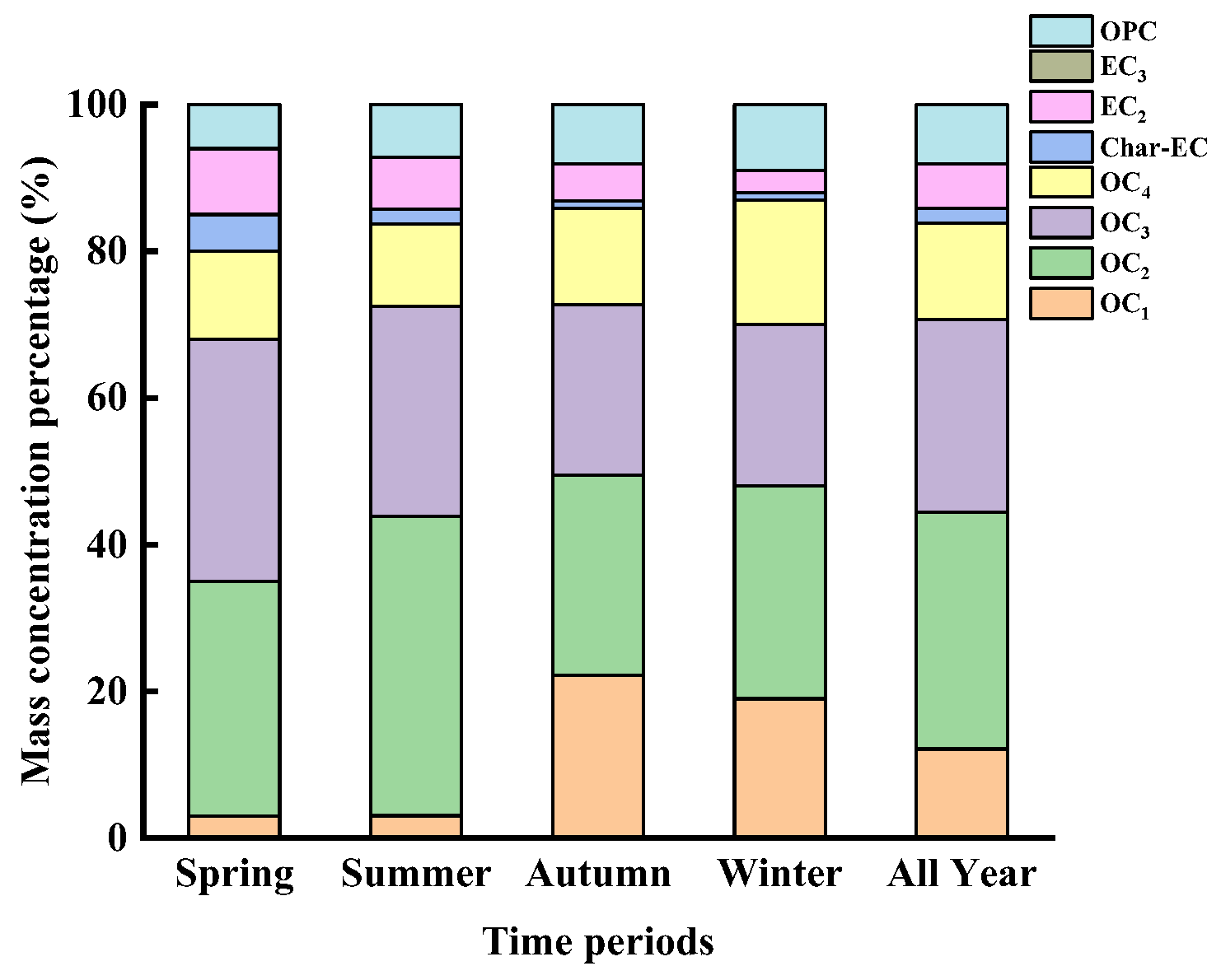
3.1.4. Distribution of Eight Carbon Fractions
3.1.5. Distribution of Water-Soluble Ions
3.2. Source Apportionment of PM2.5
3.2.1. Source-Analysis Based on the Correlations between Chemical Compositions
Correlations between OC and EC
Correlations between Water-Soluble Ions
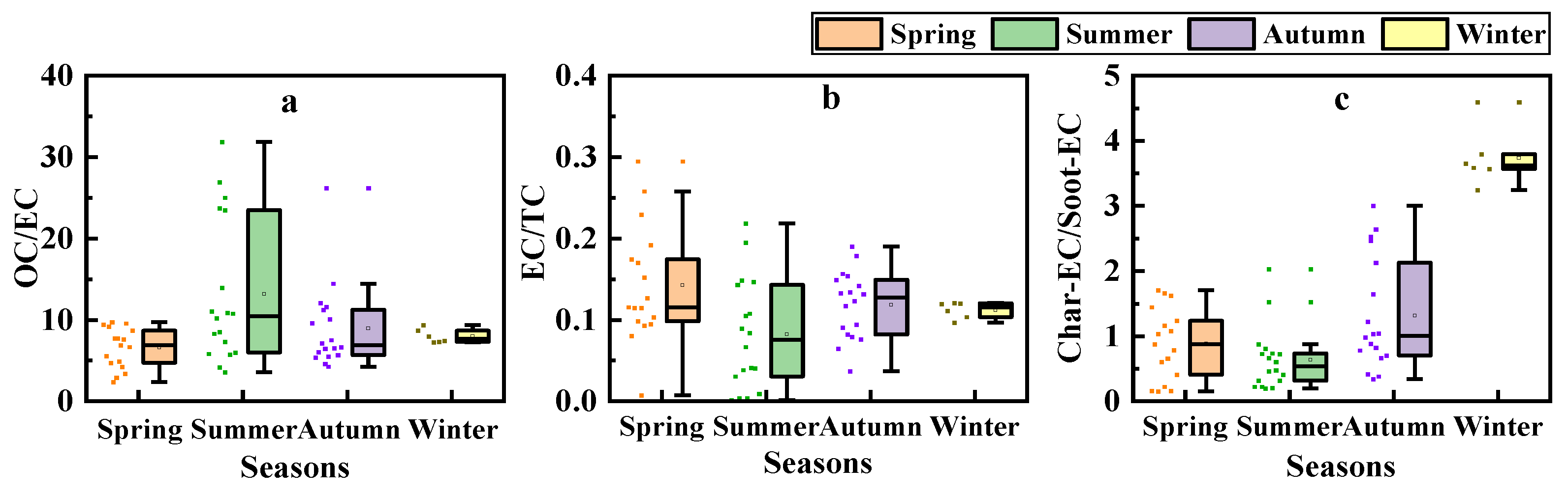
3.2.2. Source-Analysis Based on OC/EC, EC/TC, and Char/Soot
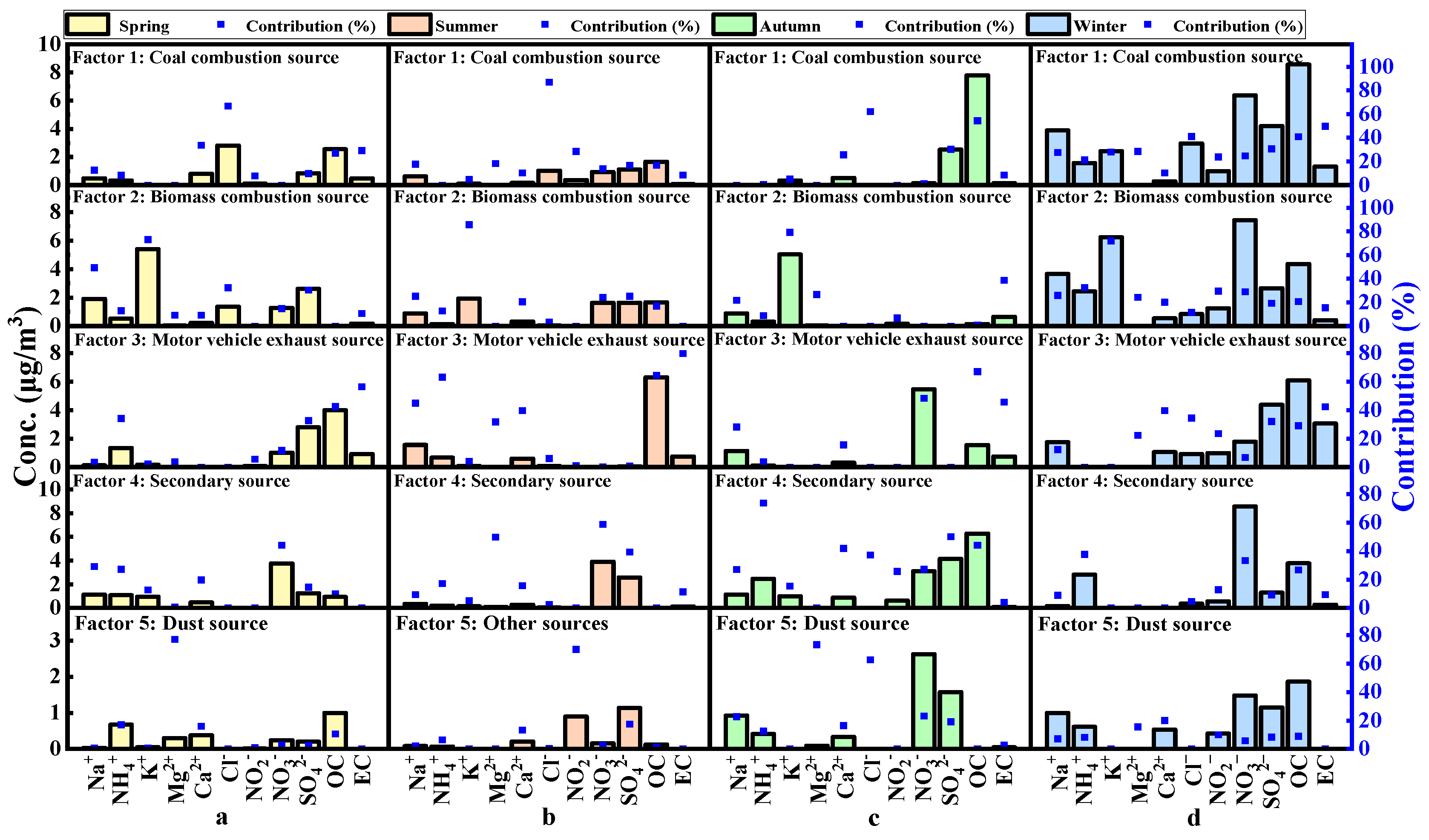
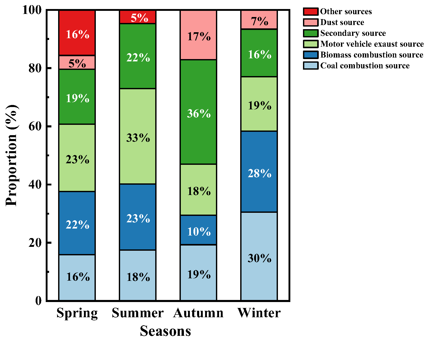
3.2.3. Source-Analysis Based on the PMF Method
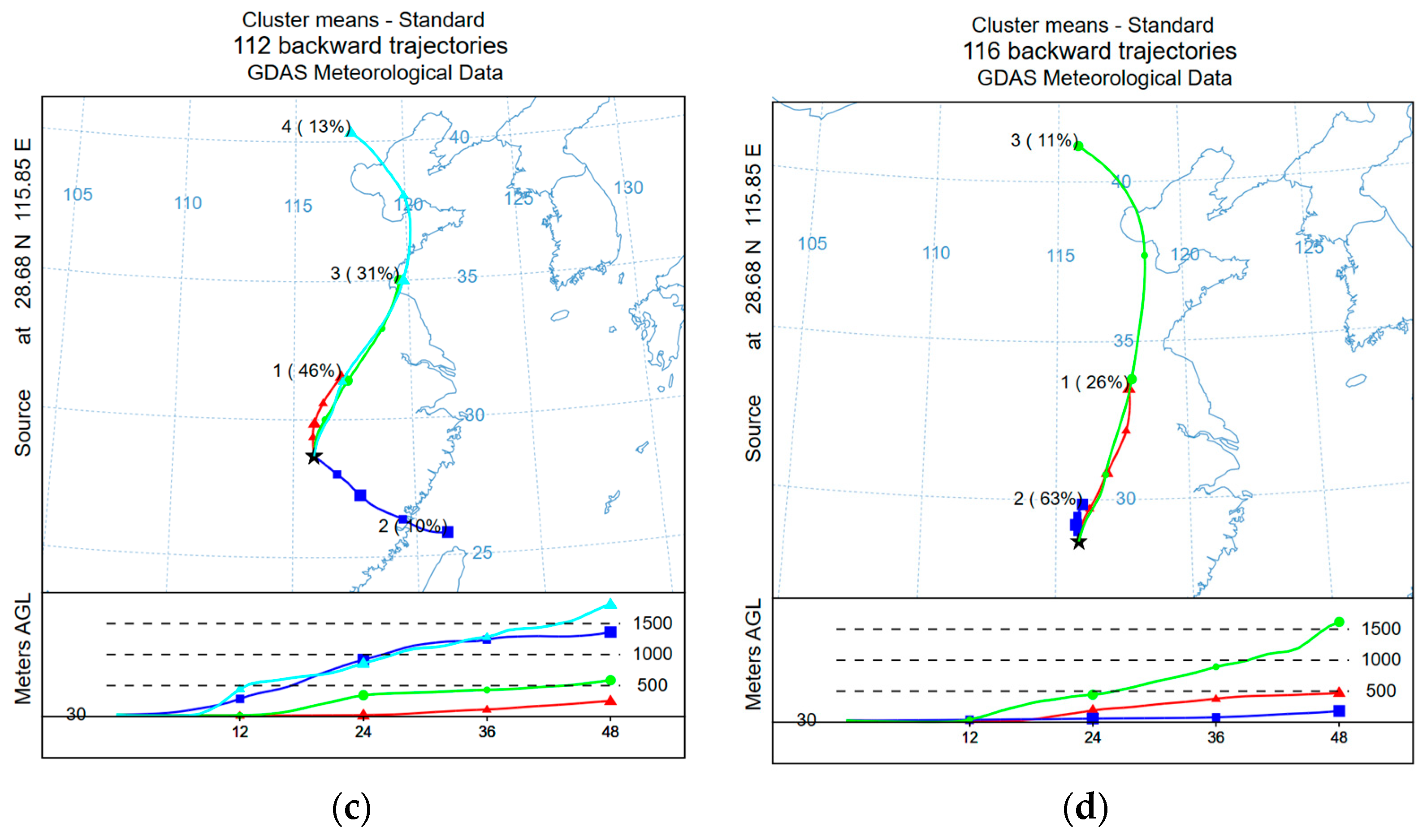
3.2.4. Source Analysis Based on the Backward Trajectory Method
4. Conclusions
Author Contributions
Funding
Institutional Review Board Statement
Informed Consent Statement
Data Availability Statement
Conflicts of Interest
References
- Zhang, Y.L.; Liu, D.; Shen, Z.D.; Ding, B.; Zhang, G.B. Development of a preparation system for the radiocarbon analysis of organic carbon in carbonaceous aerosols in China. Nucl. Instrum. Methods Phys. Res. Sect. B Beam Interact. Mater. At. 2010, 268, 2831–2834. [Google Scholar] [CrossRef]
- Wan, Z.C.; Song, K.; Zhu, W.F.; Yu, Y.; Wang, H.; Shen, R.Z.; Tan, R.; Lv, D.Q.; Gong, Y.Z.; Yu, X.N.; et al. A Closure Study of Secondary Organic Aerosol Estimation at an Urban Site of Yangtze River Delta, China. Atmosphere 2022, 13, 1679. [Google Scholar] [CrossRef]
- Li, X.R.; Wang, Y.F.; Guo, X.Q.; Wang, Y.S. Size Distribution and Characteristics of EC and OC in Aerosols During the Olympics of Beijing, China. Environ. Sci. 2011, 32, 313–318. [Google Scholar]
- Niu, Z.C.; Zhang, F.W.; Kong, X.R.; Chen, J.S.; Yin, L.Q.; Xu, L.L. One-year measurement of organic and elemental carbon in size-segregated atmospheric aerosol at a coastal and suburban site in Southeast China. J. Environ. Monit. JEM 2012, 14, 2961–2967. [Google Scholar] [CrossRef] [PubMed]
- Shangping, J.; Litao, W.; Le, Z.; Qi, M.Y.; Lu, X.H.; Wang, Y.; Liu, Z.T.; Tan, J.Y.; Liu, Y.Y.; Du, C. Concentrations, sources and changes of carbon fractions in PM2.5 in Handan. J. Environ. Sci. 2019, 39, 2873–2880. [Google Scholar]
- Srinivas, B.; Sarin, M.M. PM2.5, EC and OC in atmospheric outflow from the Indo-Gangetic Plain: Temporal variability and aerosol organic carbon-to-organic mass conversion factor. Sci. Total Environ. 2014, 487, 196–205. [Google Scholar] [CrossRef]
- He, K.B.; Yang, F.M.; Ma, Y.L.; Zhang, Q.; Yao, X.H.; Chan, C.K.; Cadle, S.; Chan, T.; Mulawa, P. The characteristics of PM2.5 in Beijing, China. Atmos. Environ. 2001, 35, 4959–4970. [Google Scholar] [CrossRef]
- Juda-Rezler, K.; Reizer, M.; Maciejewska, K.; Blaszczak, B.; Klejnowski, K. Characterization of atmospheric PM2.5 sources at a Central European urban background site. Sci. Total Environ. 2020, 713, 136729. [Google Scholar] [CrossRef] [PubMed]
- Liu, S.; Ma, T.; Yang, Y.; Gao, J.; Peng, L. Chemical Composition Characteristic and Source Apportionment of PM2.5 during Winter in Taiyuan. Environ. Sci. 2019, 40, 1537–1544. [Google Scholar]
- Zou, C.W.; Wang, J.Y.; Hu, K.Y.; Li, J.L.; Yu, C.L.; Zhu, F.X.; Huang, H. Distribution Characteristics and Source Apportionment of Winter Carbonaceous Aerosols in a Rural Area in Shandong, China. Atmosphere 2022, 13, 1858. [Google Scholar] [CrossRef]
- Shen, S.; Liu, L.; Wen, W.; Xing, Y.; Su, W.; Sun, J.Q. Pollution characterization and source analysis of carbon components of PM2.5 in Beijing and surrounding areas in summer. Environ. Eng. 2022, 40, 71–80. [Google Scholar]
- Zhang, L.B.; Sun, P.; Luo, S.N. Characteristics and Sources Analysis of Organic Carbon and Elemental Carbon Pollutionin in PM10 in Harbin City. Environ. Sci. Manag. 2020, 45, 130–133. [Google Scholar]
- Li, Z.; Li, J.; Wang, S.; Zheng, X.B.; Qu, J. Characteristics and Sources Analysis of Organic Carbon and Elemental Carbon in PM10 in Shenyang City. Environ. Sci. Manag. 2020, 45, 113–117. [Google Scholar]
- Pei, Y.X.; Wang, H.L.; Tan, Y.; Zhu, B.; Zhao, T.L.; Lu, W.; Shi, S.S. Analysis of BC Pollution Characteristics under PM2.5 and O3 Pollution Conditions in Nanjing from 2015 to 2020. Atmosphere 2022, 13, 1440. [Google Scholar] [CrossRef]
- Huang, H.; Zou, C.W.; Cao, J.J.; PoKeung, T. Carbonaceous Aerosol Characteristics in Outdoor and Indoor Environments of Nanchang, China, during Summer. Air Waste Manag. Assoc. 2009, 61, 1262–1272. [Google Scholar] [CrossRef] [PubMed]
- Zou, C.W.; Zhang, Y.K.; Gao, Y.T.; Mao, X.Y.; Huang, H.; Tan, Y.L. Characteristics, distribution, and sources of particulate carbon in rainfall collected by a sequential sampler in Nanchang, China. Atmos. Environ. 2020, 235, 117619. [Google Scholar] [CrossRef]
- Huang, H.; Zou, C.W.; Cao, J.J.; PoKeung, T.; Zhu, F.X.; Yu, C.L.; Xue, S.J. Water-soluble Ions in PM2.5 on the Qianhu Campus of Nanchang University, Nanchang City: Indoor-Outdoor Distribution and Source Implications. Aerosol Air Qual. Res. 2012, 12, 435–443. [Google Scholar] [CrossRef] [Green Version]
- Chang, Q. Study on the Distribution Characteristics of Organic and Elemental Carbon in Atmospheric Particles in Shijiazhuang City. Master’s Thesis, Hebei University of Science and Technology, Shijiazhuang, China, 2015. [Google Scholar] [CrossRef]
- Shen, Y.; Liu, J.G.; Lu, V.; Ding, Q.; Shi, J.G. Comparative of Thermal-Optical Transmission and Thermal-Optical Reflectance Methods of Measurement of Organic and Elemental Carbon in Atmospheric Aerosol. J. Atmos. Environ. Opt. 2011, 6, 450–456. [Google Scholar]
- Wang, Y.J.; Dong, Y.P.; Feng, J.L.; Guan, J.J.; Zhao, W.; Li, H.J. Characteristics and influencing factors of carbon-containing substances in PM2.5 in Shanghai. Environ. Sci. 2010, 31, 1755–1761. [Google Scholar]
- Li, R.; Wang, J.; Xue, K.X.; Fang, C.S. Spatial and temporal distribution characteristics and influencing factors analysis of particulate matter pollution in Jinan City. Air Qual. Atmos. Health 2021, 14, 1267–1278. [Google Scholar] [CrossRef]
- He, Q.; Guo, Q.H.; Umeki, K.; Ding, L.; Wang, F.C.; Yu, G.S. Soot formation during biomass gasification: A critical review. Renew. Sustain. Energy Rev. 2021, 139, 110710. [Google Scholar] [CrossRef]
- Xue, F.L.; Niu, H.Y.; Wu, Z.X.; Ren, X.L.; Li, S.J.; Wang, J.X.; Yue, L.; Fan, J.S. Pollution characteristics of organic and elemental carbon in PM2.5 and PM10 in Handan City. Environ. Chem. 2021, 40, 3246–3257. [Google Scholar]
- Dong, G.M.; Tang, G.Q.; Zhang, J.K.; Liu, Q.; Yan, G.X.; Cheng, M.T.; Wenkang, G.; Yinghong, W. Characterization of carbonaceous fraction in PM2.5 in southern Beijing city. Environ. Sci. 2020, 41, 4374–4381. [Google Scholar]
- Liu, J.J.; Hu, X.Z.; Huang, F.L.; Luo, Y.; Ma, S.X. Pollution characteristics of organic and elemental carbon in PM2.5 in Guangzhou. J. Hunan Univ. Sci. Technol. (Nat. Sci. Ed.) 2019, 34, 111–117. [Google Scholar]
- Li, Z.; Li, J.; Wang, S.; Han, Y.Y.; Qu, J. Characteristics and source analysis of organic and elemental carbon pollution in PM2.5 in Shenyang city in spring and summer. Environ. Sci. Manag. 2019, 44, 100–105. [Google Scholar]
- Zhao, M.F.; Qiao, T.; Huang, Z.S.; Zhu, M.Y.; Xu, W.; Xiu, G.L.; Tao, J.; Li, S.C. Comparison of ionic and carbonaceous compositions of PM2.5 in 2009 and 2012 in Shanghai, China. Sci. Total Environ. 2015, 536, 695–703. [Google Scholar] [CrossRef]
- Li, H.M.; Wang, Q.G.; Yang, M.; Li, F.Y.; Wang, J.H.; Sun, Y.X.; Wang, C.; Wu, H.F.; Qian, X. Chemical characterization and source apportionment of PM2.5 aerosols in a megacity of Southeast China. Atmos. Res. 2016, 181, 288–299. [Google Scholar] [CrossRef]
- Soleimanian, E.; Mousavi, A.; Taghvaee, S.; Sowlat, M.H.; Hasheminassab, S.; Polidori, A.; Sioutas, C. Spatial trends and sources of PM2.5 organic carbon volatility fractions (OCx) across the Los Angeles Basin. Atmos. Environ. 2019, 209, 201–211. [Google Scholar] [CrossRef]
- Maritz, P.; Beukes, J.P.; van Zyl, P.G.; Liousse, C.; Gardrat, E.; Ramandh, A.; Mkhatshwa, G.V. Temporal and source assessments of organic and elemental carbon at sites in the northern South African interior. J. Atmos. Chem. 2019, 76, 263–287. [Google Scholar] [CrossRef]
- Jeong, C.H.; Traub, A.; Huang, A.; Hilker, N.; Wang, J.M.; Herod, D.; Dabek-Zlotorzynska, E.; Celo, V.; Evans, G.J. Long-term analysis of PM2.5 from 2004 to 2017 in Toronto: Composition, sources, and oxidative potential. Environ. Pollut. 2020, 263, 114652. [Google Scholar] [CrossRef]
- Kim, K.H.; Sekiguchi, K.; Furuuchi, M.; Sakamoto, K. Seasonal variation of carbonaceous and ionic components in ultrafine and fine particles in an urban area of Japan. Atmos. Environ. 2011, 45, 1581–1590. [Google Scholar] [CrossRef]
- Yu, G.H.; Park, S. Chemical characterization and source apportionment of PM2.5 at an urban site in Gwangju, Korea. Atmos. Pollut. Res. 2021, 12, 101092. [Google Scholar] [CrossRef]
- Sandeep, K.; Negi, R.S.; Panicker, A.S.; Gautam, A.S.; Bhist, D.S.; Beig, G.; Murthy, B.S.; Latha, R.; Singh, S.; Das, S. Characteristics and Variability of Carbonaceous Aerosols over a Semi Urban Location in Garhwal Himalayas. Asia-Pac. J. Atmos. Sci. 2019, 56, 455–465. [Google Scholar] [CrossRef]
- Chow, J.C.; Watson, J.G.; Zhiqiang, L.; Lowenthal, D.H.; Frazier, C.A.; Solomon, P.A.; Thuillier, R.H.; Magliano, K. Descriptive analysis of PM2.5 and PM10 at regionally representative locations during SJVAQS/AUSPEX. Atmos. Environ. 1996, 30, 2079–2112. [Google Scholar] [CrossRef]
- Cao, J.J.; Wu, F.; Zhou, J.C.; Li, S.C.; Li, Y.H.; Chen, S.H.; An, Z.S.; Feng, G.Q.; Watson, J.G.; Zhu, C.S.; et al. Characterization and source apportionment of atmospheric organic and elemental carbon during fall and winter of 2003 in Xi’an, China. Atmos. Chem. Phys. 2005, 5, 3127–3137. [Google Scholar] [CrossRef] [Green Version]
- Zhang, W.J.; Li, M.; Fu, H.X.; Ge, X.; Lv, B.; Wang, Z.F.; Li, H.B. Analysis of PM2.5 chemical components and pollution characteristics in Jinan. Environ. Pollut. Prev. 2019, 41, 1490–1494. [Google Scholar]
- Turpin, B.J.; Huntzicker, J.J. Identification of secondary organic aerosol episodes and quantitation of primary and secondary organic aerosol concentrations during SCAQS. Atmos. Environ. 1995, 29, 3527–3544. [Google Scholar] [CrossRef]
- Pio, C.; Cerqueira, M.; Roy, M.; Harrison, R.M.; Nunes, T.; Mirante, F.; Alves, C.; Oliveira, C.; Campa, A.S.; Artíñano, B.; et al. OC/EC ratio observations in Europe: Re-thinking the approach for apportionment between primary and secondary organic carbon. Atmos. Environ. 2020, 235, 117619. [Google Scholar] [CrossRef]
- Chen, Y.J.; Zhi, G.R.; Feng, Y.L.; Fu, J.M.; Feng, J.L.; Sheng, G.Y. Measurements of emission factors for primary carbonaceous particles from residential raw-coal combustion in China. Geophys. Res. Lett. 2006, 33. [Google Scholar] [CrossRef]
- Han, Y.M.; Cao, J.J.; Li, S.C.; He, G.F.; An, Z.S. Different characteristics of char and soot in the atmosphere and their ratio as an indicator for source identification in Xi’an, China. Atmos. Chem. Phys. 2010, 10, 595–607. [Google Scholar] [CrossRef] [Green Version]
- Chow, J.C.; Watson, J.G.; Kuhns, H.; Etyemezian, V.; Lowenthal, D.H.; Crow, D.; Kohl, S.D.; Engelbrecht, J.P.; Green, M.C. Source profiles for industrial, mobile, and area sources in the Big Bend Regional Aerosol Visibility and Observational study. Chemosphere 2004, 54, 185–208. [Google Scholar] [CrossRef] [PubMed]
- Feng, J.L.; Yu, H.; Su, X.F.; Liu, S.H.; Li, Y.; Pan, Y.P.; Sun, J.H. Chemical composition and source apportionment of PM2.5 during Chinese Spring Festival at Xinxiang, a heavily polluted city in North China: Fireworks and health risks. Atmos. Res. 2016, 182, 176–188. [Google Scholar] [CrossRef]
- Li, X.H.; Wang, S.X.; Duan, L.; Hao, J.M.; Li, C.; Chen, Y.S.; Yang, L. Particulate and trace gas emissions from open burning of wheat straw and corn stover in China. Environ. Sci. Technol. 2007, 41, 6052–6058. [Google Scholar] [CrossRef] [PubMed]
- Jia, X.H.; Xie, J.F.; Ma, X.; Di, Z.D.; Wu, Y.N. Analysis of water-soluble constituents in winter of PM2.5 in Taiyuan city. China Environ. Sci. 2013, 33, 599–604. [Google Scholar]


| Sampling Site | Sampling Time | OC (μg·m−3) | EC (μg·m−3) | References |
|---|---|---|---|---|
| Nanchang | 2021.3–2021.12 | 12.6 | 1.6 | This study |
| Yangquan | 2018.7–2019.3 | 8.0 | 3.6 | [23] |
| Beijing | 2017.12–2018.12 | 11.2 | 1.2 | [24] |
| Guangzhou | 2015.6–2016.05 | 8.2 | 1.8 | [25] |
| Shenyang | 2017.5–2017.8 | 9.6 | 2.3 | [26] |
| Shanghai | 2011.11–2012.12 | 10.7 | 2.0 | [27] |
| Nanjing | 2013.12–2014.10 | 18.0 | 6.7 | [28] |
| Los Angeles, USA | 2012.7–2013.6 | 4.5 | 1.4 | [29] |
| Vanderbilt Park, South Africa | 2009.3–2015.12 | 9.3 | 3.2 | [30] |
| Toronto, Canada | 2014.6–2017.4 | 1.2 | 0.7 | [31] |
| Saitama Prefecture, Japan | 2009.8–2010.4 | 5.5 | 3.3 | [32] |
| Gwangju, Korea | 2013.11–2014.11 | 4.1 | 1.5 | [33] |
| Srinagar, India | 2017.1–2017.12 | 15.3 | 5.2 | [34] |
| Projects | Na+ | NH4+ | K+ | Mg2+ | Ca2+ | Cl− | NO2− | NO3− | SO42− |
|---|---|---|---|---|---|---|---|---|---|
| Annual average | 6.07 | 3.41 | 6.28 | 0.24 | 2.10 | 3.17 | 2.78 | 11.88 | 9.47 |
| Spring | 3.95 | 4.33 | 7.75 | 0.37 | 2.42 | 5.58 | 2.12 | 2.12 | 2.12 |
| Summer | 3.58 | 1.20 | 2.26 | 0.14 | 1.61 | 1.95 | 2.11 | 8.07 | 7.71 |
| Autumn | 8.29 | 3.37 | 6.47 | 0.19 | 2.09 | 2.34 | 3.25 | 14.17 | 10.59 |
| Winter | 14.04 | 7.40 | 8.64 | - | 2.67 | 7.20 | 4.20 | 25.62 | 13.64 |
Disclaimer/Publisher’s Note: The statements, opinions and data contained in all publications are solely those of the individual author(s) and contributor(s) and not of MDPI and/or the editor(s). MDPI and/or the editor(s) disclaim responsibility for any injury to people or property resulting from any ideas, methods, instructions or products referred to in the content. |
© 2023 by the authors. Licensee MDPI, Basel, Switzerland. This article is an open access article distributed under the terms and conditions of the Creative Commons Attribution (CC BY) license (https://creativecommons.org/licenses/by/4.0/).
Share and Cite
Huang, H.; Yin, X.; Tang, Y.; Zou, C.; Li, J.; Yu, C.; Zhu, F. Seasonal Distribution and Source Apportionment of Chemical Compositions in PM2.5 in Nanchang, Inland Area of East China. Atmosphere 2023, 14, 1172. https://doi.org/10.3390/atmos14071172
Huang H, Yin X, Tang Y, Zou C, Li J, Yu C, Zhu F. Seasonal Distribution and Source Apportionment of Chemical Compositions in PM2.5 in Nanchang, Inland Area of East China. Atmosphere. 2023; 14(7):1172. https://doi.org/10.3390/atmos14071172
Chicago/Turabian StyleHuang, Hong, Xin Yin, Yuan Tang, Changwei Zou, Jianlong Li, Chenglong Yu, and Fangxu Zhu. 2023. "Seasonal Distribution and Source Apportionment of Chemical Compositions in PM2.5 in Nanchang, Inland Area of East China" Atmosphere 14, no. 7: 1172. https://doi.org/10.3390/atmos14071172