Impact of Solvent Emissions on Reactive Aromatics and Ozone in the Great Lakes Region

Abstract

While transportation emissions have declined over the past several decades, volatile organic compound (VOC) emissions from solvent use applications have increased as urban areas expand. In this work, the Canadian air quality model (GEM-MACH-TEB) is used to assess the importance of solvent emissions during the Michigan Ontario Ozone Source Experiment (MOOSE). Model predictions are compared to ozone and total mono-substituted aromatics (TOLU) observations collected in Windsor, Ontario. For summer 2018, model estimates of TOLU from solvent emissions are smaller (30% for an 8 h daytime average) in Windsor than estimates from positive matrix factorization (44% for a 24 h average). The use of updated U.S. solvent emissions from the EPA’s VCPy (Volatile Chemical Product framework) for summer 2021 simulations increases the solvent use source contribution over Detroit/Windsor (30–50% for an 8 h daytime average). This also provides a more uniform spatial distribution across the U.S./Canada border (30–50% for an 8 h daytime average). Long-chain alkanes are the dominant speciation in the model’s air pollutant emission inventory and in the observation-derived solvent use factor. Summertime 8 h daytime ozone decreased by 0.4% over Windsor for a 10% solvent use VOC emission reduction scenario. A 10% mobile NO_x emission reduction scenario resulted in a 0.6% O₃ decrease over Windsor and more widespread changes over the study region.

1. Introduction

The emission of volatile organic compounds (VOCs) into the atmosphere leads to the formation of ozone (O₃) and secondary organic aerosol, which are air contaminants associated with adverse health effects [1]. Air pollution is the fifth-largest human health risk globally [2]. Decades of emission regulation in North America and Europe have decreased the number of O₃ exceedance periods annually; however, urban, suburban, and industrial areas still observe a persistent number of non-attainment days of national air quality standards [3]. Currently, the Canadian Ambient Air Quality Standard for O₃ is 62 ppbv for an 8 h daily average and it will decrease to 60 ppbv in 2025.

There have been several air quality modelling studies in the Great Lakes region [4,5,6,7] focusing on the chemical and meteorological processes responsible for O₃ episodes. Makar et al., 2010 used the AURAMS model to simulate O₃ along lake breeze fronts during the BAQS-Met study and found toluene to be an important O₃ precursor downwind of Windsor/Detroit [8]. McNider et al., 2018 used the WRF and CMAQ models and showed improved O₃ forecasts over Lake Michigan when using a land surface scheme driven by data assimilation [9]. Stroud et al., 2020 used the Environment and Climate Change Canada’s (ECCC) GEM-MACH-TEB (Global Environmental Multiscale Model for Air Quality and Chemistry—Town Energy Balance) model to study the O₃ production chemical regime along lake breeze fronts during the 2015 Pan American Games [10]. They found that in suburban Toronto, the most efficient O₃ production occurred in the updraft region of the lake-breeze front, as the precursors underwent vertical mixing. In the updraft region, the O₃ production switched from VOC-sensitive to NO_x-sensitive, and the local net O₃ production rate reached a maximum.

VOCs have both anthropogenic and biogenic sources. As VOC emissions from combustion sources have declined over the past few decades, several studies have shown that emissions from volatile solvent use have become more important sources of VOCs in urban areas [11,12,13,14,15]. Sources considered here for volatile solvent use include personal care products, fragrances, pesticides, coatings, adhesives, and printer inks. A recent American study estimated that, at national and urban scales, 15 to 42% of petrochemical VOCs are attributed to mobile sources and 39 to 62% to solvent use, with the remainder attributed to the oil and gas sector [15]. Coggon et al., 2021 modelled an O₃ exceedance event in New York City and found that volatile solvent emissions contributed an additional 10 ppbv of O₃ [16]. Certain volatile solvents are also of direct concern to environmental health because they are known toxins (e.g., benzene and toluene) [17].

A complete understanding of the impact of solvent emissions on air quality is based on our knowledge of solvent emission inventories. However, emission inventories are not well constrained due to uncertainties in formulation, usage patterns, volatility, building exchange, and product fate [18]. Air quality models rely on bottom-up estimates from emission inventories. However, few studies have evaluated the representativeness of these emission estimates by comparing them with ambient measurements. Indeed, recent studies have shown that regulatory inventories may underestimate solvent emissions by a factor of 2–3 [15]. The validation of existing emission inventories and an evaluation of their use in air quality models are needed [19,20].

The major goal of this study is to use the GEM-MACH air quality model to assess the contribution of solvents to several important VOC species (e.g., toluene and ethylbenzene) that are measured in Canadian urban areas. This study is novel in that it compared top-down and bottom-up methods for source apportionment, as shown in Figure 1. The results for MOOSE 2021 will use a US emission inventory with solvent emissions calculated using the VCPy emission model [20]. The second goal of this study is to calculate the sensitivity of the model-predicted O₃ to two emission scenarios: (1) a 10% reduction in solvent emissions and (2) a 10% reduction in mobile NOx emissions. The scenarios are designed to help inform the mitigation of ozone air pollution in the Great Lakes region.

2. Materials and Methods

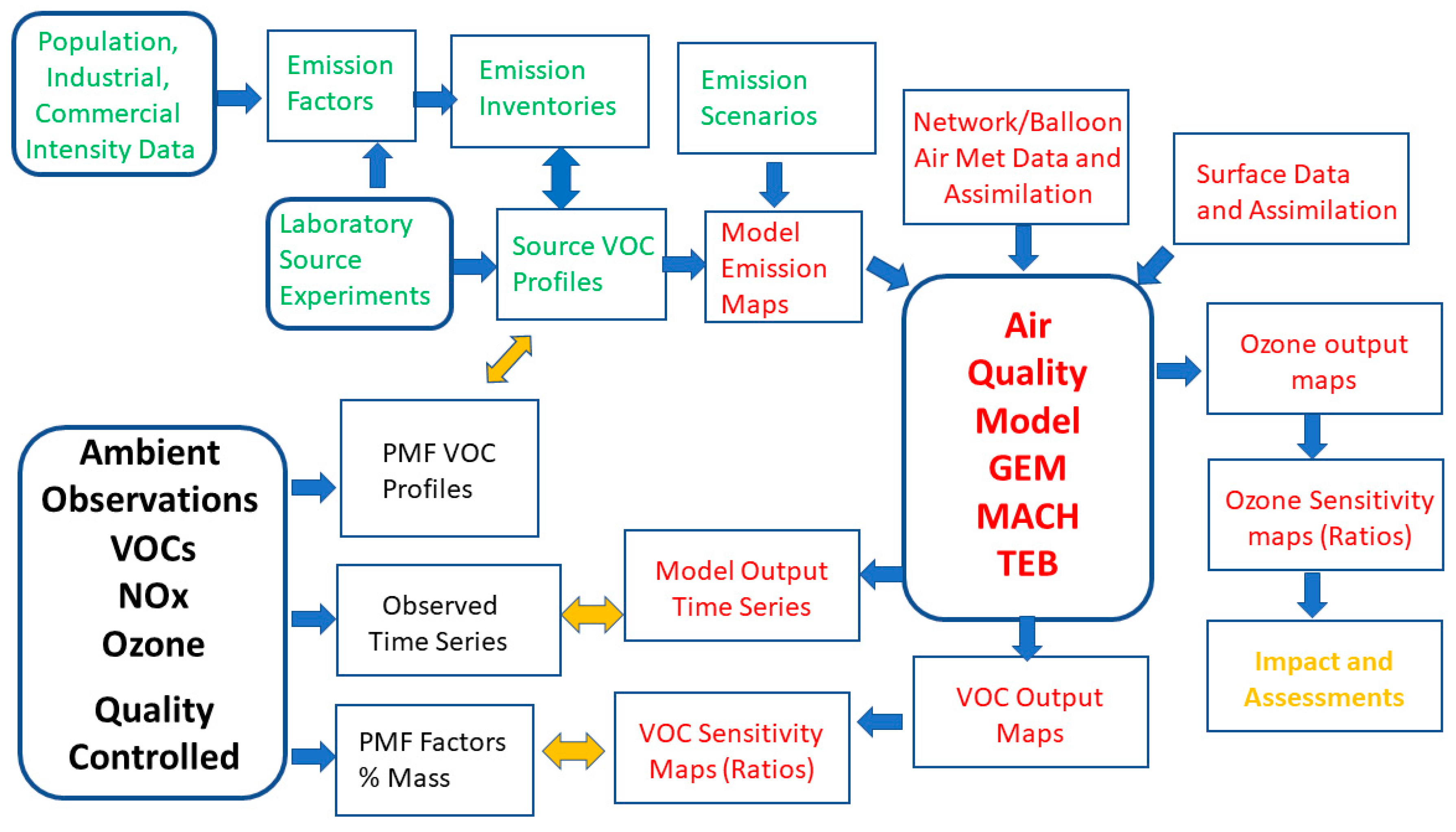
2.1. GEM-MACH-TEB Model Description and Setup

Air quality simulations were performed using Environment and Climate Change Canada’s operational air quality forecast model, GEM-MACH. The 3D atmospheric model is online with routines describing air quality processes (e.g., pollutant vertical eddy diffusion, atmospheric chemistry, and pollutant deposition) called from the physics operator in the GEM weather forecast model [21]. The model version (GEM v4.9, GEM-MACH v2.9) and configuration are described in detail by Stroud et al., 2020 [10]. In brief, the operational GEM-MACH model (North American continental domain with 10 km grid cell spacing) was used to provide the chemical lateral boundary conditions for a higher-resolution simulation (Great Lakes domain with 2.5 km grid cell spacing). The model surface scheme is based on the advanced soil moisture and land surface temperature assimilation system, termed CALDAS (Canadian Land Data Assimilation System [22]. The Town Energy Balance (TEB) scheme was used to simulate the urban heat island effect by including terms in the surface heat flux for buildings (roof and walls), roads, and vehicle exhaust [23,24].

Table 1. List of VOC species considered in the GEM-MACH-TEB model.

Chemical Species	Acronym	OH-Rate Coefficient (298 K, cm3/molec/s)
Ethane	C2H6	2.72 × 10−13
Propane + Benzene + Acetylene	C3H8	1.18 × 10−12
Ethene	ETHE	8.54 × 10−12
Isoprene	ISOP	8.03 × 10−11
Long chain alkene	ALKE	3.88 × 10−11
Long chain alkane	ALKA	4.56 × 10−12
Multi-substituted aromatic	AROM	3.94 × 10−11
Mono-substituted aromatic	TOLU	6.19 × 10−12
Cresol species	CRES	4.00 × 10−11
Ketone species	MEK	9.85 × 10−13
Formaldehyde	HCHO	1.11 × 10−11
Aldehyde species	ALD	1.59 × 10−11

Note: Ethane is considered as a constant concentration vertical profile.

lists the VOC chemical speciation used in GEM-MACH-TEB [25]. The gas-phase chemical mechanism includes 47 species and 114 reactions. This mechanism was developed for continental conditions with moderate-to-high NO_x concentrations [26,27]. This mechanism includes radical production from photolysis reactions (e.g., ozone, formaldehyde, hydrogen peroxide, and nitrous oxide). Organic species are generally represented by shorter-lived and longer-lived species for each functional group class (e.g., formaldehyde and a combined higher carbon number aldehyde species). The reactions of O₃, OH, and NO₃ are considered for organic species oxidation. The mapping of explicitly emitted species to combined mechanism species was mole-based with a weighting applied to conserve the OH reactivity. The major nitrogen species in GEM-MACH include NO, NO₂, NO₃, HONO, HNO₃, HNO₄, N₂O₅, RNO_3, and PANs.

The model was run on a Cray XC40 supercomputer. For this study, 24 h forecasts over a two-month period (June–July 2018) were used, with the atmospheric fields updated based on an assimilated meteorology analysis. Three-dimensional chemistry fields were recycled (i.e., a chemistry field from the end of the 24 h cycle is used to initialize the next cycle). Simulations for the MOOSE (summer 2021) were also performed using the updated GEM meteorology model (v5.0) and updated emissions described in the next section.

2.2. Pollutant Emission Inventories and Emission Processing

For the 2018 model simulations, the 2015 Canadian Air Pollutant Emission Inventory (APEI, https://www.canada.ca/en/environment-climate-change/services/pollutants/air-emissions-inventory-overview.html URL (accessed on 28 January 2022)) was used, including emissions reported in the 2015 Canadian National Pollutant Release Inventory (NPRI, https://www.canada.ca/en/services/environment/pollution-waste-management/national-pollutant-release-inventory.html URL (accessed on 28 January 2022)) for relatively large facilities that meet the reporting threshold [28]. For the US, the projected 2017 emissions from the 2011 Version 6.3 Platform (https://www.epa.gov/air-emissions-modeling/2011-version-63-platform URL (accessed on 28 January 2022)) with updated 2018 point source emissions were used. For US on-road mobile emissions, the MOVES2014a traffic model was used with 2017 real activity data, which helped to correct the known Nox on-road emission over-predictions in the 2011 National Emissions Inventory (NEI). The U.S. EPA SPECIATE database (v4.5) was used for the VOC and PM speciation profiles (https://www.epa.gov/air-emissions-modeling/speciate-2 URL (accessed on 30 January 2022)). Table S1 lists the non-mobile area emission subclass codes (mainly solvent use, surface coatings, and residential wood combustion) for the 2015 Ontario and Source Classification Codes (SCC). Table S2 lists the Ontario 2015 non-mobile area inventories ranked by emission strength. Table S3 lists the Michigan projected inventory for solvent emissions used for the 2018 simulations. Due to differences in the detailed sources of solvent emissions available in each national inventory, 37 speciation profiles were used to process U.S. VOC emissions, while 12 speciation profiles were used to process Canadian VOC emissions. Table S4 lists the TOG speciation profiles for the chemical mechanism used in GEM-MACH. Annual total solvent emissions were allocated equally across months, days of the week, and times of the day. Future work will consider the temperature dependence in solvent emission temporal allocation.

Simulations for MOOSE 2021 were performed with the Canadian 2015-based projected 2020 emissions and U.S. 2017 emissions compiled for the EPA’s Air Quality Time Series (EQUATES; www.epa.gov/cmaq/EQUATES URL (accessed on 01 February 2023)) project [11] with updated 2018 point source emissions. Speciation for US solvent emissions was updated for the 2021 simulations based on EPA’s VCPy methodology, which includes 16 updated TOG speciation profiles [20]. Table S5 lists the 2017 Michigan solvent SCCs ranked by emission strength and includes the TOG speciation profile numbers and descriptions. Table S6 lists the TOG profiles used to process the US VCPy solvent emissions in the GEM-MACH chemical speciation.

The area emissions in the summer are dominated by solvent use. Solvent use includes consumer and commercial product use (personal care products, other household products, commercial pesticide application, aftermarket auto finishing, adhesives, and sealants) and industrial applications (adhesives and general solvents). In the emission inventories, solvent use classification includes surface coatings from construction, primary industry, manufacturing, distribution/retail, transportation modes, and private household use. Dry cleaning, graphic art printing, rubber product use, and degreasing are considered separately but still under general solvent use.

The US and Canadian national emission inventories classify the range of chemicals and subclasses under the term solvent use. For this reason, we have used this terminology throughout; however, it is synonymous with another term, volatile chemical products (VCP), also used in the literature.

2.3. Measurements

A map of the study region is shown in Figure 2. The Windsor West air quality site (latitude 42.292°, longitude −83.073°) is part of the Environment and Climate Change Canada’s National Air Pollution Surveillance (NAPS) network and is co-operated by the Ontario Ministry of Environment Conservation and Parks (OMECP). The Windsor West station is classified as an urban neighborhood site, operated from a schoolyard. NAPS stations continuously measure the mixing ratio of O₃ using hourly data. VOCs are measured at Windsor West every 1 in 6 days using Xon Tech canisters with a 24 h sample time (00:00–24:00 EST), followed by gas chromatography and detection (flame ionization and mass spectrometry) [29]. There were 61 scheduled samples and 107 VOC species reported in 2018. The 107 VOCs consist of alkanes, alkenes, aromatic hydrocarbons, halogenated organics, and other organic compounds, as listed in Table S7.

Among the 61 scheduled samples, 41 samples were reported. Among the 107 VOC species, 72 of them had >60% valid data points. A VOC concentration below its method detection limit was maintained at its detection limit. Missing VOC concentrations were inputted with median values during the study period because the PMF model does not accept missing values. Overall, the data quality of the 24 h integrated VOC concentrations in Windsor for 2018 was good.

2.4. Positive Matrix Factorization (PMF)

The US EPA PMF 5.0 was used to identify the source sectors and to quantify their contributions to ambient VOCs in Windsor in 2018. As a required PMF input, the uncertainty of the measured ambient concentrations was estimated using MDLs and error fraction, with the following formula as suggested by the EPA PMF manual [30].

When the concentration is less than or equal to the MDL,

$$Uncertainty=\frac{5}{6}\times MDL$$

(1)

When the concentration is greater than the MDL,

$$Uncertainty=\sqrt{{\left(Error fraction\times concentration\right)}^2+{\left(0.5\times MDL\right)}^2}$$

(2)

where error fractions for VOCs are equal to 10%, as suggested by other researchers [31].

The PMF was run eleven times with the number of factors increased from 4 to 14, with an increment of 1. The optimal nine-factor solution was retained based on the indicative model performance metrics and the physical interpretability of the factors. A factor profile matrix, one of the model outputs, was used to interpret the source factors. The factor profiles from the PMF model were compared with factor profiles from the literature and emission inventories, and each factor was assigned a factor name. The predicted concentrations of each VOC species were the summation of the product of their values in all factor profiles, with the corresponding factor contributions. The predicted and observed concentrations of VOCs were compared to evaluate the performance of PMF. PMF model performance diagnostics, i.e., observation–prediction time series, the coefficient of determination (R²) value, and slopes were used to evaluate model performance.

Uncertainty analysis (i.e., Bootstrap, BS and Displacement, DISP) tests were performed to assess the uncertainties associated with factor profiles and factor contributions from the nine-factor solution. The result of the BS analysis showed that, on average, 88% (ranging from 80% to 99%) of the resolved factor profiles were re-mapped. These values are acceptable because they met the US EPA’s criterion of BS mapping of 80% [30], suggesting that the number of factors (9) would be appropriate [30]. Furthermore, the results of the DISP analysis suggested that our PMF factor profiles and factor contributions from the nine-factor solution were considered reliable due to the <1% drop in the Q value (defined as the minimum false discovery rate at which an observed score is deemed significant). The minimization of the Q value is the aim of PMF to derive the optimal factor profiles and factor contributions. The small drop in the Q value (≤1%) in the DISP test indicates that the PMF model indeed identified the most appropriate factor profiles and factor contributions.

3. Results

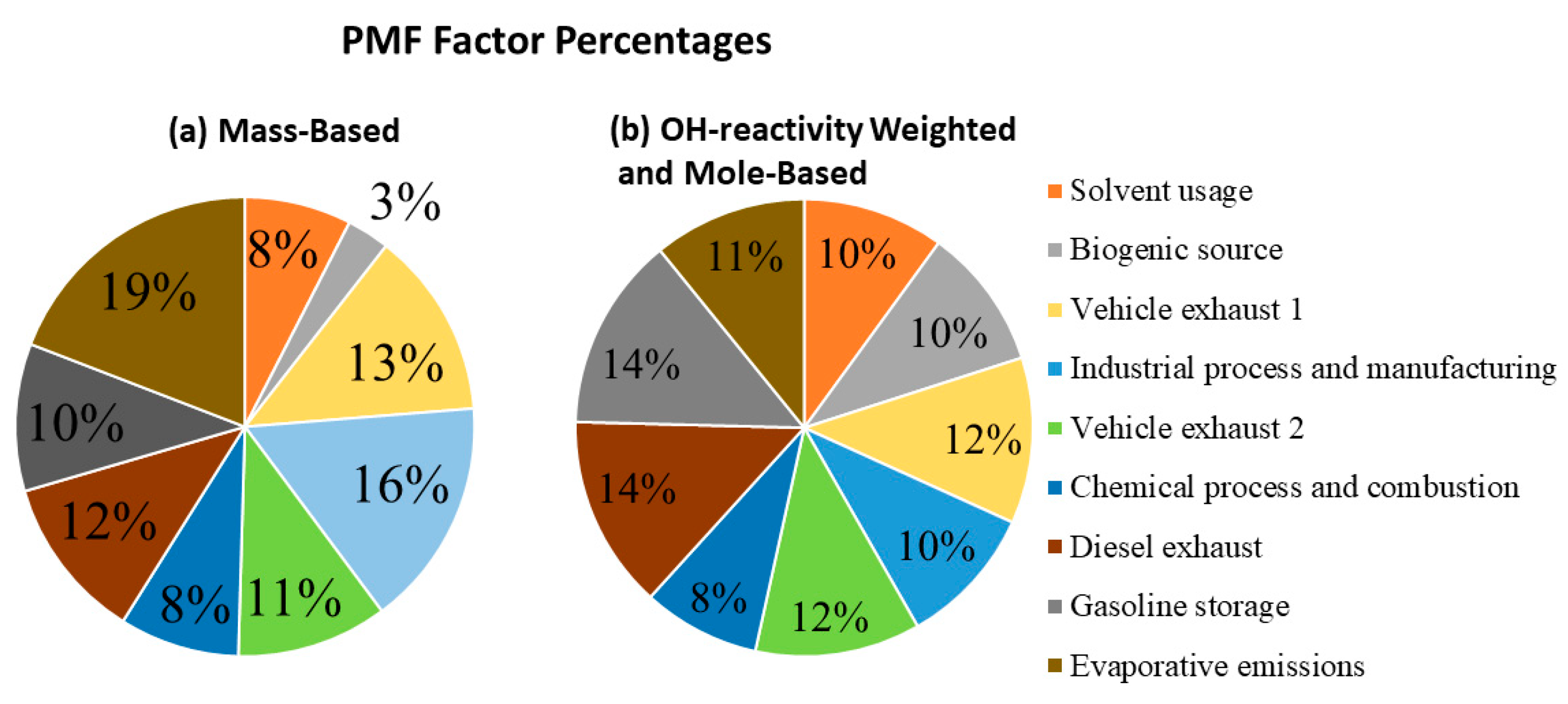
3.1. Positive Matrix Factorization of VOC Data at Windsor West Site

The nine factors resolved by the PMF analysis using VOC data collected at Windsor West in 2018 are as follows: (1) solvent use, (2) biogenic (isoprene), (3) vehicle exhaust 1, (4) vehicle exhaust 2, (5) industrial processes involving halogenated compounds, (6) chemical manufacturing and power generation, (7) diesel exhaust, (8) gasoline production and storage, and (9) natural gas evaporative losses. Solvent usage contributed 8% (by mass) to the total VOC on an annual basis (Figure 3). The three vehicle fuel exhaust factors totalled 36%. The two industrial factors totalled 24%. The two evaporative emission factors totalled 29%.

The solvent usage factor is characterized by high loadings of 1,1-dichloroethylene (64%), toluene (48%), a-pinene (44%), d-limonene (44%), and 1,4-dichlorobenzene (39%), and moderate loadings of m- and p-xylene (33%), o-xylene (31%), and ethylbenzene (30%). Dichloroethylene is used as a solvent for many consumer products (waxes, resins, perfumes, dyes, and lacquers). A-pinene (44%), b-pinene (35%), and d-limonene (44%) are known fragrance compounds. Descriptions of the other eight PMF factors are included in Section S1 (Supplementary Materials) [32,33].

The factor profile of toluene, ethylbenzene, and xylene in the solvent usage factor in this study is similar to the profile of toluene (40%), ethylbenzene (30%), and xylene (40%) in solvent usage factor in an urban Paris study [34]. On average, for summer months, 41% of the total measured mono-aromatics (1.6 μg/m³) were from the PMF solvent usage factor mono-aromatics (0.66 μg/m³). This percentage is compared to the GEM-MACH model results from the sensitivity simulations in Section 3.6.

The source contributions of VOC concentrations in this study are comparable with the findings of a source apportionment study in Windsor using 24 h VOC concentration data collected from 2001 to 2009 [35]. The study quantified the source contributions of VOCs using a chemical mass balance (CMB) model. The study found that vehicle emission was the largest contributor, which accounted for 44% of the total ambient VOC concentrations, followed by industrial sources (19%), commercial natural gas (18%), liquefied petroleum gas (9.3%), coke oven (4.5%), and architectural coating (4.2%), with biogenic emission having the lowest contribution (1%). The decrease in vehicle contribution and increase in solvent use and coatings between the previous data and the current study are consistent with the expected trends in urban population growth and the effectiveness of vehicle exhaust scrubbers.

3.2. Comparison of Solvent Use Factor with Inventory-Weighted Speciation Profiles

For the summertime of 2018 (June–August), the solvent usage factor averaged 2.7 μg/m³ of the total VOC. Toluene and other mono-aromatics in the solvent factor totaled 0.66 μg/m³ in summer, which was 24% of the total solvent VOC. This can be compared to the TOG speciation profiles from various solvent use applications (Table S4), which are used to speciate the emission inventories by subclassifications. Most of the TOG speciation profiles have lower mono-aromatic fractions, except for the solvent used for rubber and plastic product production (Subclass 50402, Profile #1008, TOLU 35%).

Table 2. Weighted TOG (total organic gas) speciation profiles used for processing the solvent emission inventories and the measurement-based factor analysis. For Michigan, P2017 stands for Projected 2017. Similarly, for Ontario, P2020 stands for Projected 2020.

Chemical Species	Weighted Ontario Profile (2015)	Weighted Michigan Profile (P2017)	Weighted Ontario Profile (P2020)	Weighted Michigan Profile (2017)	Weighted Solvent Factor Observed
Isoprene	0	0	0	0	0
Ethane	N/A	N/A	N/A	N/A	0.15
Propane	0.048	0.063	0.067	0.061	0.013
Ethene	0	0	0	0	0.012
Long-chain alkene	0.040	0.0054	0.044	0.0025	0.056
Long-chain alkane	0.53	0.63	0.66	0.66	0.29
Multi-substituted aromatic	0.053	0.068	0.063	0.045	0.14
Mono-substituted aromatic	0.045	0.031	0.054	0.053	0.23
Benzene	0	0	0	0.0017	0
Phenol species	0.0020	0.00085	0.0024	0.0012	0
Ketone species	0.021	0.017	0.027	0.018	0
Aldehyde species	0.000033	0.00011	3.9 × 10−5	0.000024	0
Other	0.25	0.23	0.34	0.30	0.095
Formaldehyde	0	4.2E-6	3.1E-6	0	0

Notes: The modelled allocation is the largest for alkane species, followed by aromatics. The Other category is considerable and was not used in the model system. The solvent factor is also the largest for alkanes but less than the modelled allocation. The solvent factor loads are higher on aromatics than in the model. The alkene species is similar to the Ontario profile values. A significant amount of solvent factor mass loads on ethane. GEM-MACH uses a constant ethane concentration vertical profile, so no emission processing is considered, and the emission allocation is zero.

lists the weighted chemical speciation profiles (by mass) using the solvent use sector in the emission inventories and compares them to the weighted solvent use factor. The inventory solvent using subclass emission (in tons) was used to weigh individual speciation profiles when calculating the annual average profile shown in Table 2. All the annual average profiles are quite similar between the various inventories for each country. The long-chain alkanes and other species have the highest mass fractions. For the oxygenated VOCs, ketones have the largest mass fraction of about 2%. For the weighted solvent factor profile, the long-chain alkenes, long-chain alkanes, multi-substituted aromatics, mono-substituted aromatics, and other species are all important. There are significant differences between the model speciation and factor speciation for long-chain alkenes, long-chain alkanes, and aromatics. The mono-substituted aromatic solvent factor mass fraction is 0.24 compared to the inventory-weighted mass fraction of ~0.05. The alkene PMF value is similar to the Ontario inventory alkene values. A significant amount of solvent factor mass loads on ethane. GEM-MACH uses a constant ethane concentration vertical profile to initialize ethane at each model time step, so no emission processing is considered for ethane in GEM-MACH. The VOC measurements used in the PMF analysis did not include oxygenated VOCs, so a comparison of OVOCs was not possible. Clearly, measurements of OVOCs related to solvent use are needed in the NAPS network or in special field studies. The other category in the model was not used, so the mass was lost from the model system. The other species in the inventory and in the PMF are long-lived species, often halogenated, and do not contribute to O₃ formation at urban-to-regional scales.

3.3. Reactivity Weighting Applied to PMF Solvent Factor

Among the 107 VOC species, the OH-rate coefficients for 101 VOC species at 300 K were obtained from the SAPRC-07 mechanism by Carter, 2010 [36] and other studies [37,38,39,40], as listed in Table S7. The remaining six VOC species, i.e., carbon tetrachloride, Freon 11, Freon 12, Freon 22, Freon 114, and tetrachloroethylene are long-lived; therefore, they were excluded from the OH-reactivity calculations. The concentrations of VOCs were converted to molecule/cm³ and multiplied by their corresponding OH-rate coefficients (cm³ molecule⁻¹ s⁻¹) to obtain the OH-reactivity in units s⁻¹. These OH-reactivities were used to estimate the OH-reactivity-weighted factor contributions by calculating the mole-based OH-reactivities by each PMF resolved factor and the sum of the total OH-reactivities from all factors. The ratios of OH-reactivities for each factor and OH-reactivities from all factors are the weighted percentages shown in Figure 3. The contribution of the solvent use factor increased from 8% (by mass) to 10% (by OH-reactivity). Interestingly, the distribution of factors became even more equally weighted when considering OH-reactivity. This illustrates the diverse nature of emission sources for O₃ formation in the study region.

Among the 107 measured VOC species, the top ten highest OH-reactivity species accounted for 60% of the total OH-reactivity. They are ethylene (12.6%), isoprene (10%), propylene (7.2%), isobutene (6.1%), butane (5.3%), m- and p-xylene (5.1%), propane (4.1%), isopentane (4%), pentane (3%), and toluene (3%). The remaining 97 VOC species contributed to 40% of the total OH-reactivity.

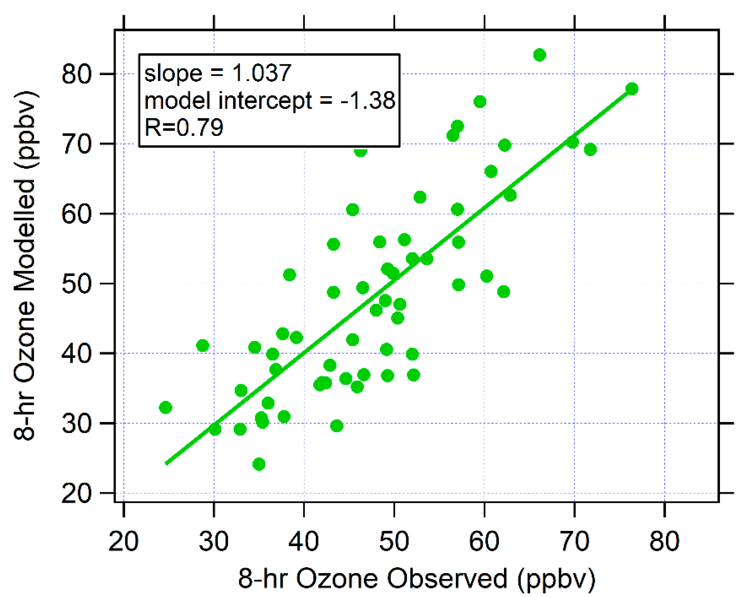
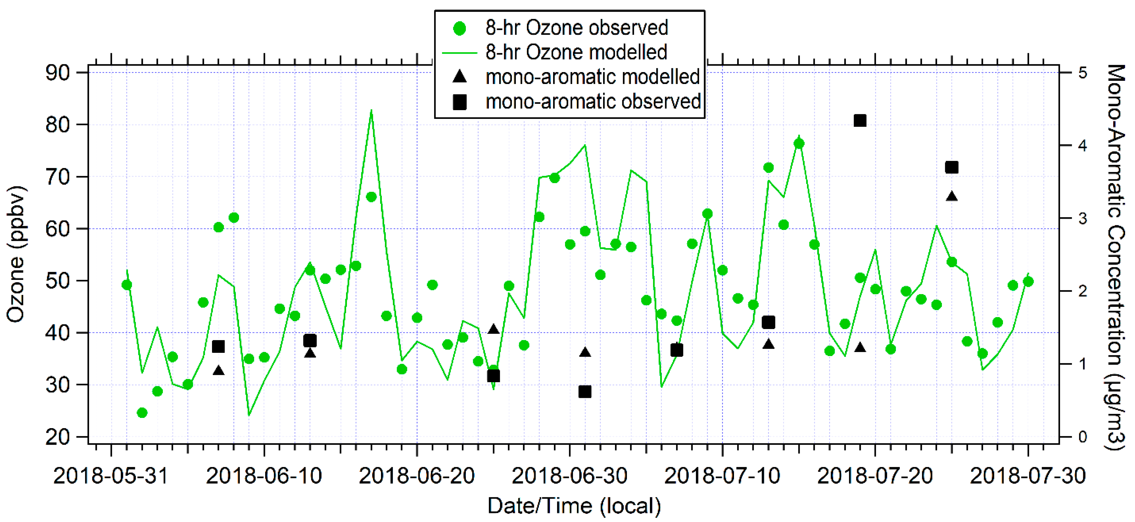
3.4. Validation of O₃ Predictions

The 2.5-km GEM-MACH-TEB air quality model system was recently evaluated for O₃ predictions in the Great Lakes region [10]. The same model system is used in this study but with updated emissions for a more recent meteorological time period. Figure 4 shows the correlation between 8 h daily maximum modelled O₃ and 8 h daily maximum observed O₃ between June and July 2018 at the Windsor West site. The correlation slope is 1.04, the model intercept is −1.4 ppbv, and the correlation coefficient is 0.79. The model performance is similar to the results from prior studies [10] and peer air quality model systems [41,42,43,44,45].

3.5. 2015 Annual Ontario Air Emission Inventories

The combined annual point and area source VOC emissions for the province of Ontario had a total value of 392 ktons, of which the on-road (41 ktons) and off-road (51 ktons) mobile emissions contribute 23% by mass to the total VOC, while the NPRI point sources contribute 13% by mass (49 ktons) and the agricultural emissions contribute 6% by mass (25 ktons). The remaining non-mobile area sources total 226 ktons VOCs (58% by mass). An analysis of the annual 2015 Ontario non-mobile area sources reveals a 56% contribution from solvent use applications. Thus, combining the percentages yields approximately 32% of the total VOC from solvents used in applications on an annual basis.

Table S2 lists the Ontario non-mobile area subclassifications ranked from the highest emission to the lowest emission sources. The top five are as follows: (1) private household use of consumer products, (2) residential wood combustion from wood stoves, (3) solvents used in manufacturing, (4) solvents used in commercial services, and (5) residential wood combustion from fireplaces.

3.6. Air Emission Inventories for a Defined Border Domain

A smaller US/Canada border domain was created to estimate the regional-scale VOC emission budget (Figure S1). The domain centered on Detroit/Windsor and included Port Huron/Sarnia to the north and Cleveland/Toledo to the south. The border domain contained 75% of the land area in the U.S. and 25% in Ontario. If we look at the annual Ontario non-mobile area inventory as a guide, 28% is from cold-season wood combustion and 58% is from solvent use. If we remove the cold-season wood combustion emissions, it is estimated that 82% of the non-mobile area emissions would be from solvent use. For the Ontario region of the border domain, non-mobile areas accounted for 62% of the total area of the Ontario subregion emissions. Therefore, it is estimated that 0.82 × 62% = 51% by mass of the total VOC would be from solvent use in summer on the Canadian side of the border subregion. This percentage of the total VOC is considerably higher than the PMF solvent factor summertime average percentage of 11% by mass. Given the importance of solvent emissions, a 10% emission reduction scenario was performed with GEM-MACH, and the results are shown in Section 3.7.

For the US sub-domain, non-mobile area emissions from P2017 inventories accounted for 53% of the total VOC emissions for the US subregion on an annual basis, which is similar to the Ontario subregion. The top five solvent use SCCs for U.S. emissions (used in 2018 simulations, see Table S3) are as follows: (1) architectural coatings, (2) consumer personal care products, (3) other household products, (4) Federal insecticide-related products, and (5) commercial pesticide applications.

Other important VOC sectors in the border domain are on-road and off-road emissions, totaling 19% on the Canadian side and 38% on the U.S. side. Oil and gas refining and chemical manufacturing accounted for 4.6% on the Canadian side, largely from the Sarnia location. On the Canadian side, agricultural emissions accounted for 9% on an annual basis. Given the importance of mobile emissions, a 10% emission reduction scenario was performed using GEM-MACH, and the results are shown in Section 3.9.

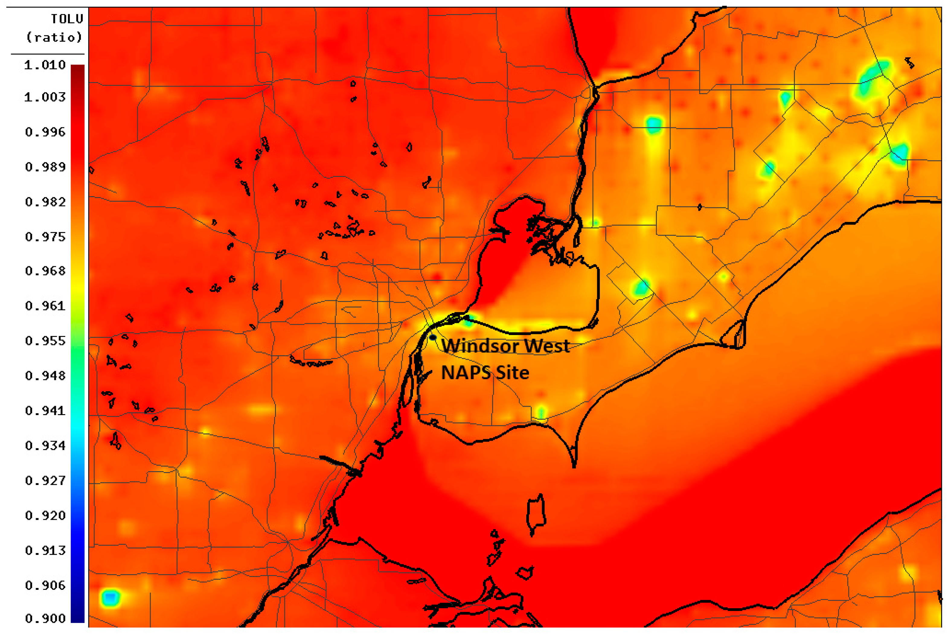
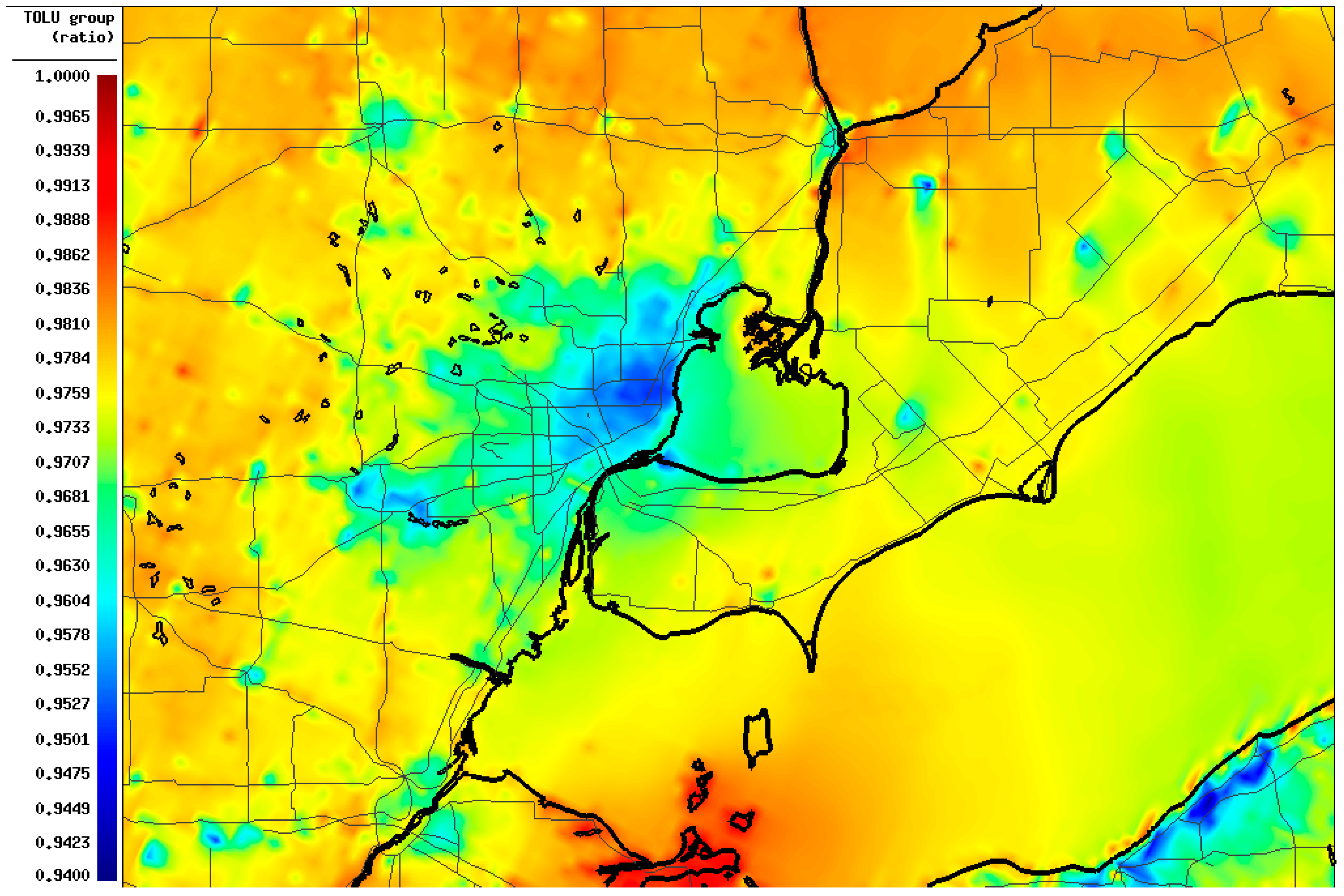
3.7. GEM-MACH Sensitivity Simulation with 10% Solvent Emission Reduction

A sensitivity simulation was performed with a 10% VOC reduction in solvent emissions from applications. This method is referred to as the perturbation approach in the literature [46]. Small perturbations are selected for individual sectors that do not disturb the non-linear O₃ chemical regime in the model. The ratio of the mono-substituted aromatics from the sensitivity and base simulations was calculated and averaged for daytime conditions over the summertime period (e.g., if the mono-aromatic mixing ratios decrease by 1% for a 10% sector emission change, this would represent an approximate 10% solvent use contribution). Figure 5 illustrates the corresponding mono-aromatic sensitivity for summertime and 8 h daytime conditions (averaged for 11 a.m.–7 p.m. local time). The average daytime aromatic ratio at Windsor West is 0.97 (3% decrease), which represents an approximate 30% contribution from the solvent emissions. The blue color in Figure 5 shows ratios of 0.93 (7% decrease) on both sides of the border, which represents an approximate 70% contribution. These are the industrial areas where solvents are applied. An analysis at Windsor West for all hourly model data showed a 3.8%, 1.5%, and 0.7% decrease for the 95th, 50th, and 5th percentiles, respectively, between the emission reduction and base case simulation.

3.8. Case Study Periods

3.8.1. Selecting Year 2018 O₃ Case Study Periods at Windsor West

Figure 6 shows the modelled and measured time series for 8 h daily maximum O₃ and 24 h mono-substituted aromatics (mainly toluene, ethylbenzene, and propyl-benzenes) at Windsor West. High O₃ days at Windsor West are typically under light southwest winds [47]. This wind field was observed on 7 June, 17 June, 29 June, 13 July, and 19 July 2018, and was accompanied by warm temperatures and high O₃ mixing ratios.

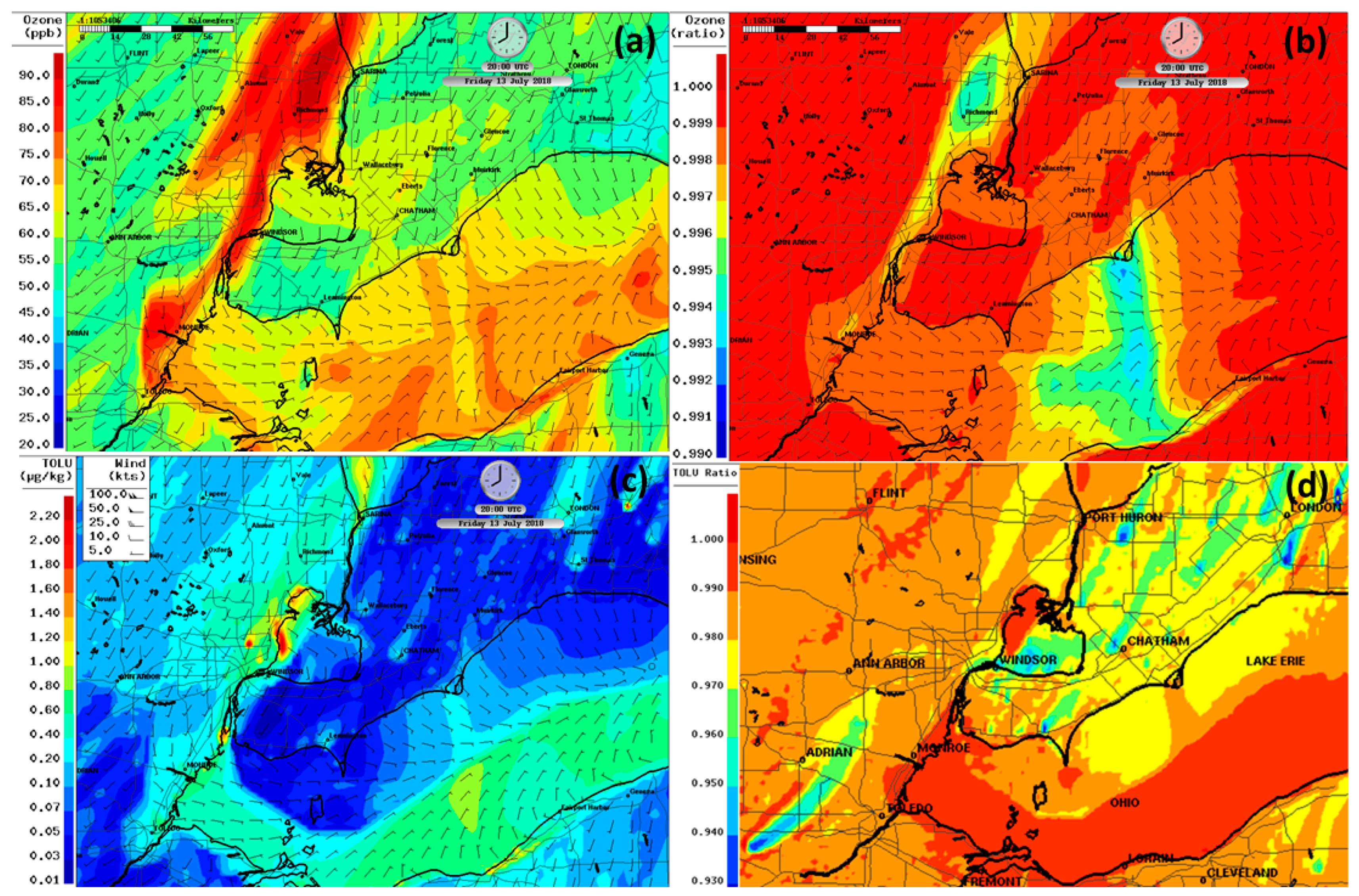
3.8.2. Southwest Wind Pattern

A summary of the model comparison for these days is as follows:

7 June 2018: GEM-MACH-TEB predicted mono-aromatics well but under-predicted the 8 h O₃ maximum by 10 ppbv. The winds were from the south. A complex lake breeze was modelled.

17 June 2018: GEM-MACH-TEB overpredicted the 8 h O₃ maximum by 15 ppbv. Winds were from the southwest, and a complex lake breeze was modelled. There was no VOC collection on this day.

29 June 2018: GEM-MACH-TEB predicted high 8 h O₃ (70 ppbv). A similar mixing ratio was observed (70 ppbv). The winds were light and from the southwest. Lake breeze fronts were predicted by the model in the region. However, no VOC samples were scheduled for collection on this day.

19 July 2018: GEM-MACH-TEB predicted good agreement with the measured O₃ at near-average monthly values. The mono-substituted aromatics were significantly under-predicted. The wind pattern was quite complex on this day, which likely explains the poor model performance of the mono-substituted aromatics.

13 July 2018: GEM-MACH-TEB predicted a high 8 h O₃ (69 ppbv), and a similar mixing ratio was observed (72 ppbv). The mono-substituted aromatics were predicted quite well and at near-average monthly values. The winds were light and from the southwest. Given the availability of data and comparable model predictions, 13 July was selected for further study.

Figure 7a shows the 13 July 2018, 20Z (4 pm local time) modelled O₃ field. A lake breeze formed to the west of Lake Erie. Emissions from Toledo and sources along the western shore of Lake Erie are precursors to the O₃ formed along the lake breeze front. O₃ is photochemically formed from south to north as the air mass travels from Windsor to Detroit and farther north to the western shores of Lake Huron. The O₃ is titrated over western Detroit by local NO emissions. The highest modelled O₃ over Detroit (>85 ppbv) is along a lake breeze front just to the west of Lake St. Clair.

Figure 7b shows the O₃ ratio plot (sensitivity run/base run) for the 10% solvent emission reduction scenario. A ratio of 0.99 represents a 1% O₃ reduction compared to the base case. The lowest ratios (0.992–0.994) are observed downwind of Cleveland over cooler Lake Erie water compared to land, which suppresses vertical mixing. Downwind of Windsor/Detroit, O₃ ratios were from 0.994 to 0.996 on the eastern side of the O₃ plume near Port Huron (0.4–0.6% O₃ decrease and showing VOC-sensitive O₃ production). Interestingly, the western side of the modelled downwind O₃ plume did not show any sensitivity to VOC reduction, indicating that the O₃ production was NO_x-sensitive. The western side also had higher modelled isoprene and formaldehyde, providing VOC reactivity. The lowest ratios in Detroit (from 0.996 to 0.998) are also along the lake breeze front to the west of Lake St. Clair (0.2–0.4% O₃ change). In addition, the 7 June, 17 June, and 29 June periods show similar modelled O₃ responses (0.4–0.6% O₃ change) downwind of Windsor/Detroit for the 10% solvent reduction scenario.

Figure 7c,d panels show the mono-aromatic mixing ratio and the mono-aromatic ratio for the time 20Z. Perturbation ratios of 0.97 to 0.99 were simulated in the Detroit/Windsor downwind plume. This represents a small 1–3% mono-aromatic reduction for the 10% emission scenario. Some isolated plumes have lower ratios >0.92. The plumes over Lake St. Clair, originating from the east Windsor shoreline, have aromatic ratios of 0.95 (5% decrease), which represents an approximate 50% contribution from solvent use applications.

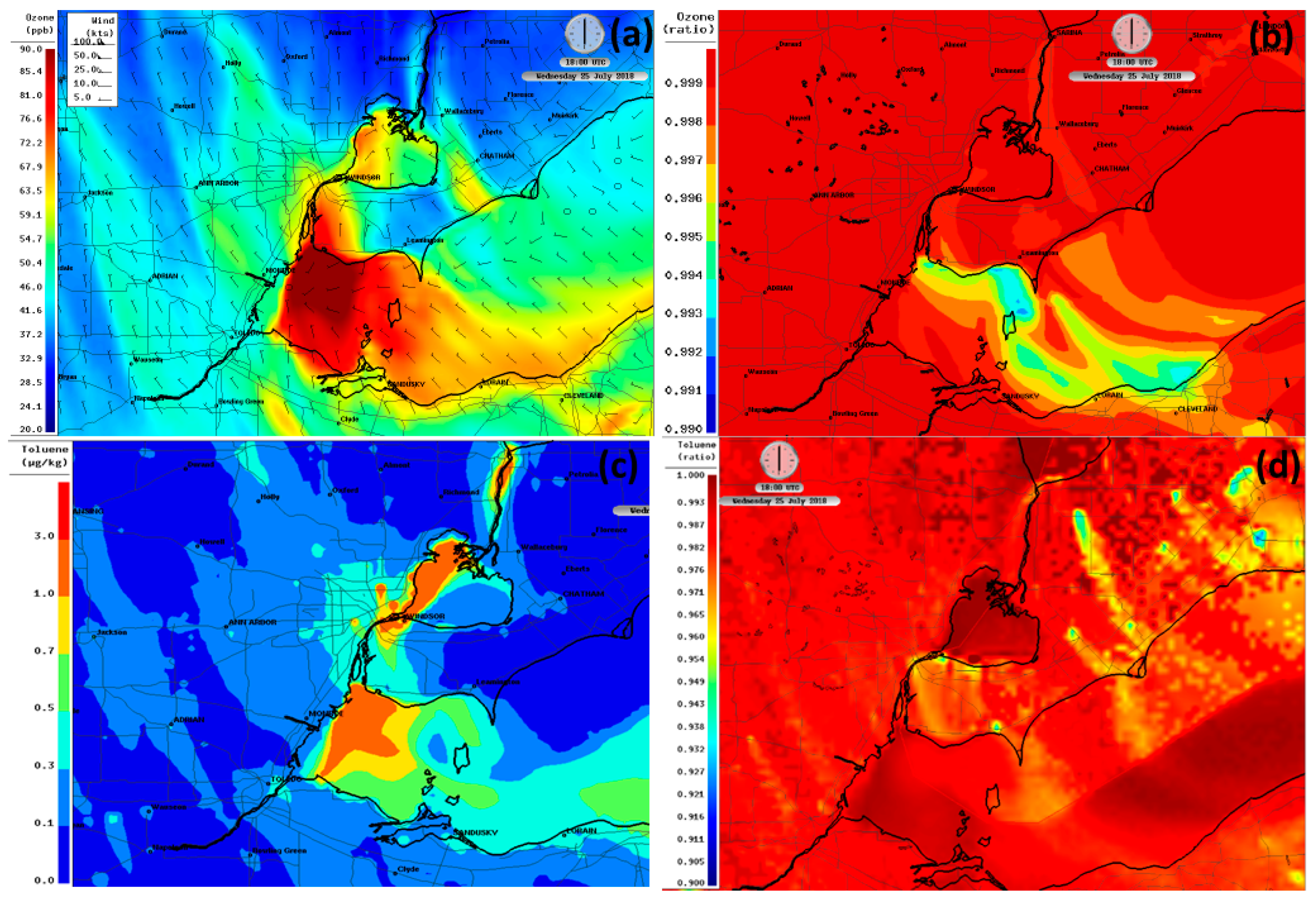
3.8.3. Northwest Flow Pattern

The date 25 July 2018 was chosen as the second case study period. The model predicts O₃ and mono-substituted aromatics reasonably well and at higher-than-average mixing ratios. A simple flow pattern from the northwest was observed and modelled. Higher-than-average loadings on the solvent use factor were noted from positive matrix factorization.

Figure 8a illustrates the modelled O₃ field on 25 July 2018 at 18Z (2 p.m. local). The wind directions were from the northwest of Windsor. The highest O₃ mixing ratios were predicted downwind of Detroit/Windsor, particularly over western Lake Erie, where mixing lengths near the water surface are shallow. The highest mono-aromatic concentrations were detected over Detroit/Windsor/Lake St. Clair, along the St. Clair River, and over Lake Erie. The daytime O₃ ratios were in the range of 0.998–0.999 over Windsor West corresponding to 0.1–0.2% contribution from solvent use applications (Figure 8b). Larger ratios were modelled over Lake Erie due to the westerly flow from Michigan emission sources (e.g., Monroe) and more stable air over the lake. Figure 6 shows that 24 h aromatic concentrations are predicted well (within 10%) compared to observations at Windsor West. Figure 8d illustrates that the aromatic ratios over Windsor were in the range of 0.96–0.97, which corresponds to 30–40% contributions from applications using solvents. Air mass trajectories showed that the air sampled at Windsor West originated over northern Michigan 24 h prior.

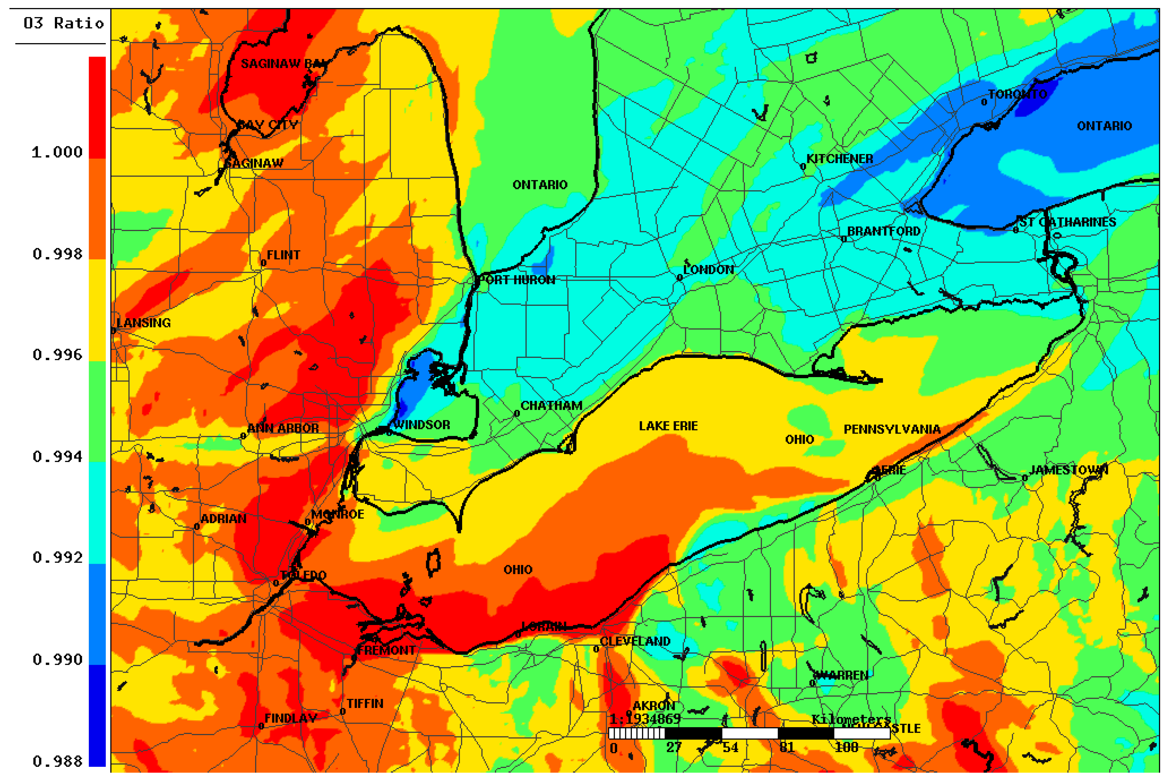
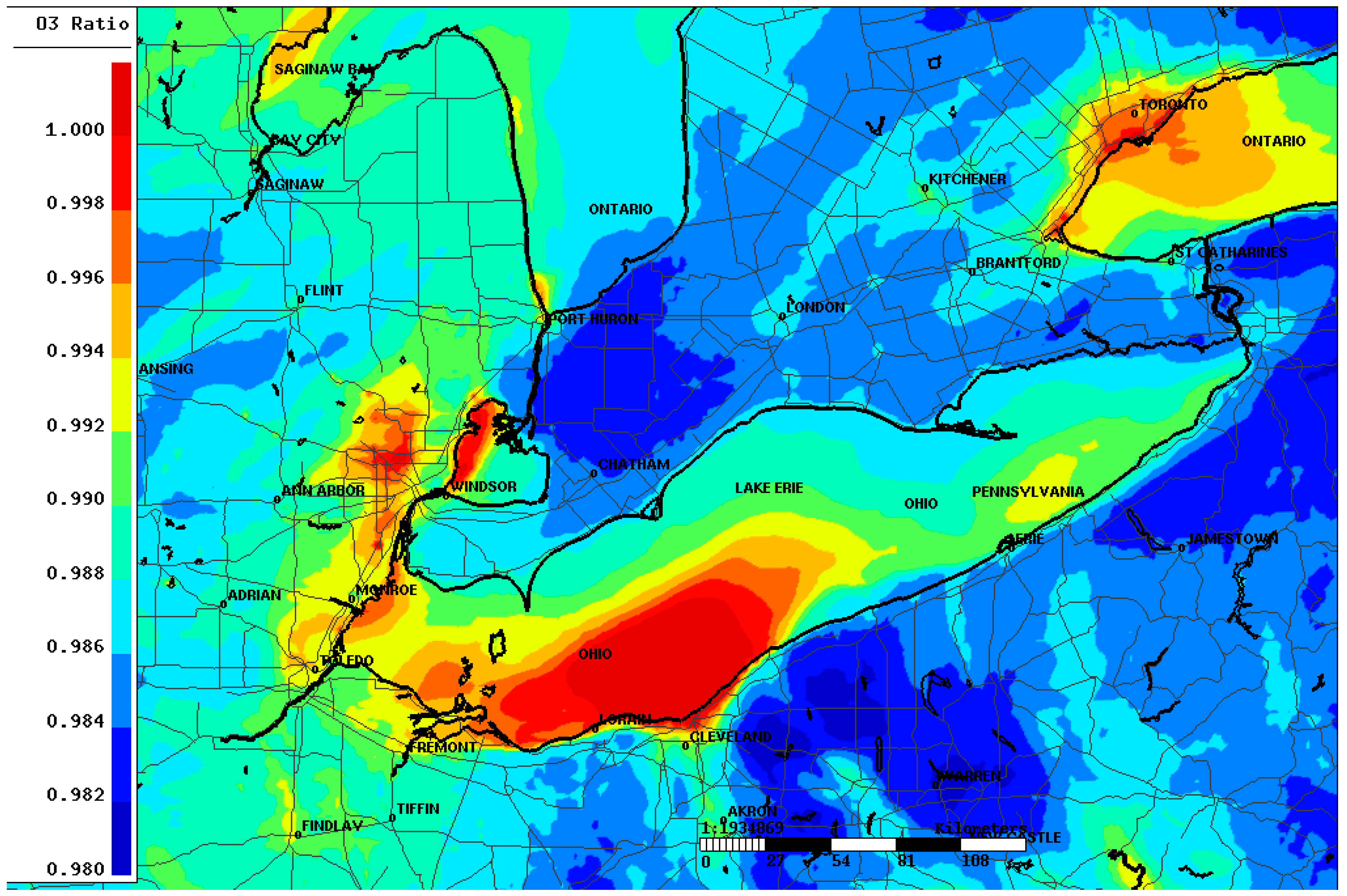
3.9. Impact of 10% Emission Reductions on O₃ for Summertime 2018

Figure 9 shows the average 8 h daytime ratio of the predicted O₃ from the 10% solvent emission reduction simulation relative to the base case simulation. At the Windsor West site, the modelled summertime monthly average O₃ ratio was 0.996, which corresponds to a 0.4% O₃ reduction. The largest O₃ reductions were downwind of the major urban centers, Greater Toronto Area and Detroit/Windsor, in the range of 0.988–0.992, which represents an O₃ decrease of 0.8 to 1.2%. An interesting contrast is observed across the US/Canada border, with generally lower ratios over southern Ontario compared to southern Michigan. This likely reflects the different emission inventory development approaches for the solvent use sub-sectors in the inventories used for the 2018 simulations.

Analysis of emissions in a border domain (Figure S1) showed that on-road and off-road sources are important for NO_x emissions. On the US side, the transportation contribution to NO_x in the border domain was 55%, and in Ontario, the transportation contribution in the border domain was 28%. To assess the O₃ production regime in terms of sensitivity to VOC and NO_x precursors, we performed a summer 2018 simulation with a 10% mobile NO_x emission reduction (both off-road and on-road mobile) and no change to the solvent emissions from the base case. Figure 10 shows the ratio plot for 8 h daily max O₃ for sensitivity divided by the base case, averaged for 2 months in the summer of 2018. Ratios of 0.988 to 0.991 are simulated for Eastern Detroit and Windsor. This represents a 0.8 to 1.1% O₃ decrease. The blue color over rural Michigan and rural Ontario corresponds to a 1.3–1.8% O₃ decrease. The yellow color over Port Huron/Sarnia and Windsor corresponds to a 0.6–0.8% O₃ decrease. Overall, these are larger and more widespread O₃ relative decreases than changes from the solvent use sector alone. This reflects the O₃ production rate sensitivity to NO_x, which is typical of suburban and rural sites in North America.

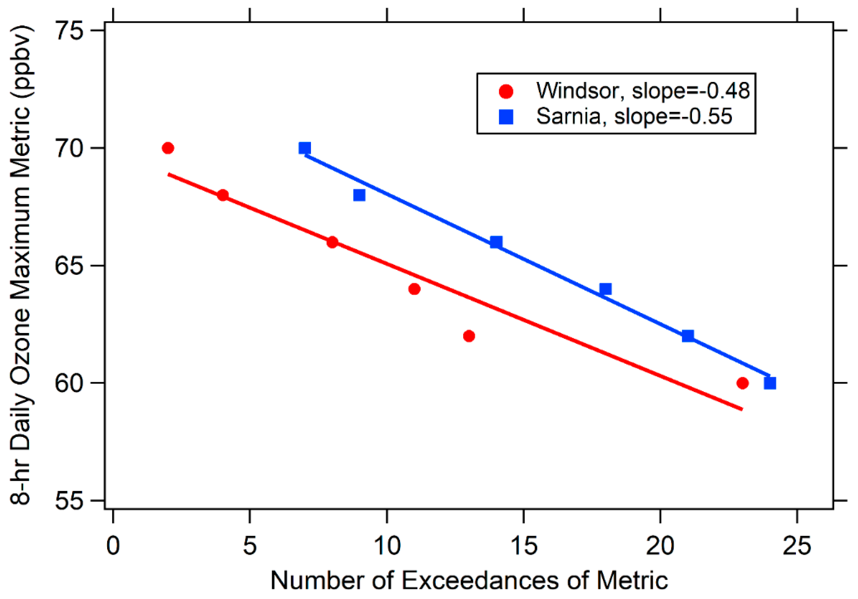
3.10. O₃ Exceedances during MOOSE 2021 at Windsor West and Sarnia, Ontario

Figure 11 illustrates the correlation between the 8 h daily maximum O₃ metric (60 ppbv is the 2025 Canadian standard and 70 ppbv is the current U.S. standard) and the number of exceedances of the metric at the Sarnia and Windsor West stations. Sarnia is an industrial town on the southern shore of Lake Huron across the St. Clair River from Port Huron, Michigan. Sarnia data has a slope of 0.55 ± 0.03 ppbv and the Windsor West data has a slope of 0.48 ± 0.07 ppbv. This means that, on average, lowering the daily maximum O₃ by ~0.5 ppbv or ~0.7% will reduce O₃ exceedances by one year for each of these two cities. This reduction is comparable to the maximum reduction (yellow color) found in the 10% mobile NO_x emission scenario for the Windsor and Sarnia areas (Figure 10).

3.11. Impact of New US Emissions from VCPy Emission Model

Recently, a new framework to model organic emissions from volatile chemical products was developed by the Environmental Protection Agency (EPA) [20]. The model considers both evaporation and product use timescales, and the organic product ingredients are considered individually (i.e., the emission composition is more explicit). This allows for better regional representation and combination of chemical mechanisms. Here, we have processed new solvent emissions using VOC speciation profiles created from the US EPA’s VCPy model [20], as described in Tables S5 and S6.

Figure 12 shows the averaged summer 2021 ratio of the mono-aromatics calculated from the 10% solvent emission reduction relative to the base case. Both simulations used the new US emissions. The significantly higher emissions of solvents within metropolitan Detroit result in ratios of 0.95–0.97, which represents a 35% decrease for mono-aromatics and corresponds to a 30–50% solvent contribution. In addition, a more uniform ratio is now calculated across the Detroit/Windsor border. Other cooler blue spots are also consistent across the domain in both countries. An average ratio of 0.965 is simulated for Windsor West in MOOSE 2021, which represents a 3.5% decrease and an approximate 35% solvent use contribution. This is higher than the 15% contribution at Windsor West for the 2018 summer average and closer to the 44% contribution from the PMF summertime analysis at Windsor West.

It is informative to look at a summer 2021 case study with the new US emissions. Figure 13a illustrates the O₃ surface fields on 20 June 2021 at 18Z. This is a similar southwest wind pattern to the exceedance case on 13 July 2018. A lake breeze forms to the west of Lake St. Clair with the highest O₃ over Detroit along this front. Figure 13b shows the O₃ ratio of the 10% solvent reduction scenario runs relative to the base run. A ratio of 0.994 is simulated, which represents a 0.6% decrease in O₃ for the 10% solvent reduction scenario. Ratios of 0.997 are observed downwind of Detroit over New Haven, which represents a 0.3% reduction. Figure 13c,d show the mono-aromatic concentration and ratio plots. Ratios in light blue over Detroit and downwind correspond to a maximum 6% change and up to 60% contribution from solvent emissions. The O₃ and mono-aromatic sensitivity is higher with these updated US emissions, and gradients across the border between Detroit and Windsor look more reasonable given similar urban population densities.

4. Discussion

This is the first study to describe how solvent emissions from the Canadian air pollutant emission inventory are used in an air quality model and to assess their importance to oxidant air quality in a Canadian city. The 2018 simulations were the first assessment, based on available emission inventories. It should be noted that both the model and measured approaches to estimate source apportionment have uncertainties in source contributions stemming from chemical loss along the air trajectories before reaching the measurement site. The model approach also has uncertainties stemming from the spatial allocation maps used to distribute emissions onto the model grid and the combined VOC speciation used to represent a wide range of chemicals in solvent emissions (e.g., no alcohol species to represent ethanol and alkane used instead due to similar reactivity). The measured concentrations are also 24 h averages and thus capture a range of sources reaching the measurement site. There is also the possibility of volatile chemical products loading on factors for other industrial co-located sources in Detroit and Sarnia. As a result, the modelled and measured source contributions have considerable uncertainties.

The 2021 simulations are built on the 2018 simulations but use updated US emissions from VCPy and a projected Canadian inventory that is closer to the MOOSE study year. The use of the VCPy emission model is a step forward in reducing uncertainties, as it considers the life cycles of consumer products and uses more source-specific speciation profiles (Tables S5 and S6). The VCPy framework is now being used by the ECCC to create future Canadian solvent emissions. Future model development will also improve the model’s VOC speciation to better represent volatile solvent chemicals (e.g., ethanol, glycerol, acetone, limonene, and propylene glycol) and their transformation products. Future field studies in southern Ontario will also use hourly VOC measurements, include more oxygenated VOCs, and measure solvents using source-specific tracer species.

5. Conclusions

The Windsor West PMF results show that solvent use applications are a small emission sector for total VOC (10% by OH-reactivity, 8% by mass) but not insignificant on an annual basis. The 2015 Ontario emission inventory results in an approximate 32% solvent use contribution on an annual basis by mass.

Furthermore, the PMF analysis suggests that approximately 44% of the total mono-aromatics for a summertime average at Windsor West is from solvents used in applications. The contribution was moderately higher on O₃ exceedance days in the summer. The GEM-MACH-TEB model calculates an approximate 30% daytime solvent contribution to the total mono-aromatics for the summertime of 2018 in Windsor. The updated US emissions increase the mono-aromatic solvent contribution to the total mono-aromatics over Windsor/Detroit (30–50%), which is closer to the PMF average solvent factor (44%).

For our 2018 summer simulations, the average 8 h O₃ reduction over Windsor West was 0.4% and smaller over Detroit (0.1–0.3%) from the 10% solvent emission reduction. On average, downwind of Detroit/Windsor over Lake St. Clair, an approximate 1% O₃ decrease was simulated for a 10% solvent emission change. For case studies, downwind of Detroit over the land west of Port Huron, the O₃ change was 0.4–0.6%. For reference, a ~0.7% O₃ change is equivalent to reducing one exceedance event each year in Windsor. For a high O₃ event over Detroit in 2021, the maximum contribution to the total mono-aromatics was 60%, which is considerably higher than the new US emissions. The maximum O₃ change was 0.6% in Detroit, which was also considerably higher than the cases in 2018.

The 10% mobile NO_x reduction scenario resulted in widespread O₃ changes: 0.6–1.1% in Detroit/Windsor and between 1.3 and 1.8% in the rural areas of Southern Ontario. Overall, the results suggest that a solvent reduction scenario would decrease O₃ in the Detroit/Windsor in the urban plume region where O₃ is highest in the mixing ratio (VOC-sensitive O₃ production). A mobile NO_x reduction would decrease O₃ by a similar percentage at Windsor West but also has the benefit of reducing O₃ for suburban and rural locations in the study region (NOx-sensitive O₃ production). A combined emission reduction strategy for Windsor is optimal. This is consistent with the weekend/weekday study by Zhang et al., (2022), which suggests that O₃ production for Windsor is in the transition regime [48].

References

1. Stieb, D.M.; Yao, J.; Henderson, S.B.; Pinault, L.; Smith-Doiron, M.H.; Robichaud, A.; van Donkelaar, A.; Martin, R.V.; Ménard, R.; Brook, J.R. Variability in ambient ozone and fine particle concentrations and population susceptibility among Canadian health regions. Can. J. Public. Health 2019, 110, 149–158. [Google Scholar] [CrossRef] [Green Version]
2. Cohen, A.J.; Brauer, M.; Burnett, R.; Anderson, H.R.; Frostad, J.; Estep, K.; Balakrishnan, K.; Brunekreef, B.; Dandona, L.; Dandona, R.; et al. Estimates and 25-year trends of the global burden of disease attributable to ambient air pollution: An analysis of data from the Global Burden of Diseases Study 2015. Lancet 2017, 389, 1907–1918. [Google Scholar] [CrossRef] [Green Version]
3. Environment and Climate Change Canada. Canadian Environmental Sustainability Indicators: Air Quality. 2023. Available online: www.canada.ca/en/environment-climate-change/services/environmental-indicators/air-quality.html (accessed on 23 April 2023).
4. Foley, T.; Betterton, E.A.; Robert Jacko, P.E.; Hillery, J. Lake Michigan air quality: The 1994–2003 LADCO Aircraft Project (LAP). Atmos. Environ. 2011, 45, 3192–3202. [Google Scholar] [CrossRef]
5. Cleary, P.A.; Fuhrman, N.; Schulz, L.; Schafer, J.; Fillingham, J.; Bootsma, H.; McQueen, J.; Tang, Y.; Langel, T.; McKeen, S.; et al. Ozone distributions over southern Lake Michigan: Comparisons between ferry-based observations, shoreline-based DOAS observations and model forecasts. Atmos. Chem. Phys. 2015, 15, 5109–5122. [Google Scholar] [CrossRef] [Green Version]
6. Goldberg, D.L.; Loughner, C.P.; Tzortziou, M.; Stehr, J.W.; Pickering, K.E.; Marufu, L.T.; Dickerson, R.R. Higher surface ozone concentrations over the Chesapeake Bay than over the adjacent land: Observations and models from the DISCOVER-AQ and CBODAQ campaigns. Atmos. Environ. 2014, 84, 9–19. [Google Scholar] [CrossRef] [Green Version]
7. Brook, J.R.; Makar, P.A.; Sills, D.M.L.; Hayden, K.L.; McLaren, R. Exploring the nature of air quality over southwestern Ontario: Main findings from the Border Air Quality and Meteorology Study. Atmos. Chem. Phys. 2013, 13, 10461–10482. [Google Scholar] [CrossRef] [Green Version]
8. Makar, P.A.; Zhang, J.; Gong, W.; Stroud, C.; Sills, D.; Hayden, K.L.; Brook, J.; Levy, I.; Mihele, C.; Moran, M.D.; et al. Mass tracking for chemical analysis: The causes of ozone formation in southern Ontario during BAQS-Met 2007. Atmos. Chem. Phys. 2010, 10, 11151–11173. [Google Scholar] [CrossRef] [Green Version]
9. McNider, R.T.; Pour-Biazar, A.; Doty, K.; White, A.; Wu, Y.; Qin, M.; Hu, Y.; Odman, T.; Cleary, P.; Kniing, E.; et al. Examination of the physical atmosphere in the Great Lakes region and its potential impact on air quality-Overwater stability and satellite assimilation. J. Appl. Meteor. Climatol. 2018, 57, 2789–2816. [Google Scholar] [CrossRef]
10. Stroud, C.A.; Ren, S.; Zhang, J.; Moran, M.D.; Akingunola, A.; Makar, P.A.; Munoz-Alpizar, R.; Leroyer, S.; Bélair, S.; Sills, D.; et al. Chemical Analysis of Surface-Level Ozone Exceedances during the 2015 Pan American Games. Atmosphere 2020, 11, 572. [Google Scholar] [CrossRef]
11. Foley, K.M.; Pouliot, G.A.; Eyth, A.; Aldridge, M.F.; Allen, C.; Appel, K.W.; Bash, J.O.; Beardsley, M.; Beidler, J.; Choi, D.; et al. 2002–2017 anthropogenic emissions data for air quality modeling over the United States. Data Brief 2023, 47, 109022. [Google Scholar] [CrossRef]
12. Li, W.; Li, L.; Chen, C.-L.; Kacarab, M.; Peng, W.; Price, D.; Xu, J.; Cocker, D.R. Potential of select intermediate-volatility organic compounds and consumer products for secondary organic aerosol and ozone formation under relevant urban conditions. Atmos. Environ. 2018, 178, 109–117. [Google Scholar] [CrossRef] [Green Version]
13. Qin, M.; Murphy, B.N.; Isaacs, K.K.; McDonald, B.C.; Lu, Q.; McKeen, S.A.; Koval, L.; Robinson, A.L.; Efstathiou, C.; Allen, C.; et al. Criteria pollutant impacts of volatile chemical products informed by near-field modelling. Nat. Sustain. 2021, 4, 129–137. [Google Scholar] [CrossRef]
14. Gkatzelis, G.I.; Coggon, M.M.; McDonald, B.C.; Peischl, J.; Aikin, K.C.; Gilman, J.B.; Trainer, M.; Warneke, C. Identifying Volatile Chemical Product Tracer Compounds in U.S. Cities. Environ. Sci. Technol. 2021, 55, 188–199. [Google Scholar] [CrossRef] [PubMed]
15. McDonald, B.C.; Gouw, J.A.D.; Gilman, J.B.; Jathar, S.H.; Akherati, A.; Cappa, C.D.; Jimenez, J.L.; Lee-Taylor, J.; Hayes, P.L.; McKeen, S.A.; et al. Volatile chemical products emerging as largest petrochemical source of urban organic emissions. Science 2018, 359, 760–764. [Google Scholar] [CrossRef] [PubMed] [Green Version]
16. Coggon, M.M.; Gkatzelis, G.I.; McDonald, B.C.; Gilman, J.B.; Schwantes, R.H.; Abuhassan, N.; Aikin, K.C.; Arend, M.F.; Berkoff, T.A.; Brown, S.S.; et al. Volatile chemical product emissions enhance ozone and modulate urban chemistry. Proc. Natl. Acad. Sci. USA 2021, 118, e2026653118. [Google Scholar] [CrossRef]
17. Stroud, C.A.; Zaganescu, C.; Chen, J.; McLinden, C.; Zhang, J.; Wang, D. Toxic volatile organic air pollutants across Canada: Multi-year concentration trends, regional air quality modelling and source apportionment. J. Atmos. Chem. 2016, 73, 137–164. [Google Scholar] [CrossRef] [Green Version]
18. Gkatzelis, G.I.; Coggon, M.M.; McDonald, B.C.; Peischl, J.; Gilman, J.B.; Aikin, K.C.; Robinson, M.A.; Canonaco, F.; Prevot, A.S.H.; Trainer, M.; et al. Observations Confirm that Volatile Chemical Products Are a Major Source of Petrochemical Emissions in U.S. Cities. Environ. Sci. Technol. 2021, 55, 4332–4343. [Google Scholar] [CrossRef]
19. Khare, P.; Gentner, D.R. Considering the future of anthropogenic gas-phase organic compound emissions and the increasing influence of non-combustion sources on urban air quality. Atmos. Chem. Phys. 2018, 18, 5391–5413. [Google Scholar] [CrossRef]
20. Seltzer, K.M.; Pennington, E.; Rao, V.; Murphy, B.N.; Strum, M.; Isaacs, K.K.; Pye, H.O.T. Reactive organic carbon emissions from volatile chemical products. Atmos. Chem. Phys. 2021, 21, 5079–5100. [Google Scholar] [CrossRef]
21. Milbrandt, J.A.; Bélair, S.; Faucher, M.; Vallée, M.; Carrera, M.L.; Glazer, A. The pan-Canadian High Resolution (2.5 km) Deterministic Prediction System. Weather. Forecast. 2016, 31, 1791–1816. [Google Scholar] [CrossRef]
22. Carrera, M.L.; Bélair, S.; Bilodeau, B. The Canadian Land Data Assimilation System (CaLDAS): Description and synthetic evaluation study. J. Hydrometeorol. 2015, 16, 1293–1314. [Google Scholar] [CrossRef]
23. Leroyer, S.; Bélair, S.; Spacek, L.; Gultepe, I. Modelling of radiation-based thermal stress indicators for urban numerical weather prediction. Urban Clim. 2018, 25, 64–81. [Google Scholar] [CrossRef]
24. Ren, S.; Stroud, C.A.; Belair, S.; Leroyer, S.; Munoz-Alpizar, R.; Moran, M.D.; Zhang, J.; Akingunola, A.; Makar, P.A. Impact of Urbanization on the Predictions of Urban Meteorology and Air Pollutants over Four Major North American Cities. Atmosphere 2020, 11, 969. [Google Scholar] [CrossRef]
25. Stroud, C.A.; Morneau, G.; Makar, P.A.; Moran, M.D.; Gong, W.; Pabla, B.; Zhang, J.; Bouchet, V.S.; Fox, D.; Venkatesh, S.; et al. OH-reactivity of volatile organic compounds at urban and rural sites across Canada: Evaluation of air quality model predictions using speciated VOC measurements. Atmos. Environ. 2008, 42, 7746–7756. [Google Scholar] [CrossRef]
26. Stockwell, W.R.; Lurmann, F.W. Intercomparison of the ADOM and RADM Gas-Phase Chemical Mechanisms; Electrical Power Research Institute Topical Report; EPRI: Palo Alto, CA, USA, 1989; p. 254. [Google Scholar]
27. Stockwell, W.R. The effect of gas-phase chemistry on aqueous-phase sulfur dioxide oxidation rates. J. Atmos. Chem. 1994, 19, 317–329. [Google Scholar] [CrossRef]
28. Sassi, M.; Zhang, J.; Moran, M.D. SMOKE-Ready Canadian Air Pollutant Emission Inventory (APEI) Package version 1 [Data Set], Zenodo. 2021. Available online: https://zenodo.org/record/4883639 (accessed on 14 March 2023).
29. Environment and Climate Change Canada (ECCC). National Air Pollution Surveillance (NAPS) Program. 2023. Available online: https://donnees-data.ec.gc.ca/data/air/monitor/national-air-pollution-surveillance-naps-program (accessed on 14 March 2023).
30. United States Environmental Protection Agency (USEPA). EPA Positive Matrix Factorization (PMF) 5.0 Fundamentals and User Guide. 2014. Available online: https://www.epa.gov/sites/default/files/2015-02/documents/pmf_5.0_user_guide.pdf (accessed on 14 March 2022).
31. Li, Z.; Ho, K.F.; Yim, S.H.L. Source apportionment of hourly-resolved ambient volatile organic compounds: Influence of temporal resolution. Sci. Total. Environ. 2020, 725, 138243. [Google Scholar] [CrossRef]
32. Baudic, A.; Gros, V.; Sauvage, S.; Locoge, N.; Sanchez, O.; Sarda-Estève, R.; Kalogridis, C.; Petit, J.-E.; Bonnaire, N.; Baisnée, D.; et al. Seasonal variability and source apportionment of volatile organic compounds (VOCs) in the Paris megacity (France). Atmos. Chem. Phys. 2016, 16, 11961–11989. [Google Scholar] [CrossRef] [Green Version]
33. Wang, L.; Xiang, Z.; Stevanovic, S.; Ristovski, Z.; Salimi, F.; Gao, J.; Wang, H.; Li, L. Role of Chinese cooking emissions on ambient air quality and human health. Sci. Total. Environ. 2017, 589, 173–181. [Google Scholar] [CrossRef]
34. Pengchuan, L.; Gao, J.; Xu, Y.; Schauer, J.; Wang, J.; He, W.; Nie, L. Enhanced commercial cooking inventories from the city scale through normalized emission factor dataset and big data. Environ. Pollut. 2022, 315, 120320. [Google Scholar] [CrossRef]
35. Li, Z. Long Term Trend and Source Apportionment of Ambient VOCs in Windsor. Master’s Thesis, University of Windsor, Windsor, ON, Canada, 2013. Available online: https://scholar.uwindsor.ca/etd/4984 (accessed on 2 January 2023).
36. Carter, W.P.L. Development of the SAPRC-07 Chemical Mechanism and Updated Ozone Reactivity Scales. Contracts No. 03-318, 06-408, and 07-730, Riverside: Center for Environmental Research and Technology, College of Engineering, University of California. 2010. Available online: https://intra.engr.ucr.edu/~carter/SAPRC/saprc07.pdf (accessed on 3 November 2022).
37. Heimann, G.; Warneck, P. Hydroxyl radical-induced oxidation of 2,3-dimethylbutane in air. J. Phys. Chem. 1992, 96, 8403–8409. [Google Scholar] [CrossRef]
38. Iuga, C.; Osnaya-Soto, L.; Ortiz, E.; Vivier-Bunge, A. Atmospheric oxidation of methyl and ethyl tert-butyl ethers initiated by hydroxyl radicals. A quantum chemistry study. Fuel 2015, 159, 269–279. [Google Scholar] [CrossRef]
39. Orkin, V.L.; Khamaganov, V.G.; Kozlov, S.N.; Kurylo, M.J. Measurements of rate constants for the OH reactions with bromoform (CHBr3), CHBr2Cl, CHBrCl2, and epichlorohydrin (C3H5ClO). J. Phys. Chem. A 2013, 117, 3809–3818. [Google Scholar] [CrossRef] [PubMed]
40. Permar, W.; Jin, L.; Peng, Q.; O’Dell, K.; Lill, E.; Selimovic, V.; Selimovic, V.; Yokelson, R.J.; Hornbrook, R.S.; Hills, A.J.; et al. Atmospheric OH reactivity in the western United States determined from comprehensive gas-phase measurements during WE-CAN. Environ. Sci. Atmos. 2023, 3, 97–114. [Google Scholar] [CrossRef]
41. Yu, S.; Mathur, R.; Schere, K.; Kang, D.; Pleim, J.; Otte, T.L. A detailed evaluation of the Eta-CMAQ forecast model performance for O3, its related precursors, and meteorological parameters during the 2004 ICARTT study. J. Geophys. Res. Atmos. 2007, 112, D12. [Google Scholar] [CrossRef] [Green Version]
42. Dennis, R.; Fox, T.; Fuentes, M.; Gilliland, A.; Hanna, S.; Hogrefe, C.; Irwin, J.; Rao, S.T.; Scheffe, R.; Schere, K.; et al. A framework for evaluating regional-scale numerical photochemical modeling systems. Environ. Fluid Mech. 2010, 10, 471–489. [Google Scholar] [CrossRef] [Green Version]
43. Rao, S.T.; Galmarini, S.; Puckett, K. Air quality model evaluation international initiative (AQMEII): Advancing the state of the science in regional photochemical modeling and its alication. Bull. Am. Meteorol. Soc. 2011, 92, 23–30. [Google Scholar] [CrossRef] [Green Version]
44. Simon, H.; Baker, K.R.; Phillips, S. Compilation and interpretation of photochemical model performance statistics published between 2006 and 2012. Atmos. Environ. 2012, 61, 124–139. [Google Scholar] [CrossRef]
45. Baker, K.; Liljegren, J.; Valin, L.; Judd, L.; Szykman, J.; Millet, D.; Czarnetzki, A.; Whitehill, A.; Murphy, B.; Stanier, C. Photochemical model representation of ozone and precursors during the 2017 Lake Michigan ozone study (LMOS). Atmos. Environ. 2023, 293, 119465. [Google Scholar] [CrossRef]
46. Thunis, P.; Clappier, A.; Tarrason, L.; Cuvelier, C.; Monteiro, A.; Pisoni, E.; Wesseling, J.; Belis, C.A.; Pirovano, G.; Janssen, S.; et al. Source apportionment to support air quality planning: Strengths and weaknesses of existing approaches. Environ. Int. 2019, 130, 104825. [Google Scholar] [CrossRef]
47. Zhang, T.; Xu, X.; Su, Y. Impacts of Regional Transport and Meteorology on Ground-Level Ozone in Windsor, Canada. Atmosphere 2020, 11, 1111. [Google Scholar] [CrossRef]
48. Zhang, T.; Xiaohong, X.; Yushan, S. Long-term measurements of ground-level ozone in Windsor, Canada and surrounding areas. Chemosphere 2022, 294, 133636. [Google Scholar] [CrossRef] [PubMed]
Figure 1. Study methodology linking emissions processing (green font), air quality model (red font), ambient measurements, and analysis (black font).
Atmosphere 14 01094 g001
Figure 2. Population density in the study region. Cities and towns are marked for reference.
Atmosphere 14 01094 g002
Figure 3. PMF factor identification by mass percentage (a) and OH-reactivity weighted mole percentage (b) from 2018 annual data at Windsor West. Solvent usage contributions of 8% and 10% are calculated by mass and reactivity-weighted, respectively. The reactivity-weighted factors are more evenly distributed.
Atmosphere 14 01094 g003
Figure 4. Correlation between the 8 h daily maximum modelled ozone and 8 h daily maximum measured ozone at Windsor West for June and July 2018.
Atmosphere 14 01094 g004
Figure 5. The ratio of 8 h daytime mono-substituted aromatic concentration from the sensitivity run to the base case simulation (average for June and July 2018). The sensitivity run used a 10% solvent use application for VOC emission reduction. The average 8 h daytime aromatic ratio at Windsor West is 0.97 (3% decrease), which represents an approximate 30% contribution from solvent use and coating emissions. Blue color represents ratios of 0.93 (7% decrease) in industrial areas. The dot shows the location of the Windsor West NAPS site.
Atmosphere 14 01094 g005
Figure 6. The 8 h daytime ozone maximum and 24 h mono-substituted aromatics time series at Windsor West. As case study periods, 13 July and 25 July were selected due to good model and measurement agreement and contrast in meteorology and pollutant concentrations.
Atmosphere 14 01094 g006
Figure 7. (a) Ozone and wind barbs predicted on 13 July 2018 at 20Z, (b) ozone ratio predicted from the 10% emission reduction simulation relative to the base simulation, (c) mono-aromatic concentration predicted, and (d) mono-aromatic ratio predicted from the 10% emission reduction simulation relative to the base simulation. Downwind of Windsor/Detroit, the ozone ratios were from 0.994 to 0.996 (0.4–0.6% reduction) on the eastern side of the ozone plume near Port Huron. The lowest ratios in Detroit (0.996 to 0.998) were also found along the lake breeze front to the west of Lake St. Clair (0.2–0.4% decrease). Mono-aromatic ratios of 0.97 to 0.99 were simulated in the Detroit/Windsor and downwind plumes, which represents a small 1–3% decrease.
Atmosphere 14 01094 g007
Figure 8. (a) Ozone predicted at the surface on 25 July 2018 at 18Z, (b) ratio of ozone from 10% solvent use reduction scenario relative to the base case, (c) mono-aromatic concentration predicted, and (d) ratio of mono-aromatic from the 10% solvent use reduction scenario relative to the base case. Daytime ozone ratios were in the range of 0.998–0.999 over Windsor West corresponding to 0.1–0.2% contribution from solvent use. Larger ratios were modelled over Lake Erie due to the westerly flow from Michigan emission sources (e.g., Monroe) and more stable air over the lake. Mono-aromatic ratios over Windsor were in the range of 0.96–0.97, which corresponds to a 3–4% decrease.
Atmosphere 14 01094 g008
Figure 9. Average summertime 8 h daytime ratio of the predicted ozone from the 10% solvent emission reduction simulation relative to the base case simulation. At the Windsor West site, the average ratio was 0.996, which corresponds to a 0.4% ozone reduction. The largest ozone reductions were downwind of the major urban centers, Toronto and Detroit/Windsor, in the range of 0.988–0.992, which represents an ozone decrease of 0.8 to 1.2%.
Atmosphere 14 01094 g009
Figure 10. Average summertime 8 h daytime ratio of the predicted ozone from the 10% mobile emission reduction simulation relative to the base case simulation. Low ratios of 0.988 to 0.991 are simulated for Eastern Detroit (0.8 to 1.1% decrease, green). The blue color over rural Michigan and rural Ontario corresponds to a 1.3–1.8% ozone decrease. The yellow color over Port Huron/Sarnia and Windsor corresponds to a 0.6–0.8% ozone decrease. Western Detroit, Toronto, and pollution plumes over the lakes have small ozone decreases shown in red.
Atmosphere 14 01094 g010
Figure 11. Correlation between the 8 h daily maximum ozone (in ppbv) and the number of exceedances of this metric at both Windsor West and Sarnia, Ontario. The slope (−0.5 ppbv) represents the average reduction in ozone (ppbv) needed to decrease the number of exceedance events by 1.
Atmosphere 14 01094 g011
Figure 12. Ratio of summertime 8 h daytime mono-aromatic mixing ratio from the 10% sensitivity run relative to the base case simulation (average for June and July 2021). The sensitivity run used a 10% VOC solvent use application emission reduction. Within metropolitan Detroit, ratios of 0.95–0.97 are modelled, which represents a 3–5% decrease. An average ratio of 0.965 is simulated for Windsor West, which represents a 3.5% decrease. In addition, a more uniform ratio is now calculated across the Detroit/Windsor border. US emissions are calculated with the VCPy method.
Atmosphere 14 01094 g012
Figure 13. (a) Ozone surface field predicted on 20 June 2021 at 18Z, (b) ozone ratio from 10% solvent reduction simulation relative to base case run, (c) mono-aromatic concentration predicted, (d) mono-aromatic ratio from 10% solvent use reduction simulation relative to base case run. An ozone ratio of 0.994 is simulated over Eastern Detroit, which represents a 0.6% decrease. Ratios of 0.997 are observed downwind of Detroit over New Haven, which represents a 0.3% decrease. Mono-aromatic ratios in light blue over Detroit and downwind correspond to a maximum 6% decrease.
Atmosphere 14 01094 g013