On the Variability of In Situ Surface Layer Refractivity Measurements

Abstract

Direct measurements of profiles of atmospheric properties near the ocean surface and within the marine atmospheric surface layer often contain a large degree of variability. The variability observed can be explained by numerous technical and natural reasons such as the temporal variability over the time span a profile is measured (unsteadiness in the mean), spatial variations (inhomogeneity), turbulent fluctuations, and measurement uncertainty. In this study, we explored the observed variability in vertical distributions of refractive index measured with a tethered-balloon-based marine atmospheric profiling system (MAPS). MAPS profiled the atmosphere from approximately 0.5 to 50 m, with instantaneous (order 1 s) measurements performed at each profiled altitude. To explore whether the observed scatter could be largely explained by (inertial-scale) turbulent fluctuations, we simulated refractive index fluctuations with a spectral-based turbulent refractive index fluctuation (TRIF) model. TRIF was optimized based on the MAPS measurements to determine a vertical length scale of the turbulence. The scales computed in the optimization were reasonable based on other estimates in the literature under similar conditions. However, finer-scale trends of the length scale with atmospheric stability did not match expectations, and thus the estimated length scales may be considered more as an order-of-magnitude estimate rather than an exact measurement of this scale. The ability to match the observed variability in the MAPS data using a turbulence model with a reasonable choice of vertical length scale suggests that the MAPS variability is dominated by physical processes such as turbulence rather than being primarily driven by measurement uncertainty.

1. Introduction

Exchanges of momentum, heat, and water vapor between the ocean and atmosphere have been the focal point of extensive research. Air–sea interaction, partly described by turbulent exchanges, plays a significant role in the forecasting of not only maritime weather but also global climate. The study of these exchanges is generally located within the first 100 m, a region known as the marine atmospheric surface layer (MASL). Turbulent exchanges, measured as fluxes of momentum, heat, and water vapor, have been the focus of multiple major field campaigns in recent decades. Specifically, the notorious Kansas experiments [1,2], which were performed over land, have been the foundation of statistical relationships relating surface fluxes to the mean vertical distributions of wind, temperature, and humidity within the atmospheric surface layer.

Experiments analogous to the Kansas experiments have been performed in the MASL, where one of the most prominent is the tropical ocean–global atmosphere (TOGA) campaign [3,4]. The goal of TOGA was to identify and understand the physical processes coupling the ocean and atmosphere and describe how the coupled effects of buoyancy and wind forcing drive variations in distributions of meteorological parameters (i.e., temperature, wind, and humidity). These field experiments inspired the coupled ocean–atmosphere response experiment (COARE) [4,5], which estimated air–sea fluxes from bulk variables employing Monin–Obukhov (MO) similarity theory (MOST). COARE continues to be one of the most popular surface layer estimation algorithms, and [5] discusses updates to the algorithm, specifically the universal stability functions.

Similar to COARE, the Navy Atmospheric Vertical Surface Layer Model (NAVSLaM) estimates surface layer fluxes and related vertical distributions of meteorological parameters [6]. NAVSLaM is blended with a numerical weather prediction (NWP) model, the Coupled Ocean–Atmosphere Mesoscale Prediction System (COAMPS^®) [7], to comprehensively forecast the MASL. The novelty of NAVSLaM, relative to COARE, is the dynamic application of stability functions, where unstable regimes employ Businger–Dyer stability functions [1], and stable regimes employ modified Grachev functions [8]. This dynamic use of stability functions presumably leads to a more accurate estimation of surface layer fluxes and, thus, more accurate estimates of vertical distributions of meteorological parameters [6]. While these models strive to capture the impact of turbulent fluctuations on the time-averaged vertical profiles of wind, temperature, and humidity, they are unable to predict instantaneous realizations of turbulent fields. Such realizations from first physical principles require complex numerical frameworks such as large eddy simulation (LES) of the air–sea interface [9].

To measure turbulent fluctuations directly requires high temporal and spatial resolution. An example of such a measurement system is the marine atmospheric profiling system (MAPS), pioneered by [10], which was designed to obtain independent measurements of temperature and humidity at multiple vertical levels within the first 50 m of the MASL. Each measurement, sampled at 1 Hz, as a tethered radiosonde is rapidly winched up and down over the lower 50 m of altitude, captures the instantaneous air property at each time and location. MAPS was extensively deployed during the Coupled Air–Sea Processes and Electromagnetic Ducting Research (CASPER) East and West campaigns [11,12], and multiple studies have incorporated this data, demonstrating its exceptional quality [13,14,15,16,17]. The MAPS measurements show a high degree of variability in space and time [10,16], which could be explained by, for example, turbulent fluctuations and/or measurement uncertainty. The latter would be random while the former only pseudo-random.

To model refractive index fluctuations, spectral modeling has been employed within the MASL. Prior studies have utilized statistical methods to describe turbulent fluctuations of refractivity where the most common approach is the use of the Kolmogorov spectrum [18,19,20,21,22]. This spectrum is a function of the refractive index structure constant ($C_n^2$) and the outer length scale ($L_o$) of turbulence, where $C_n^2$ is a parameter relating to the magnitude of turbulent fluctuations, and $L_o$ delineates the length scale of the energy containing or “mixing” threshold of the inertial subrange.

The current study aimed to explore the MAPS measurements, specifically the variations captured by the system, over the course of the CASPER-East campaign. To investigate whether measurement variations can be explained by turbulent fluctuations, turbulent refractive index fluctuations were simulated using a 1-D anisotropic Kolmogorov spectral model, referred to as the TRIF model. Particle swarm optimization (PSO) was utilized to optimize the TRIF model to the measurements, specifically the outer vertical length scale, $L_z$, was derived via PSO for $C_n^2$ estimated from CASPER-East data via NAVSLaM. Comparisons of (i) MAPS and TRIF model fluctuations and (ii) derived $L_z$ and previously reported estimations of surface layer $L_z$ give insight into whether refractive index variability observed in MAPS refractivity could be physically explained by turbulent fluctuations. Furthermore, an ability to replicate the MAPS data variability also partly validates the TRIF modeling approach.

The following sections are organized as follows: Section 2 discusses the CASPER-East meteorological data, highlighting the MAPS dataset, Section 3 describes the TRIF model, and Section 4 discusses the optimization method. Section 5 presents the results of the optimization experiment and associated discussion of the results, followed by a concluding Section 6.

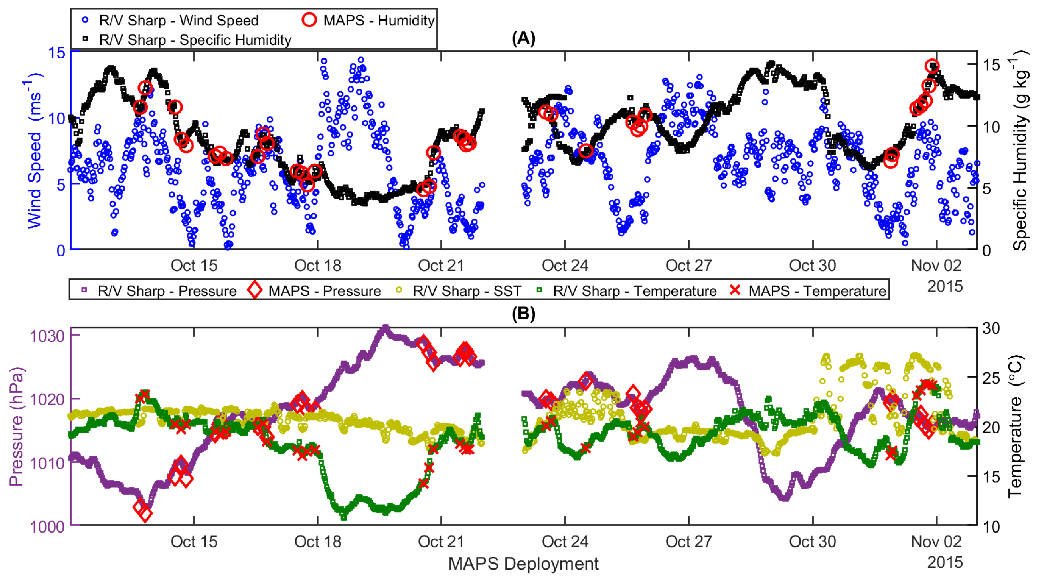
2. CASPER-East Measurements

The CASPER-East field campaign occurred over 25 days in 2015 between 12 October and 6 November [11]. The following paragraphs describe the measurements made within the MASL by MAPS and aboard the Research Vessel (R/V) Sharp. Comprehensive discussion of the CASPER-East campaign can be found in [11].

The MAPS system was constructed of an iMET rawinsonde attached to a balloon tethered to a small workboat, using a winch to control the ascent and decent of the system from ~0.5 m to ~50 m in altitude. The workboat used to deploy MAPS was small enough that its effects on the measured environment are considered minimal [10]. Pressure, temperature, and relative humidity accuracies were 0.5 hPa, 0.2 °C, and 5%, respectively, with resolutions of approximately one-tenth of their accuracy for each. Response times for all sensors were below 2 s. MAPS datasets were composed of pressure (p), temperature (T), and relative humidity (RH), where T and RH were converted to potential temperature (θ) and specific humidity (q), respectively. In [10], T, q, and p data were fit with a 7th-order polynomial for each MAPS dataset; the instantaneous measurements along with these fits were used in this study. Time series of meteorological variables at 12 m altitude are illustrated in Figure 1 along with bulk meteorological measurements (30 min averages) made aboard the R/V Sharp (note that the time series gap is due to a port call mid-cruise). Vertical profiles of modified refractivity ($M$) were computed from the mean meteorological profiles via [23]:

$$M=\frac{77.6}{T}\left[p+\frac{4810e}{T}\right]+\left(\frac{z}{a}\right)\times {10}^6,$$

(1)

where $z$ is the height above the earth’s surface, $a$ is the radius of the earth, and $e$ is the partial water vapor pressure (millibars) computed with q and T to estimate the saturation vapor pressure [24]. The polynomial fits of mean p, T, and RH were based on data measured down to ~0.5 m; thus, the polynomial fit was also used to extrapolate M to the surface to obtain surface refractivity ($M_0$). Previous studies found that this 7th-order polynomial represents near-surface variations that are more consistent with MOST surface layer model predictions than lower-order polynomial fits, and it also results in a smoother vertical refractivity profile than using a method such as bin-averaging the data over altitude (Figure 2). A more extensive discussion of this methodology can be found in [13,14].

MAPS measurements of p, T, and RH have been thoroughly verified [10,12,13,14]. This paper focuses on the modified refractivity estimated from these measurements. MAPS datasets used in this study are displayed in

Table 1. Overview of MAPS datasets. Dataset number, deployment time, deployment duration, number of launches, number of samples, and root mean squared (RMS) fluctuation of the MAPS measurements over each deployment are shown. Also included are the NAVSLaM estimated refractive index structure constant ($C_n^2$), optimized vertical outer length scale ($L_z$), and corresponding fitness score (${\mathsf{\Omega }}_{Fit}$), defined in (10), evaluated for each optimization.

MAPS Dataset	Deployment Time (EST)	Duration (min.)	Launches	Samples	M′ RMS (M-Units)	NAVSLaM ${\mathit{C}}_{\mathit{n}}^{\mathbf{2}}$ (m−2/3)	Derived Lz (m)	ΩFIT (M-Units2)
1	13-Oct 12:49	22	7	1572	1.092	4.75 × 10−13	4.69	0.010
2	13-Oct 15:47	25	7	1264	1.021	4.96 × 10−13	4.24	0.001
3	14-Oct 09:06	19	5	698	1.471	4.66 × 10−13	5.89	0.035
4	14-Oct 12:42	38	7	867	1.742	3.22 × 10−13	8.09	0.022
5	14-Oct 15:32	17	6	684	1.442	8.34 × 10−13	4.51	0.022
6	15-Oct 08:22	9	7	936	1.799	1.35 × 10−12	4.58	0.095
7	15-Oct 11:03	54	6	981	1.835	1.17 × 10−12	4.74	0.081
8	15-Oct 14:41	30	6	737	1.350	1.01 × 10−12	4.08	0.019
9	16-Oct 09:12	44	2	364	1.580	1.73 × 10−12	3.81	0.009
10	16-Oct 12:16	20	6	1077	1.664	1.79 × 10−12	3.70	0.024
11	16-Oct 14:38	32	7	1134	2.186	1.27 × 10−12	5.51	0.036
12	17-Oct 08:07	22	9	945	1.216	1.48 × 10−12	3.19	0.035
13	17-Oct 11:04	14	7	1250	1.837	1.09 × 10−12	5.01	0.091
14	17-Oct 14:06	16	7	873	1.481	1.23 × 10−12	3.91	0.034
15	17-Oct 18:25	35	3	295	1.164	9.47 × 10−13	3.58	0.092
16	20-Oct 09:41	32	20	2643	1.427	7.06 × 10−13	4.93	0.016
17	20-Oct 12:57	23	10	1585	1.968	7.56 × 10−13	5.87	0.060
18	20-Oct 15:29	45	15	2287	1.749	6.74 × 10−13	5.70	0.020
19	21-Oct 07:01	41	7	969	1.605	1.95 × 10−13	9.42	0.125
20	21-Oct 08:57	34	8	859	1.116	2.20 × 10−13	6.42	0.059
21	21-Oct 10:29	17	7	619	1.094	5.30 × 10−13	4.73	0.010
22	21-Oct 12:10	42	7	695	1.252	3.09 × 10−13	5.85	0.030
23	23-Oct 08:43	22	14	1837	1.991	1.67 × 10−13	11.80	0.021
24	23-Oct 11:44	18	9	1457	2.253	1.66 × 10−13	13.57	0.061
25	24-Oct 08:05	31	6	920	2.290	1.81 × 10−12	4.85	0.086
26	25-Oct 11:25	30	16	2072	1.870	4.43 × 10−13	7.59	0.011
27	25-Oct 14:11	25	14	1892	1.190	2.98 × 10−14	17.02	0.002
28	25-Oct 15:58	24	8	1187	0.955	3.44 × 10−13	4.68	0.005
29	25-Oct 18:28	37	6	748	0.749	3.99 × 10−13	3.98	0.010
30	31-Oct 17:19	25	8	799	0.958	9.96 × 10−13	2.96	0.007
31	31-Oct 18:15	30	7	850	1.838	1.09 × 10−12	4.85	0.072
32	01-Oct 08:31	21	10	1533	2.770	1.98 × 10−12	5.38	0.127
33	01-Oct 10:57	19	10	1570	3.076	1.36 × 10−12	7.07	0.260
34	01-Oct 13:30	28	8	1306	2.601	2.52 × 10−12	4.75	0.065
35	01-Oct 15:39	19	7	1226	2.390	2.16 × 10−12	4.78	0.019
36	01-Oct 17:32	11	12	967	1.183	1.64 × 10−12	3.02	0.002

, showing that 36 deployments of the system were performed over the course of CASPER-East, and on average each deployment lasted 26 min and contained ~1158 samples. Numerous ascents and subsequent descents of MAPS occurred during each deployment, where the following use of the term “launch” will describe one ascent/descent of the system, each lasting on average ~3.5 min. For each MAPS deployment, multiple launches occurred. For this study, MAPS refractivity estimates were truncated above 50 m to remove measurement uncertainties occurring due to reorientation of the system from ascent to descent [13,14]. In Figure 2, 4 example deployments of MAPS from CASPER-East are illustrated, where the different marker colors indicate different launches of MAPS; the 7th-order polynomial fit represents the mean; and, for comparison, a 1 m altitudinally binned mean profile is shown for each dataset, with the former utilized as the mean profile in this study. MAPS measurements, and subsequent estimates of refractivity, individually can be considered instantaneous (within the longest response time of the sensors of <2 s) and can thus be decomposed as

$$M\left(z\right)=\bar{M}\left(z\right)+M^{\prime }\left(z\right),$$

(2)

where the overbar and prime denote a mean and fluctuation, respectively. In Figure 2, instantaneous MAPS-based $M$ are shown as markers, and the 7th-order polynomial fits, representing the mean of the markers, is shown as a black line ($\bar{M}$). Refractive index fluctuations ($M^{\prime }$) computed from (2) are illustrated in Figure 3. The mean $M^{\prime }$ for each MAPS dataset is approximately zero, as exemplified in Figure 3 for the same datasets shown in Figure 2. The zero means of $M^{\prime }$ confirm that the polynomial fits are reasonable estimates of $\bar{M}$.

In conjunction with the MAPS deployments, meteorological and sea surface measurements were conducted aboard the R/V Sharp. Wind speed was not measured by MAPS and is needed for estimation of $C_n^2$, discussed in Section 3.2; thus, wind speed was obtained from an anemometer aboard the R/V Sharp bow mast (z = 12 m) averaged over 30 min intervals. Skin sea surface temperature (SST) was also measured aboard the R/V Sharp, corrected from the 5 min bulk SST [11,16]. Time series of R/V Sharp SST and wind speed are displayed in Figure 1.

3. Turbulent Refractive Index Fluctuations Model (TRIF)

Previous studies have modeled turbulent refractive index fluctuations using a variety of models for representing turbulence—such as Gaussian, von Karman, and Kolmogorov-based spectral models [18,19,20,21,22]. Because a Kolmogorov-based spectral model only emulates turbulence in the inertial subrange, it is easier to incorporate anisotropy into the model, which is a key characteristic of turbulence in the MASL. Therefore, an anisotropic Kolmogorov-based turbulent refractive index fluctuation model (TRIF) was implemented in this study [19]. Details of the implementation of this Kolmogorov model are discussed in Section 3.1, where it is revealed that a refractive index structure constant is needed for the model. The method for estimating this structure constant is described in Section 3.2.

3.1. Spectral Modeling of Tubulent Refractive Index Fluctuations

Refractivity was assumed to be constantly perturbed by continuous fluctuations due to atmospheric turbulence. Random fluctuations, as defined in (2), were modeled stochastically. The stochastic fluctuating component of the index of refraction (IOR) is described by the Kolmogorov spectrum derived by [25]:

$$\varnothing \left(\mathit{k}\right)=\frac{0.033C_n^2}{{\left(L_0^{-2}+{\mathit{k}}^2\right)}^{\frac{11}{6}}},$$

(3)

where $C_n^2$ is in units of m^−2/3, $L_0$ has units of meters, and $\mathit{k}$ is the 3-dimensional wavenumber vector. The anisotropic MASL can be introduced into (3) via $\alpha$, a parameter describing the relationship between horizontal ($L_x)$ and vertical ($L_z$) outer length scales, where $L_z=\alpha L_x$ [18,20,22]; thus:

$$\varnothing \left({\kappa }_x,{\kappa }_y,{\kappa }_z\right)=\frac{0.033C_n^2}{{\left(L_x^{-2}+{\kappa }_x^2+{\kappa }_y^2+{\alpha }^2{\kappa }_z^2\right)}^{\frac{11}{6}}}$$

(4)

For this study, $\alpha$ = 0.27 [26]. To collapse the three-dimensional spectrum in (4) into one-dimensional space, the transverse vertical spectrum was adopted as derived in [18,20]:

$$S_n\left({\kappa }_z\right)={\left(2\pi \right)}^2\delta x\underset{-\infty }{\overset{+\infty }{\int }}\varnothing \left({\kappa }_x=0,{\kappa }_y,{\kappa }_z\right)d{\kappa }_y,$$

(5)

where $\delta x$ is a scaling factor that would account for the distance between realizations of vertical turbulent profiles in a numerical model. In the present study, we were not generating realizations within a numerical model but rather comparing a single vertical refractive index fluctuation realization to each MAPS dataset, so no scaling was required; thus, we simplify $\delta x=1$ in (5). Substituting (5) into (4) results in the one-dimensional transverse spectrum:

$$S_n\left({\kappa }_z\right)={\left(2\pi \right)}^2\frac{\Gamma \left(\frac{1}{2}\right)\Gamma \left(\frac{4}{3}\right)}{\Gamma \left(\frac{11}{6}\right)}{\alpha }^{-\frac{8}{3}}\frac{0.033C_n^2}{{\left(L_z^{-2}+{\kappa }_z^2\right)}^{\frac{4}{3}}},$$

(6)

where $\Gamma$ is a gamma function. The full derivation of (6) can be found in [18,20,22]. Realizations of refractive index fluctuations from $S_n\left({\kappa }_z\right)$ are found using the approximate frequency domain method proposed in [27] and similarly implemented in [22]. Realized refractive index fluctuations are related to modified refractivity by

$$M=\left(n-1+\left(\frac{z}{a}\right)\right)\times {10}^6,$$

(7)

where $n$ is the IOR.

3.2. NAVSLaM Estimates of $C_n^2$

The estimation of $C_n^2$ was performed via NAVSLaM Version 1.2 [6], which is based on MO similarity theory and estimates near-surface profiles of thermodynamic properties and wind as well as related scaling parameters of the air–sea fluxes of momentum, sensible heat, and latent heat [6]. NAVSLaM employs similar parameterizations as COARE [4,5] and is only valid within the surface layer where turbulent fluxes vary by 10% or less (i.e., assumption of a constant flux layer). NAVSLaM is chosen for the estimation of $C_n^2$ due to the dynamic employment of MO similarity theory stability functions for differing stability regimes. NAVSLaM requires the following parameters to estimate $C_n^2$: skin sea surface temperature and wind speed, specific humidity, and temperature at a reference height. SST and wind speed were obtained from measurements aboard the R/V Sharp since these were not measured by MAPS; specific humidity and temperature were obtained from mean meteorological measurements of MAPS at $z=$ 12 m matching the altitude of wind speed measurements from the R/V Sharp. R/V Sharp measurements were conducted synchronously with MAPS measurements and were located at a distance, on average, of 0.6 km away from the location of MAPS deployments [16].

The estimation of the refractive index structure constant (at $z$ = 12 m) was performed via NAVSLaM for the 36 MAPS deployment times as

$$C_n^2=z^{-\frac{2}{3}}f\left(z/L\right)\left(A^2{T}_{*}^2+2AB{\gamma }_{Tq}{T}_{*}{q}_{*}+B^2{q}_{*}^2\right),$$

(8)

where $A$ and $B$ are constants for radio frequencies [28]. Subscript * denotes a MOST scaling parameter [1,28], and $f\left(z/L\right)$ represents the MO theory stability functions employed in NAVSLaM [6]. ${\gamma }_{Tq}$ is the temperature-specific humidity correlation coefficient, commonly 0.8 [29,30].

4. Particle Swarm Optimization

The TRIF model was optimized to the (instantaneous) MAPS refractivity datasets using particle swarm optimization (PSO) [31,32], an inverse technique. PSO was implemented to investigate the physical significance of MAPS-estimated refractivity fluctuations because a direct estimate of any vertical length scale is not possible with the MAPS data directly. PSO was used to optimize the TRIF model to yield the best match to the statistical properties of the measured refractive index fluctuations by evaluating a fitness or objective function. Because NAVSLaM was used to estimate $C_n^2$, PSO optimizes the TRIF model for $L_z$. PSO iteratively optimizes $L_z$ from within a search space that ranges from 0.1 m to 50 m; such a large range is considered for $L_z$ to incorporate the majority of possible outer length scales within the surface layer [33,34]. If the PSO-optimized length scales are reasonable given the atmospheric stability regime, then that is an indicator that the majority of the observed variance in the MAPS measurements can be attributed to turbulence.

PSO is a stochastic technique utilizing a population-based dynamic system where a potential solution (or particle) is introduced into a solution space, with dimensions corresponding to the number of solution parameters, with a multitude of potential solutions (or swarms of particles). Each particle in the swarm moves through the solution space at a unique velocity, which is determined by the unique particle’s “best” solution from previous exploration of the solution spaces and the global “best” solution from the swarm over all previous solution spaces. In this study, the solution parameter, or particle, was $L_z$ from the TRIF model, which corresponds to a one-dimensional solution space. The swarm size for the optimization was set to 30, and optimization was considered complete once the relative change in the objective function between consecutive swarms, after a minimum of 20 swarm iterations, was less than 10⁻⁶ M-units² (see objective function below). More information on PSO can be found in [31,32].

The fitness or objective function determines how “good” a particular particle is within the PSO and therefore should focus on the properties that the optimization is targeting—in this case, the MAPS dataset variability. To match the variability as well as possible, the fitness function compares quantiles of the cumulative probabilities of refractivity fluctuations between TRIF model refractivity and MAPS refractivity measurements. One hundred evenly spaced quantiles (or percentiles) are delineated for modified refractivity fluctuations for both the TRIF model and MAPS measurements. Quantiles ($Q_P$) are found via ordinal ranking ($R_P$) as

$$R_P=\left(\frac{P}{100}\right)N_s,$$

(9)

where $P$ is the percentile ($P=$ 1, 2, 3, 4, … 100), and $N_s$ is the number of samples in the dataset. Modified refractivity fluctuations are sorted from smallest to largest, and $R_P$ identifies which value within the sorted dataset corresponds to each $Q_P$; thus, each quantile is associated with an M′ value. For example, in MAPS dataset 2 (Figure 2A), $N_s$ = 1264, if $P=2$, then $R_2=25.3$, and $Q_2$ is sample 26 in the sorted dataset, −2.03 M-units (Figure 4A). This $M^{\prime }$ accounts for 2% or less of all $M^{\prime }$ in the dataset.

The quantile-based approach allows for the comparison of the cumulative probability distributions between MAPS and TRIF refractive fluctuations. A probability-distribution-based approach is logical due to the differing sample sizes between MAPS measurements and TRIF realizations of refractive fluctuations. A comparison of the quantiles between the two datasets was performed using a mean square error fitness score:

$${\mathsf{\Omega }}_{Fit}=\frac{1}{N_Q}\sum _{P=1}^{N_Q}{\left(Q_P^M-Q_P^T\right)}^2,$$

(10)

where $Q_P$ is the $M^{\prime }$ for the Pth percentile computed for either the MAPS dataset,$Q^M$, or the TRIF model dataset, $Q^T$. $N_Q$= 100, corresponding to the hundred quantiles delineated for each dataset. Minimization of (10) ensures that the statistical characteristics (i.e., mean, median, and variance) of $M^{\prime }$, for both TRIF and MAPS, are similar. Thus, relatively small ${\mathsf{\Omega }}_{Fit}$ would indicate that the TRIF model appropriately estimates the distribution of MAPS refractive index fluctuations. Example MAPS and TRIF quantiles for MAPS datasets illustrated in Figure 2 and Figure 3 are displayed in Figure 4.

5. Results and Discussion

TRIF model optimization of the vertical length scale, $L_z$, was compared with previously reported ranges of $L_z$ within the atmospheric surface layer. Further, the TRIF model was used to simulate the MAPS data cloud, which were also compared directly. These results are exemplified by the four MAPS datasets illustrated in Figure 2, Figure 3 and Figure 4. These examples were chosen because they represent the best (Figure 3A), average (Figure 3B), and worst (Figure 3D) comparisons between the TRIF model and MAPS data. The last example was chosen because it had the least MAPS measurements (Figure 3C) used for the optimization. These results enable insight into the source of the scatter in the MAPS measurements.

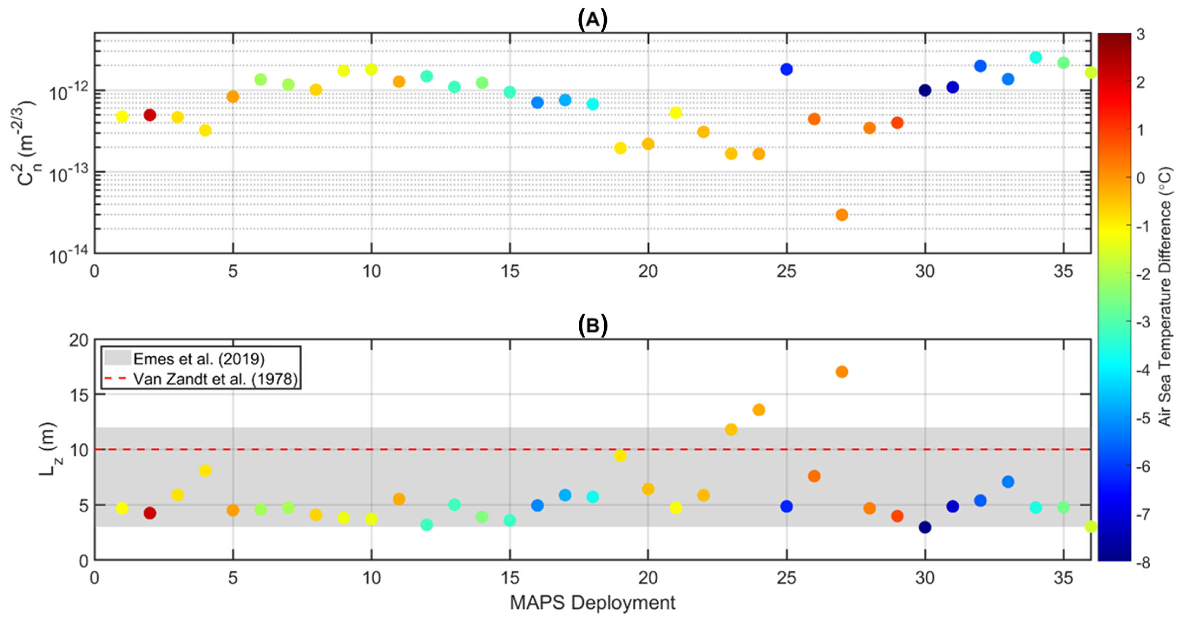
5.1. Vertical Length Scale—$L_z$

Vertical outer length scales from the PSO experiments range from 2.96 m to 17.02 m, with an average of 5.80 m over the MAPS datasets (Table 1). Bulk $C_n^2$ and corresponding $L_z$ for the 36 optimizations are illustrated in Figure 5. $L_z$ are visually compared with vertical outer length scales from [26,35] in Figure 5B. The authors of [26] estimate $L_z$ over multiple stability regimes (i.e., unstable, neutral, and stable), yielding a range of values shown as the grey shaded region in Figure 5B. These vertical length scales included from [26] are approximated at 12 m, chosen to be consistent with the TRIF model utilizing $C_n^2$ estimated from meteorological data at this altitude. Generally, $L_z$ fall close to the values reported by [26] apart from 2 MAPS datasets (24 and 27) associated with near-thermal neutrality. Because the optimized $L_z$ are generally consistent with the ranges in the literature, one can conclude that the MAPS data cloud could be largely driven by turbulence. If the optimization revealed an unrealistic/non-physical $L_z$ (e.g., at maximum/minimum value in the search space) to match the MAPS data, then that would have indicated that uncertainty could be a significant factor. Thus, MAPS-measured refractivity variance is potentially representative of physically relevant fluctuations of the refractive index.

To further confirm the physical nature of the optimized $L_z$, the correlation between $C_n^2$ and $L_z$ was examined. $L_z$ reveals a significant inverse relationship with $C_n^2$ shown by a correlation coefficient (R) of −0.53 with a p-value of <0.05. This result is contrary to expectations as it suggests decreasing vertical outer length scales as $C_n^2$ increases. Presumably, in thermally unstable conditions, the increase in buoyant effects generating convective plumes would increase both the magnitude of turbulence ($C_n^2$) and $L_z$, leading to a direct relationship. While in stable conditions, one would assume that the stable stratification would inhibit development of large-scale fluctuations.

To further investigate the indirect relationship between $C_n^2$ and $L_z$, we explored the possible sources of error in the comparisons. One source of uncertainty is due to the $C_n^2$ estimate being based on an average condition (i.e., based on bulk meteorological measurements), while the MAPS measurements used for the optimization are individually instantaneous (to order 1 s). Secondly, the assumption of a constant $C_n^2$ with altitude can also result in uncertainty. Finally, Ref. [28] reported that for ASTD > −1 °C, bulk $C_n^2$ estimates deviate from scintillation-derived (SD) $C_n^2$. For cases of near-thermal neutrality (−0.5 °C < ASTD < 0.5 °C), bulk $C_n^2$ can underestimate SD $C_n^2$ by more than 1 order of magnitude for certain wind and humidity conditions. This underestimation can presumably explain MAPS deployment 27, where near-neutral conditions were observed (ASTD = 0.11 °C) corresponding to an abnormally low $C_n^2$ (2.97 × 10⁻¹⁴ m^−2/3) and the largest $L_z$ (17.02 m). This underestimation of $C_n^2$ effectively leads to overestimation of $L_z$ to match the observed fluctuations; MAPS dataset 24 is similar, where a near-neutral environment was also observed (ASTD = −0.26 °C). For these cases, the relatively small $C_n^2$ does not correspond with relatively small RMS MAPS refractive fluctuations, and thus a large $L_z$ is derived by the optimization compensating for the small $C_n^2$. Further, Ref. [28] also reported that during periods of thermal stability (ASTD > 1 °C), bulk $C_n^2$ estimates can be overestimated by up to 1 order of magnitude. For this study, the overestimation of $C_n^2$ would lead to derived $L_z$ that are smaller than expected. These uncertainties in NAVSLaM bulk $C_n^2$ estimates could cause the indirect relationship between $C_n^2$ and $L_z$. Thus, since $L_z$ fall within the previously reported ranges of vertical outer length scales and considering some stability-dependent error in the bulk estimation of $C_n^2$, it is plausible that the majority of the refractive fluctuations in the MAPS measurements are indicative of inertial to large-scale turbulent physical processes.

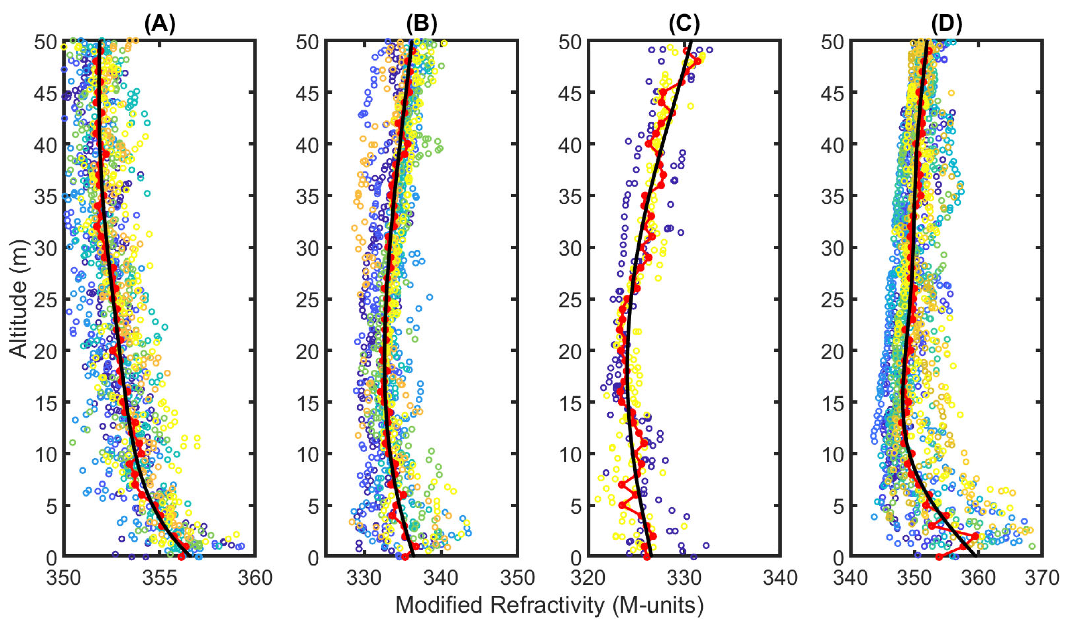
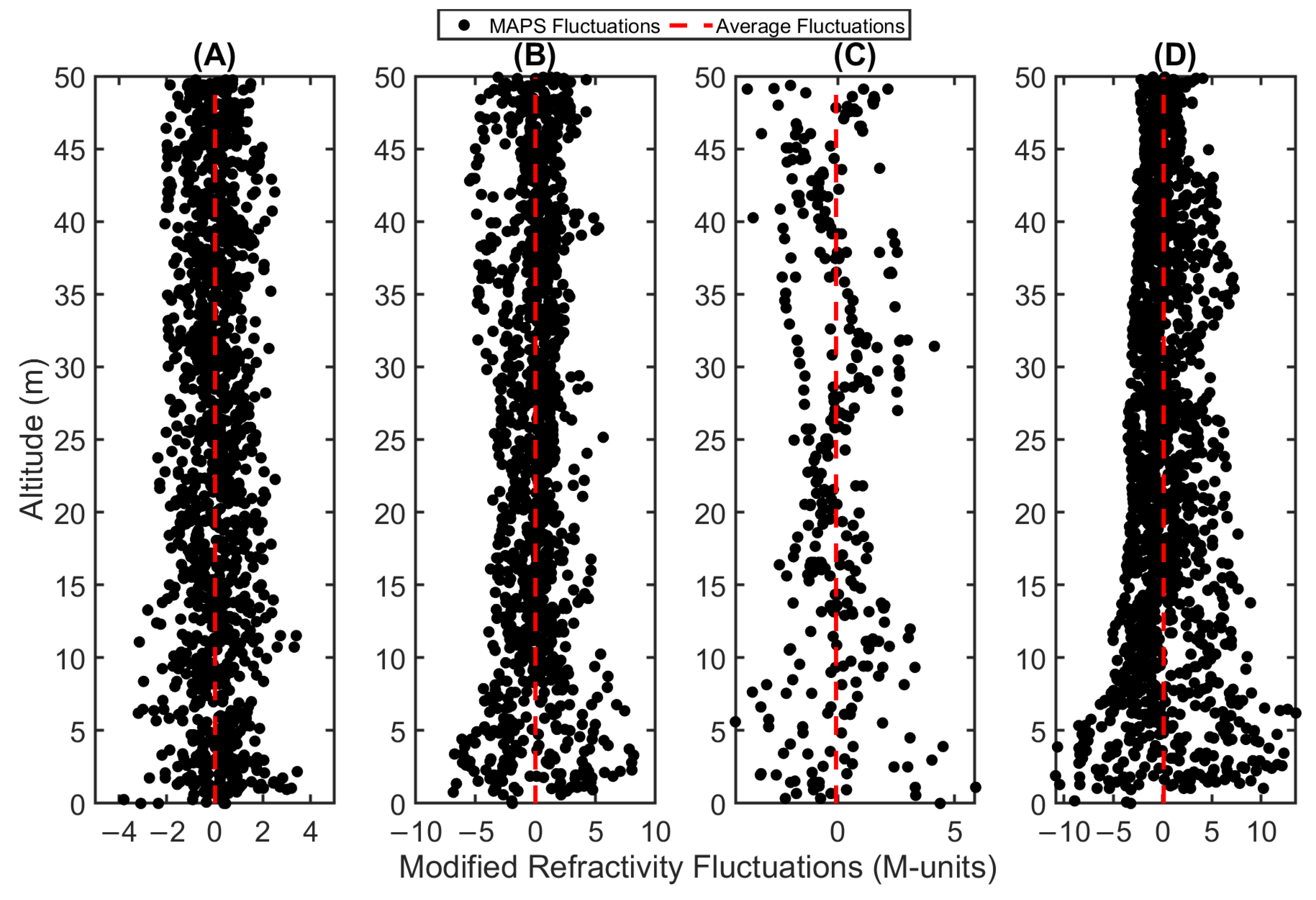
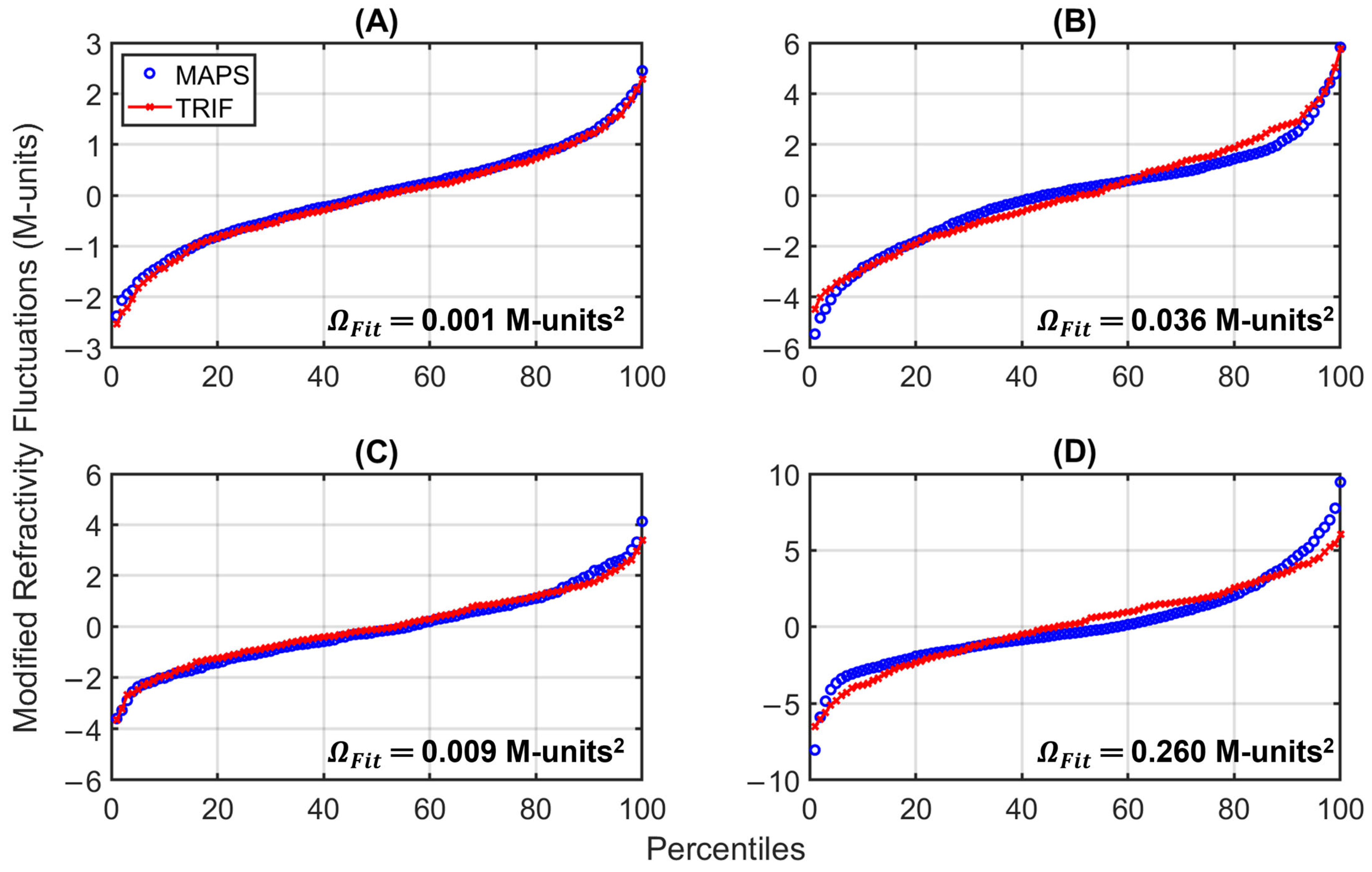
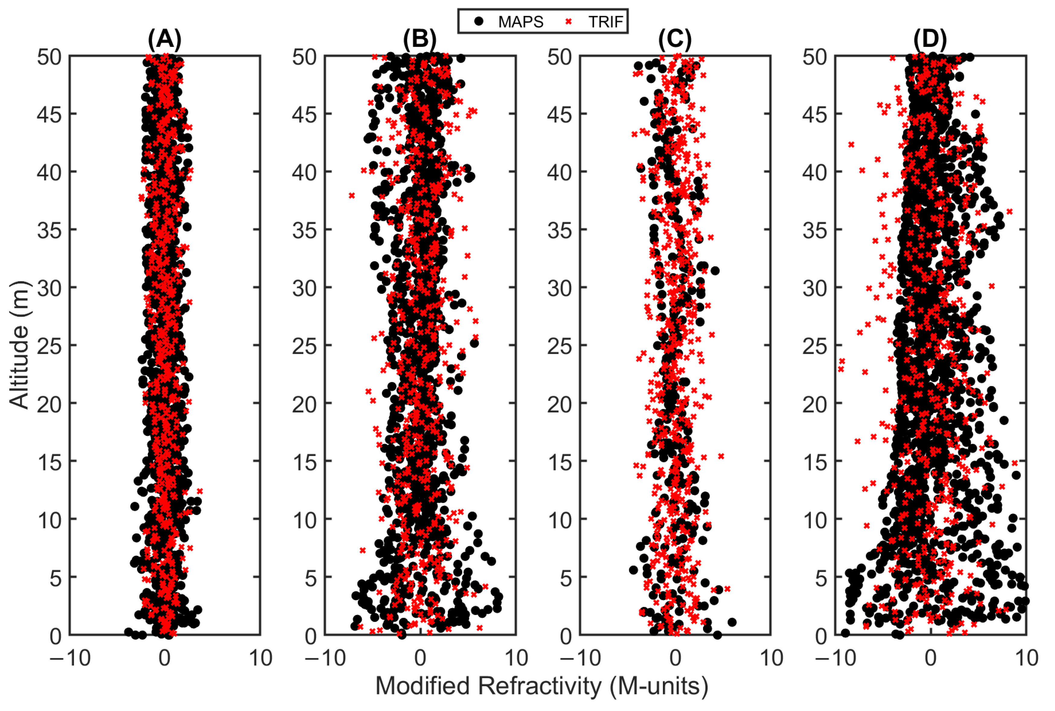
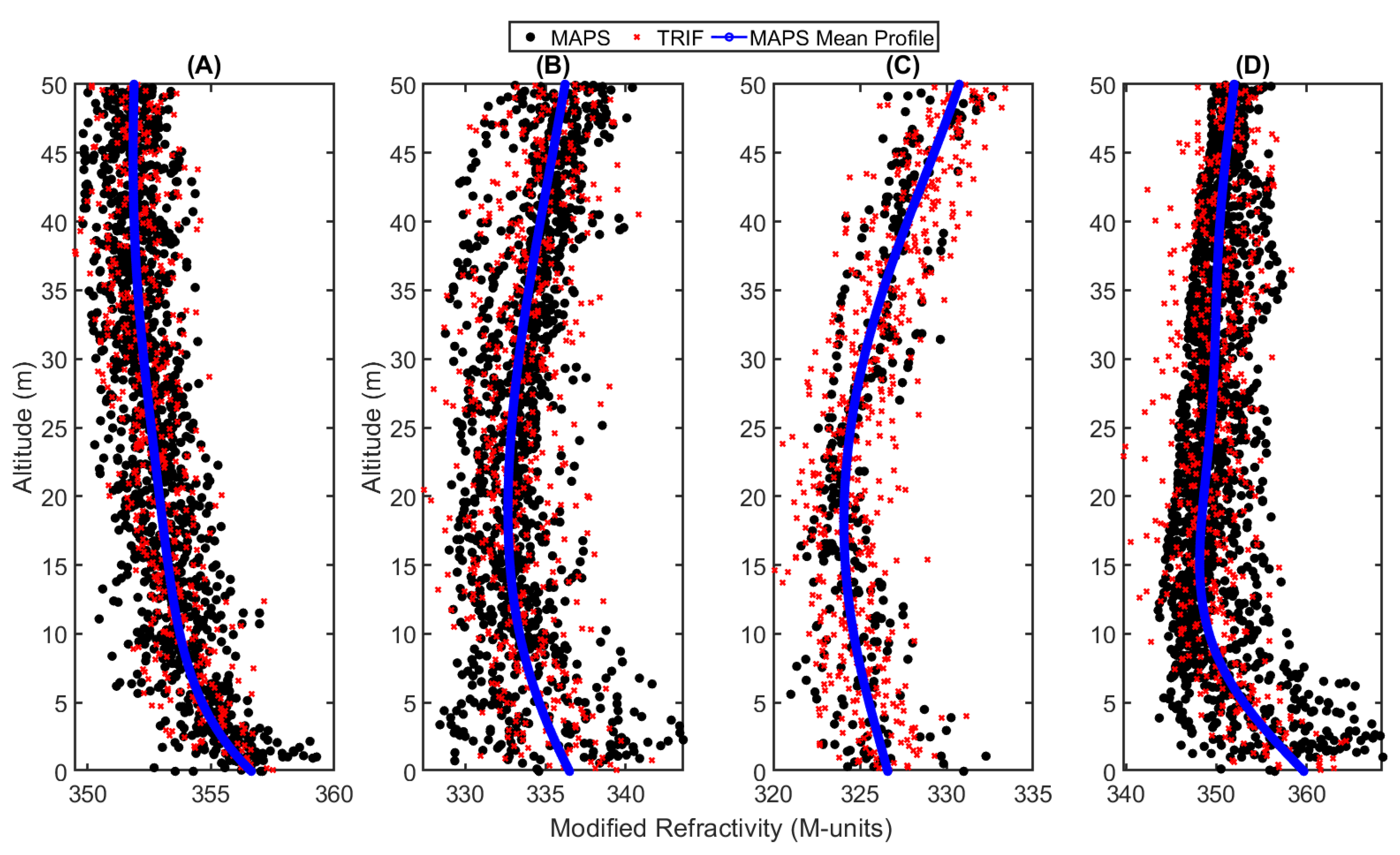
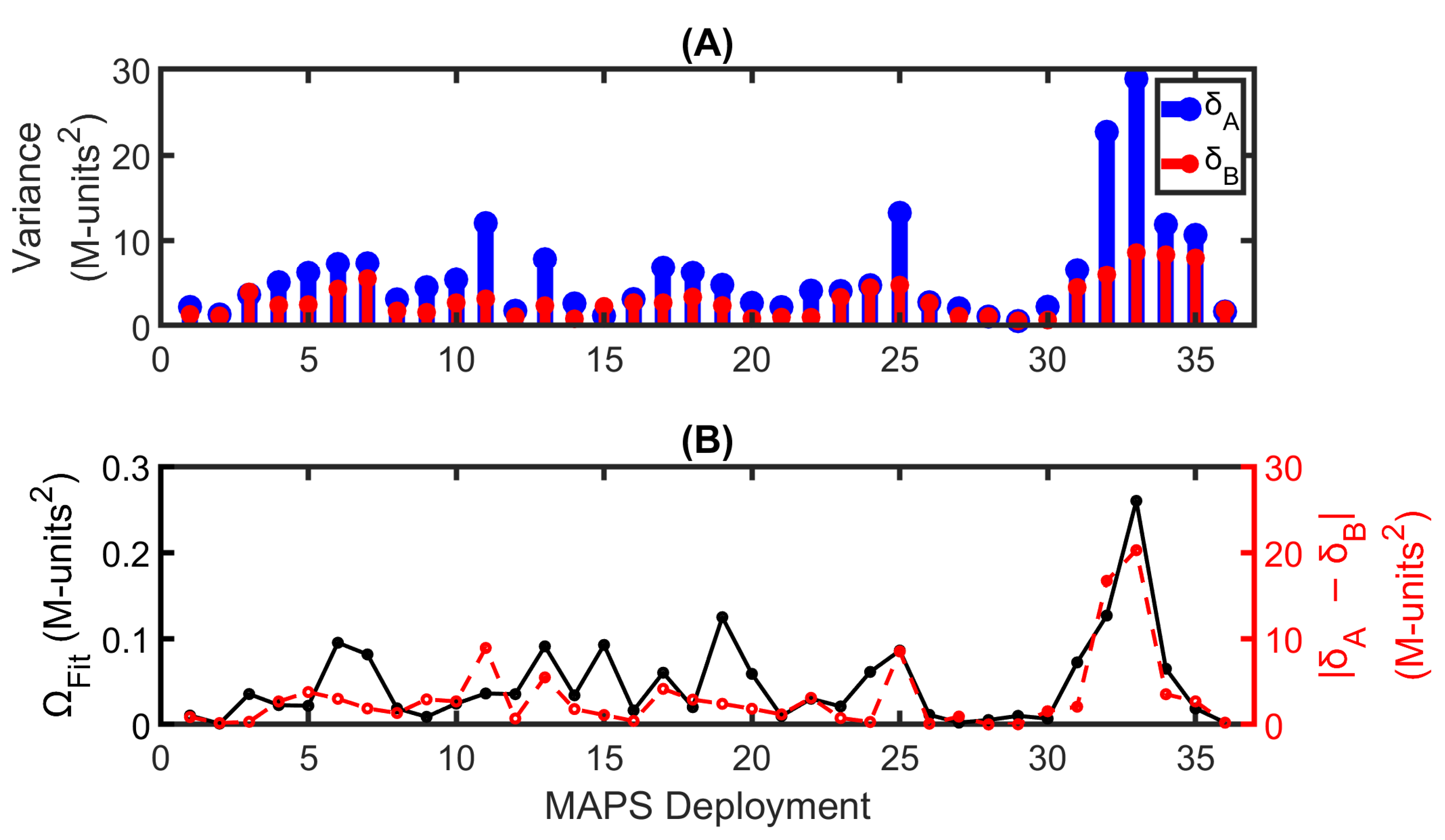
5.2. Refractive Fluctuations

TRIF-modeled refractivity fluctuations using $L_z$ derived via PSO for the example MAPS datasets (2, 11, 9, and 33) are illustrated in Figure 6, and the associated instantaneous distributions of refractivity are displayed in Figure 7. For these examples, TRIF model fluctuations optimized to corresponding MAPS refractivity have a ${\mathsf{\Omega }}_{Fit}$ of 0.001 M-units² (Figure 6A), 0.036 M-units² (Figure 6B), 0.009 M-units² (Figure 6C), and 0.260 M-units² (Figure 6D), for MAPS datasets 2, 11, 9, and 33, respectively. The discrepancies between the ${\mathsf{\Omega }}_{Fit}$ for the examples displayed in Figure 6 are visually apparent. TRIF fluctuations mostly occur within the bounds of MAPS refractivity in Figure 6A–C, corresponding to relatively low ${\mathsf{\Omega }}_{Fit}$; this is not the case for Figure 6D. Most datasets (32 of 36) are on the order of the mean ${\mathsf{\Omega }}_{Fit}$ (0.047 M-units²) and are visually akin to Figure 6B. In Figure 6D, TRIF fluctuations tend to have a greater magnitude than MAPS refractivity at altitudes greater than ~8 m and fail to span MAPS fluctuations below this 8 m altitude. Consequently, MAPS dataset 33 corresponds to the largest (worst) ${\mathsf{\Omega }}_{Fit}$ relative to all MAPS deployments. This vertical inhomogeniety is not accounted for in the TRIF model as turbulence is assumed homogenous with altitude—i.e., $C_n^2$ and $L_z$ are estimated as one value for the entire profile.

The assumption of homogenous turbulence within TRIF is questionable for $C_n^2$ in the surface layer [18,21,36,37] but is a reasonable assumption for $L_z$ [18]. Thus, the assumption of $C_n^2$ homogeneity is presumably a main driver of variation in fitness scores over the 36 datasets. The altitudinal inhomogeneity is illustrated in Figure 8, where fitness score is shown relative to altitudinal variance in the MAPS data. $M^{\prime }$ variance was computed over 2 altitudinal bins, 0–10 m (${\delta }_A$) and 10–20 m (${\delta }_B$), exploring the vertical heterogeneity of the refractivity. ${\delta }_A$ is larger than ${\delta }_B$ for 28 of the 36 datasets, showing that the assumption of vertical homogeneity is not ideal (Figure 8A). Additionally, this result gives physical context to variations in the MAPS measurements, further supporting the physical nature of the MAPS-measured fluctuations, as one would expect turbulent fluctuation magnitudes to be largest near the surface.

Generally, the datasets shown to have the largest differences between ${\delta }_A$ and ${\delta }_B$ correspond to the largest fitness scores (poorest fit between MAPS and TRIF refractive fluctuations). This result (Figure 8B) was verified through linear correlation between ${\mathsf{\Omega }}_{Fit}$ and $\left|{\delta }_A-{\delta }_B\right|$, yielding $R=$ 0.75 ($p$ < 0.05), a significant direct relationship. Thus, as the assumption of vertically homogenous turbulence degrades, so follows the TRIF model accuracy; however, even the largest $\sqrt{{\mathsf{\Omega }}_{Fit}}$ are small relative to the RMS $M^{\prime }$ (Table 1), suggesting that TRIF can adequately model fluctuations in the cases presented. This result further suggests that PSO-estimated $L_z$ falling within the ranges presented in Figure 5 are plausible and support the notion that MAPS variances are primarily related to physical processes.

6. Summary and Conclusions

This study incorporated unique meteorological data acquired with MAPS, deployed during the CASPER-East field campaign [11]. These data were used to examine the physical significance of variability within those measurements, performed within the MASL. MAPS [9] is a cutting edge MASL measurement technique able to obtain vertical distributions of pressure, temperature, humidity, and, thus, refractivity at relatively high temporal resolution. The goal of this study was to investigate the variance captured by these MAPS measurements and determine whether it can be explained by turbulent physical processes. To do this, the turbulence refractive index fluctuation (TRIF) model was implemented. TRIF is a spectral turbulence model based on a 1-D vertically homogenous anisotropic Kolmogorov spectrum that includes parameters describing the magnitude of the refractive index fluctuations ($C_n^2$) and vertical turbulent outer length scale ($L_z$). $C_n^2$ was estimated via bulk methods from MAPS and R/V Sharp meteorological measurements including SST, implemented via NAVSLaM. $L_z$ was derived via PSO utilizing TRIF for 36 MAPS datasets of modified refractivity, which were decomposed into fluctuations. The derived $L_z$ were compared with previously reported values in the MASL, and the accuracy of TRIF to properly emulate MAPS fluctuations was evaluated.

Optimized solutions of $L_z$ are generally in good agreement with previously reported values in the MASL [26], where 94% of $L_z$ solutions fall within a range observed in [26] over a wide range of atmsopheric stability conditions. Two $L_z$ are greater than the reported range, where these $L_z$ occur during near-thermally neutral conditions, likely causing underestimation of bulk $C_n^2$ (resulting in the large $L_z$), as previously reported [28]. Furthermore, for periods of thermal stability, NAVSLaM has been shown to overestimate bulk $C_n^2$, contributing to possible underestimation in the derived $L_z$. These uncertainties in $C_n^2$ can at least partly explain why the $L_z$ estimates are within the correct order of magnitude but may not follow expected trends with air–sea temperature difference (ASTD).

Fluctuations from the TRIF model, based on optimization to MAPS measurements, were further examined by highlighting the relationship between fitness scores (${\mathsf{\Omega }}_{Fit})$ and variations in MAPS fluctuations as a function of altitude. Specifically, when the assumption of $C_n^2$ homogeneity degrades, ${\mathsf{\Omega }}_{Fit}$ increase. Vertical heterogeneity was observed, to some degree, for all MAPS datasets, further suggesting the physical nature of the MAPS measurements’ variability. Even in cases where vertical heterogeneity is more prominent, and ${\mathsf{\Omega }}_{Fit}$ are relatively large, TRIF refractive fluctuations are generally in good agreement with the MAPS refractivity fluctuations. This result illuminates the effectiveness of the TRIF model to emulate refractive fluctuations over a variety of conditions. Thus, the authors suggest that the variability observed in MAPS-measured instantaneous refractivity is physically significant and not primarily influenced by measurement uncertainty. Future research should incorporate turbulent refractive index fluctuation models that account for vertically heterogenous $C_n^2$.

References

1. Businger, J.A.; Wyngaard, J.C.; Izumi, Y.; Bradley, E.F. Flux-profile relationships in the atmospheric surface layer. J. Atmos. Sci. 1971, 28, 181–189. [Google Scholar] [CrossRef]
2. Dyer, A.J. A review of flux-profile relationships. Bound.-Layer Meteorol. 1974, 7, 363–372. [Google Scholar] [CrossRef]
3. Webster, P.J.; Lukas, R. TOGA COARE: The coupled ocean–atmosphere response experiment. Bull. Am. Meteorol. Soc. 1992, 73, 1377–1416. [Google Scholar] [CrossRef]
4. Fairall, C.W.; Bradley, E.F.; Rogers, D.P.; Edson, J.B.; Young, G.S. Bulk parameterization of air-sea fluxes for tropical ocean-global atmosphere coupled-ocean atmosphere response experiment. J. Geophys. Res. Ocean. 1996, 101, 3747–3764. [Google Scholar] [CrossRef] [Green Version]
5. Fairall, C.W.; Bradley, E.F.; Hare, J.E.; Grachev, A.A.; Edson, J.B. Bulk parameterization of air–sea fluxes: Updates and verification for the COARE algorithm. J. Clim. 2003, 16, 571–591. [Google Scholar] [CrossRef]
6. Frederickson, P. Navy Atmospheric Measurements for EM Propagation Modeling. Executive Summary, Calhoun.nps.edu. 2016. Available online: https://www.nps.edu/en/web/research/summaries (accessed on 27 April 2023).
7. Hogan, T.; Liu, M.; Ridout, J.; Peng, M.; Whitcomb, T.; Ruston, B.; Reynolds, C.; Eckermann, S.; Moskaitis, J.; Baker, N.; et al. The navy global environmental model. Oceanography 2014, 27, 116–125. [Google Scholar] [CrossRef]
8. Grachev, A.A.; Andreas, E.L.; Fairall, C.W.; Guest, P.S.; Persson, P.O.G. SHEBA flux–profile relationships in the stable atmospheric boundary layer. Bound.-Layer Meteorol. 2007, 124, 315–333. [Google Scholar] [CrossRef]
9. Yang, Z.; Calderer, A.; He, S.; Sotiropoulos, F.; Doyle, J.D.; Flagg, D.D.; MacMahan, J.; Wang, Q.; Haus, B.K.; Graber, H.C.; et al. Numerical Study on the Effect of Air–Sea–Land Interaction on the Atmospheric Boundary Layer in Coastal Area. Atmosphere 2018, 9, 51. [Google Scholar] [CrossRef] [Green Version]
10. Doreene, K.; Wang, Q. Optimized estimation of surface layer characteristics from profiling measurements. Atmosphere 2016, 7, 14. [Google Scholar]
11. Wang, Q.; Alappattu, D.P.; Billingsley, S.; Blomquist, B.; Burkholder, R.J.; Christman, A.J.; Creegan, E.D.; De Paolo, T.; Eleuterio, D.P.; Fernando, H.J.S.; et al. CASPER: Coupled air–sea processes and electromagnetic ducting research. Bull. Am. Meteorol. Soc. 2018, 99, 1449–1471. [Google Scholar] [CrossRef]
12. Wang, Q.; Franklin, K.; Yamaguchi, R.; Ortiz-Suslow, D.G.; Alappattu, D.P.; Yardim, C.; Burkholder, R. Ducting conditions during casper-west field campaign. In Proceedings of the 2018 IEEE International Symposium on Antennas and Propagation & USNC/URSI National Radio Science Meeting, Boston, MA, USA, 8–13 July 2018; pp. 877–878. [Google Scholar]
13. Rainer, R.B. In-Situ Observation of Undisturbed Surface Layer Scaler Profiles for Characterizing Evaporative Duct Properties; Naval Postgraduate School Monterey United States: Monterey, CA, USA, 2016. [Google Scholar]
14. Alappattu, D.P.; Wang, Q.; Rainer, R.; Yamaguchi, R.; Lind, R.J. 4.4 Characteristics of surface layer scalar profiles using the in-situ measurements from an undisturbed marine environment. In Proceedings of the 20th Conference on Air–Sea Interaction, Madison, WI, USA, 15–19 August 2016; American Meteorological Society: Boston, UK, 2016. [Google Scholar]
15. Ulate, M.; Wang, Q.; Haack, T.; Holt, T.; Alappattu, D.P. Mean offshore refractive conditions during the CASPER East field campaign. J. Appl. Meteorol. Climatol. 2019, 58, 853–874. [Google Scholar] [CrossRef]
16. Pastore, D.M.; Greenway, D.P.; Stanek, M.J.; Wessinger, S.E.; Haack, T.; Wang, Q.; Hackett, E.E. Comparison of atmospheric refractivity estimation methods and their influence on radar propagation predictions. Radio Sci. 2021, 56, 1–17. [Google Scholar] [CrossRef]
17. Pastore, D.M.; Wessinger, S.E.; Greenway, D.P.; Stanek, M.J.; Burkholder, R.J.; Haack, T.; Wang, Q.; Hackett, E.E. Refractivity inversions from point-to-point X-band radar propagation measurements. Radio Sci. 2022, 57, 1–16. [Google Scholar] [CrossRef]
18. Rouseff, D. Simulated microwave propagation through tropospheric turbulence. IEEE Trans. Antennas Propag. 1992, 40, 1076–1083. [Google Scholar] [CrossRef]
19. Ivanov, V.K.; VShalyapin, N.; Levadny, Y.V. Microwave scattering by tropospheric fluctuations in an evaporation duct. Radiophys. Quantum Electron. 2009, 52, 277–286. [Google Scholar] [CrossRef]
20. Levadnyi, I.; Ivanov, V.; Shalyapin, V. Simulation of microwave propagation in turbulent evaporation duct. In Proceedings of the 2012 6th European Conference on Antennas and Propagation (EUCAP), Prague, Czech Republic, 26–30 March 2012; IEEE: Piscataway, NJ, USA, 2012; pp. 1–3. [Google Scholar]
21. Chou, Y.-H.; Kiang, J.-F. Effect of turbulence on wave propagation in evaporation ducts above a rough sea surface. In Forum for Electromagnetic Research Methods and Application Technologies; University of Limoges: Limoges, France, 2014; Volume 12. [Google Scholar]
22. Wagner, M.; Gerstoft, P.; Rogers, T. Estimating refractivity from propagation loss in turbulent media. Radio Sci. 2016, 51, 1876–1894. [Google Scholar] [CrossRef] [Green Version]
23. Bean, B.R.; Dutton, E.J. Radio Meteorology; Superintendentof Documents; U.S. Government Publishing Office: Washington, DC, USA, 1966; Volume 92.
24. Buck, A.L. New equations for computing vapor pressure and enhancement factor. J. Appl. Meteorol. Climatol. 1981, 20, 1527–1532. [Google Scholar] [CrossRef]
25. Ishimaru, A. Wave Propagation and Scattering in Random Media; Academic Press: New York, NY, USA, 1978; Volume 2. [Google Scholar]
26. Emes, M.J.; Arjomandi, M.; Kelso, R.M.; Ghanadi, F. Turbulence length scales in a low-roughness near-neutral atmospheric surface layer. J. Turbul. 2019, 20, 545–562. [Google Scholar] [CrossRef]
27. Percival, D.B. Simulating Gaussian random processes with specified spectra. Comput. Sci. Stat. 1993, 24, 534. [Google Scholar]
28. Frederickson, P.A.; Davidson, K.L.; Zeisse, C.R.; Bendall, C.S. Estimating the refractive index structure parameter () over the ocean using bulk methods. J. Appl. Meteorol. 2000, 39, 1770–1783. [Google Scholar] [CrossRef]
29. Frederickson, P.A.; Hammel, S.; Tsintikidis, D. Improving bulk Cn2 models for over-ocean applications through new determinations of the dimensionless temperature structure parameter. In Atmospheric Optics: Models, Measurements, and Target-in-the-Loop Propagation; SPIE: Bellingham, WA, USA, 2007; Volume 6708, pp. 45–54. [Google Scholar]
30. Qing, C.; Wu, X.; Li, X.; Tian, Q.; Liu, D.; Rao, R.; Zhu, W. Simulating the refractive index structure constant in the surface layer at Antarctica with a mesoscale model. Astron. J. 2017, 155, 37. [Google Scholar] [CrossRef] [Green Version]
31. Kennedy, J.; Eberhart, R. Particle swarm optimization. In Proceedings of the ICNN’95-International Conference on Neural Networks, Perth, WA, Australia, 27 November–1 December 1995; IEEE: Piscataway, NJ, USA, 1995; Volume 4, pp. 1942–1948. [Google Scholar]
32. Poli, R.; Kennedy, J.; Blackwell, T. Particle swarm optimization. Swarm Intell. 2007, 1, 33–57. [Google Scholar] [CrossRef]
33. Tatarskii, V.I. The Effects of the Turbulent Atmosphere on Wave Propagation; Israel Program for Scientific Translations: Jerusalem, Israel, 1971. [Google Scholar]
34. Wheelon, A.D. Electromagnetic Scintillation: Volume 1, Geometrical Optics; Cambridge University Press: Cambridge, UK, 2001. [Google Scholar]
35. VanZandt, T.E.; Green, J.L.; Gage, K.S.; Clark, W.L. Vertical profiles of refractivity turbulence structure constant: Comparison of observations by the Sunset radar with a new theoretical model. Radio Sci. 1978, 13, 819–829. [Google Scholar] [CrossRef]
36. Panofsky, H.A. Atmospheric turbulence. In Models and Methods for Engineering Applications; Wiley: New York, NY, USA, 1984; Volume 397. [Google Scholar]
37. Geernaert, G.L. Surface layer. In Encyclopedia of Atmospheric Sciences; Elsevier: Amsterdam, The Netherlands, 2003; pp. 305–311. [Google Scholar]
Figure 1. Time series of meteorological variables measured aboard the R/V Sharp and based-on the 7th-order polynomial fit of the MAPS data. (A) Shows wind speed and specific humidity and (B) shows air temperature, sea-surface temperature, and air pressure (see legends). All meteorological parameters were measured at an altitude of 12 m above mean sea level and are displayed for all MAPS deployment times during the CASPER-East field campaign (Table 1).
Atmosphere 14 01085 g001
Figure 2. Example MAPS datasets corresponding to datasets 2 (A), 11 (B), 9 (C), and 33 (D) (Table 1). Circles represent the modified refractivity computed via (1) from the instantaneous measurements obtained from MAPS, where the black line is the 7th-order polynomial fit representing the mean refractivity profile, and the red line represents a 1 m bin-averaged profile. Colors included for the instantaneous refractivity measurements correspond to different launches (single ascent and descent) of MAPS.
Atmosphere 14 01085 g002
Figure 3. Fluctuations ( M z ) computed via (2) corresponding to the MAPS datasets in Figure 2 (A) (dataset) 2, (B) 11, (C) 9, (D) 33. The red dashed line shows the mean of the fluctuations verifying the 7th-order polynomial fit as a good measure of the mean.
Atmosphere 14 01085 g003
Figure 4. Quantiles for the example MAPS fluctuations illustrated in Figure 3, and quantiles for the associated TRIF model fluctuation predictions realized via particle swarm optimization of L z . An array of optimization results are displayed in this figure: the dataset with (A) the lowest fitness score (dataset 2), (B) the fitness score nearest to the mean over all optimizations (dataset 11), (C) the MAPS dataset with the fewest measurements (dataset 9), and (D) the largest fitness score (dataset 33). Fitness scores ( Ω F i t ) for each example are included in each panel.
Atmosphere 14 01085 g004
Figure 5. (A) Refractive index structure constant ( C n 2 ) estimated via NAVSLaM from the environmental variables displayed in Figure 1 for each MAPS deployment. (B) L z solutions from the particle swarm optimization corresponding to each MAPS dataset. Included in (B) are previously reported ranges of L z in the atmospheric surface layer (at ~12 m above the boundary) from [26] for differing atmospheric stability regimes (gray shaded region) and L z reported in [35] for the free atmosphere (10 m) (red dashed line). Marker colors denote the air–sea temperature difference in both panels.
Atmosphere 14 01085 g005
Figure 6. Refractive index fluctuations corresponding to example MAPS datasets in Figure 1, Figure 2, Figure 3 and Figure 4 along with TRIF model fluctuations using the particle swarm optimization-based vertical outer turbulent length scale. ((A) (dataset) 2, (B) 11, (C) 9, (D) 33).
Atmosphere 14 01085 g006
Figure 7. MAPS and TRIF instantaneous refractivity and the corresponding MAPS 7th-order polynomial fit for the MAPS datasets previously described in Figure 2, Figure 3, Figure 4 and Figure 6 ((A) (dataset) 2, (B) 11, (C) 9, (D) 33).
Atmosphere 14 01085 g007
Figure 8. (A) Altitudinal variance in MAPS refractive fluctuations ( M ). M variance displayed for altitudes spanning 0–10 m and 10–20 m, δ A and δ B , respectively. (B) The left axis illustrates fitness scores (Equation (10)) corresponding to the MAPS/TRIF optimizations for each dataset in black, shown in Table 1. The magnitude of difference in MAPS refractive fluctuation variance between the 0–10 m and 10–20 m altitudinal bins ( δ A δ B ) is illustrated in red on the right-hand axis.
Atmosphere 14 01085 g008