1. Introduction
Despite the widespread and growing impact of emissions on our health and environment, there remains an unmet need for emission concentration models. Anthropogenic activity is the greatest contributor to these emissions, with the most significant sources being point sources such as power plants and manufacturing factories, contributing 31% and 12%, respectively [
1,
2]. As a consequence, every year, more than seven million people die prematurely due to air pollution [
3], with one in five people dying of air pollution from greenhouse gas emissions [
4]. Yet despite the mounting consequences, our emissions continue to grow, as noted in the latest report from the Intergovernmental Panel on Climate Change [
5]. This growth in emissions, combined with mounting global warming concerns, makes addressing emissions increasingly important. It is imperative that we take informed and strategic action using tools such as emission models to curb our greenhouse gas emissions before it is too late.
Conventional emission models represent the spatial and temporal variation of substances such as greenhouse gases (GHGs) emitted at the emission source or after release [
1]. At the source, an accounting of total emissions is carried out to conduct emission inventories. The emission inventory consists of data reported by emitters in accordance with regulations using prescribed, sector-specific calculation methods such as the emission factor, which relates the quantity of emissions from a source to units of activity associated with emission release. However, these factors are typically averages of available data and result in emission inventories that are primarily useful as a knowingly gross estimation of emission trends [
6,
7]. After release, air dispersion models such as Gaussian plume models like the AMS/EPA Regulatory Model (AERMOD [
8]) and the California Air Resources Board’s puff model (CALPUFF [
9]) are used to simulate the mixture of an emission with the atmosphere. These models characterize key processes that control dispersion and may be used to predict the concentration further in space and time. However, these models are limited by their lack of generalizability and by the significant computational time and resources required [
10,
11].
This work aims to address the research gap in emission concentration modeling by proposing a novel approach using quantum machine learning for the spatiotemporal prediction of emission concentrations. While conventional models have limitations in their generalizability and computational resources required, our quantum machine learning approach shows promise with improvements in accuracy and efficiency. This paper explores the effectiveness of our quantum machine learning approach by developing a quantum quanvolutional neural network model and comparing it to a classical spatiotemporal ConvLSTM model using an evaluation framework of baseline models and metrics of per-pixel loss and intersection over union accuracy.
2. Materials and Methods
This work focuses on formulating emission concentration modelling as a quantum machine learning problem and setting up a foundation upon which increasingly complex models can be built. To achieve this, six steps were taken, each building upon the previous one to create a comprehensive evaluation framework. Firstly, the problem scope was narrowed to focus on one-hour-ahead emission concentration forecasting. Secondly, data used to develop the models were prepared. Thirdly, baseline models were created to provide a basis for comparison with the developed models. These models were random and input-independent models which served as a benchmark for evaluating the performance of the more complex models. Fourthly, metrics for accuracy and loss were developed to evaluate the performance of the models. These included metrics of per-pixel loss and an intersection over union accuracy. These metrics were used to compare the classical, quantum, and baseline models. Fifthly, a simple classical ConvLSTM model was developed to demonstrate usage of the evaluation framework. Sixthly, a quantum quanvolutional neural network model was developed. The resultant classical, quantum, and baseline models were then compared using the metrics developed.
2.1. Problem Scope
The problem of forecasting emission concentration from point sources, as shown above in
Figure 1, was chosen due to the ease of data collection and the fact that point sources account for 70% of all emissions [
5].
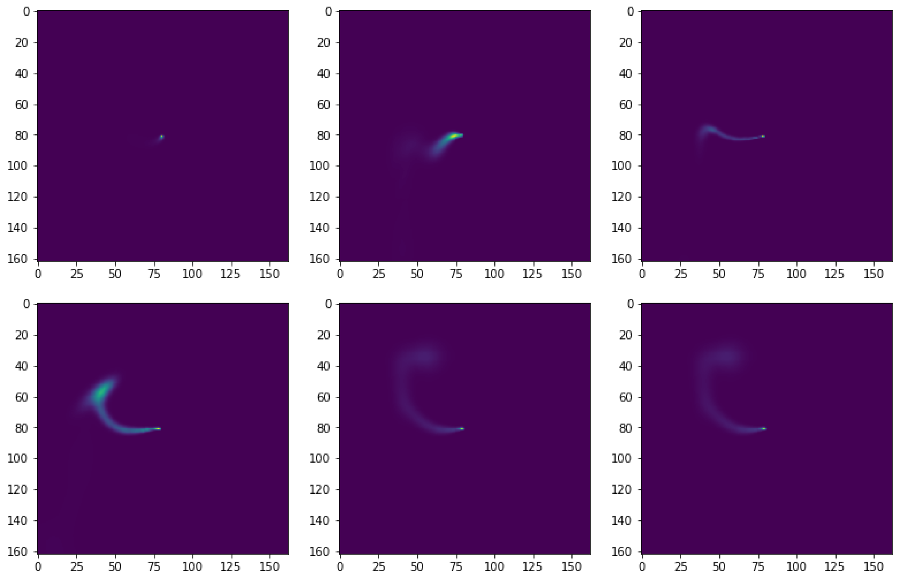
The toy problem chosen for the developed models was to generate one-hour-ahead predictions of emission concentration, given an input sequence of the past six-hour emission concentrations from the same point source. The forecast would be made assuming no significant change in land use or buildings.
2.2. Data
Training data were provided by Lakes Environmental Research and included spatiotemporal concentration data from various point sources. Concentrations were measured 10 m above the ground within a square geofenced region around various point sources. Concentration values were normalized and centred within a 162 × 162 matrix. Each dataset contained 35,040 data points, with one data point every 15 min generated over one year. All data were shuffled and then split 80:20 using the Pareto principle into the data used to train the models (the training dataset) and the data used to evaluate the fit of the final model (the test dataset). The training dataset was then split 80:20, with 20% reserved as the validation dataset for evaluating model fit while tuning the model hyperparameters. The training, validation, and test sets consisted of 64%, 16%, and 20% of the data, respectively.
2.3. Baselines
Baseline models were developed to generate outputs that could serve as meaningful reference points to compare the classical and quantum model predictions against. By comparing solutions to baseline outputs, the impact of changes to the models developed and changes in data fed to the models on the predictions generated could be evaluated.
Two baselines were developed: (1) a random chance benchmark and (2) an input-independent benchmark.
The random chance model was developed to represent randomly guessing the concentration and wind field. This corresponded to a model that returned a tensor filled with randomly generated values as its output prediction regardless of the input image. This output served as an accuracy baseline lower bound, as it was expected that any model created would have higher accuracy than randomly guessing.
The input-independent model was developed to predict the majority value in each dataset, regardless of the input. In the toy problem formulated above, the primary value of concentration in the data was zero (there were generally no emissions except where the plume was located). As a result, the input-independent model developed predicted a concentration of zero regardless of the input image. This served as a baseline closer to the ground truth to compare the accuracy of the models created against. Any model created was expected to have higher accuracy than the prediction of no emission plume concentration anywhere.
2.4. Metrics
Two metrics were chosen to evaluate the models against the baselines developed. These metrics were for loss and prediction accuracy.
For loss, a loss function was created that measured the difference between the pixel values of predicted and true images. Two standard metrics typically used are per-pixel loss functions using mean absolute error and mean square error. A per-pixel loss function quantifies the total of all errors between the exact pixel in each image. This is generally a mean absolute error calculation, also known as L1 loss.
Instead of mean absolute error, this work used the mean square error or L2 loss. This involved squaring the error instead of taking the absolute value because mean square error has mathematical properties, making it easier to calculate gradients and backpropagate error [
12]. The equation used for mean square error for the per-pixel loss function is shown below in Equation (
1).
, where if
y and
were identical pixel values, their difference would be 0. There are several drawbacks to using per-pixel loss functions. In summing the error of each pixel, content similarities are ignored. A more refined loss function will be created in future work that primarily captures high-level differences between image content. For example, where a per-pixel loss function would return a large error for two identical images except for being shifted by one pixel, a perceptual loss function could return a small to zero error [
13]. However, a differentiable and quickly calculated indication of accuracy was selected for this preliminary work. The per-pixel L2 loss function was chosen as a foundational metric that could later be modified to add additional terms such as perceptual loss or log-loss considering predicted probabilities.
For accuracy, an intersection over union metric was created. This metric for model accuracy measured how similar images of the predicted plumes generated by the trained models were to images of the actual plume. The first indicator that could have been used was the final per-pixel loss, as defined above, using either L1 or L2 loss. However, because the accuracy was to be evaluated on the trained models, accuracy metrics could be developed that were not differentiable and better captured high-level differences between image content.
As the accuracy in this application was human-interpretable, one measure of accuracy that could have been used was the evaluated human accuracy. Manually looking at each predicted plume image overlaid on an actual plume image could have checked how well the two images line up. However, interpretation needed to be scaled up to evaluate the accuracy of model predictions deployed on a large amount of test data. The metric chosen to capture some of this interpretation was intersection over union (IoU) shown below in Equation (
2).
, where if
y and
were identical images, their calculated IoU would be 1. To define the plume areas of intersection (∩) and union (∪) in the predicted and true images, pixel values in both images were converted to True or False based on a threshold of concentration pixel value of 0. The logical AND was taken based on thresholded pixel values for the intersection and the logical OR was taken on the thresholded pixel values for the union. The total IoU calculation for a test dataset then recorded the average IoU values across all predicted and true images.
2.5. Classical ConvLSTM
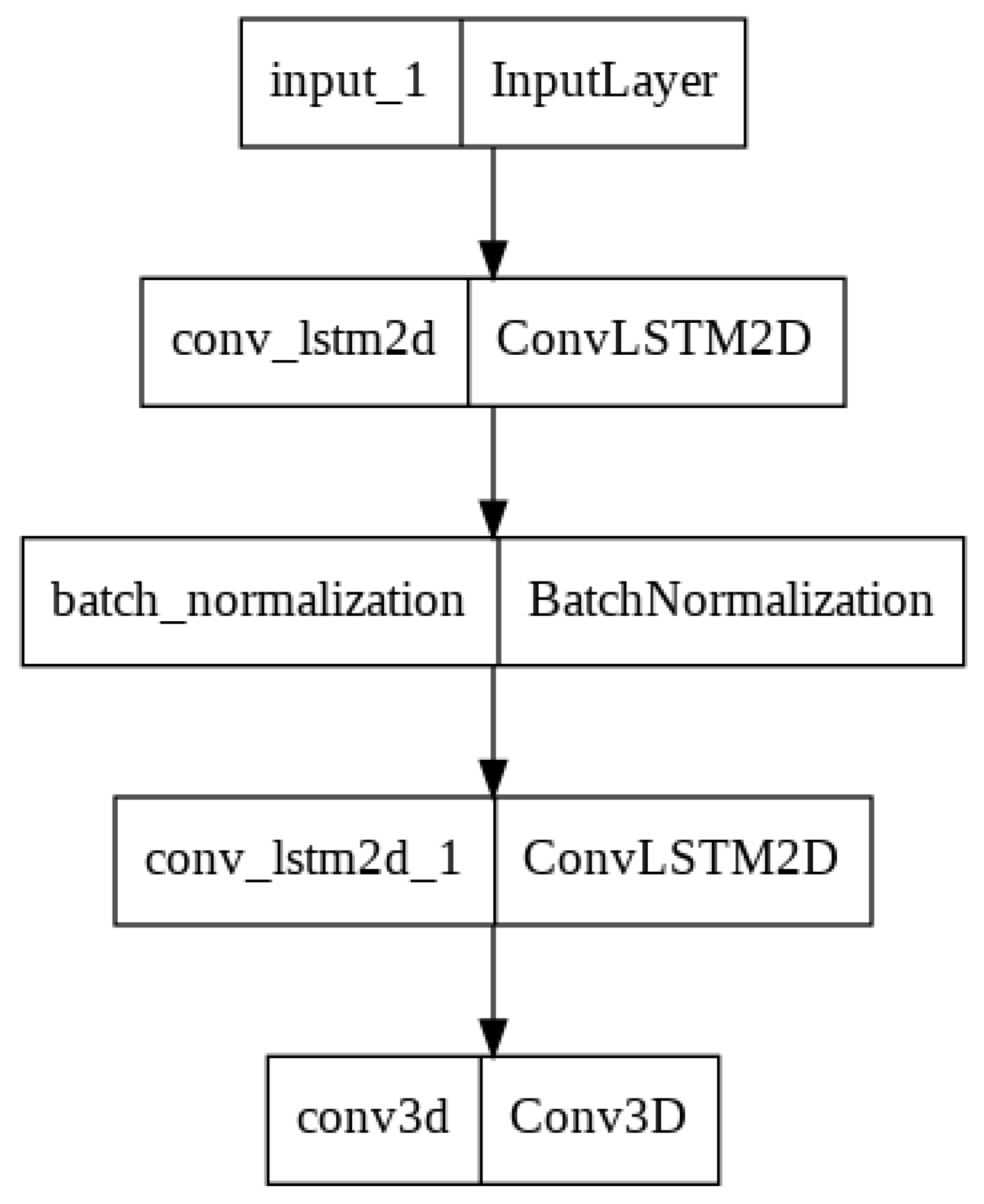
A simple classical ConvLSTM model [
14] was developed consisting of two ConvLSTM2D layers with batch normalization, followed by a Conv3D layer for the spatiotemporal outputs. The ConvLSTM network was chosen as a simple first model to check the correctness of the training and evaluation framework and as a classical counterpart to compare to the quantum model developed. The ConvLSTM developed was trained on the emission concentration dataset for the one-hour- and two-hours-ahead concentration prediction. The predictions were compared to the baseline models using the metrics.
Figure 2 shows the general architecture of the model.
2.6. Quantum-Classical Quanvolutional Neural Network
A small quanvolutional neural network [
15] was chosen as a simple quantum-classical model to check the correctness of the training and evaluation skeleton and compare it to the classical ConvLSTM model. We chose the quanvolutional neural network of Henderson et al. [
15] because it would be easy to incorporate as a single pre-processing quanvolutional layer in our hybrid quantum-classical model and because of its intended use for image analysis, which made it the easiest to test the existing training and evaluation skeleton on. Other architectures we considered included the Cong et al. QCNN [
16], the Li et al. QDCNN [
17], and the Wei et al. QCNN [
18]. The Cong et al. QCNN method was intended for learning and classifying phases of quantum physical systems not for image analysis; thus, it would not work well for our application. The Li and Wei methods were promising for future work but had drawbacks. The Li et al. QDCNN involves implementing the QRAM algorithm [
19], which would be computationally expensive. The recent Wei et al. QCNN on NISQ devices seemed promising but required more data to achieve high accuracy.
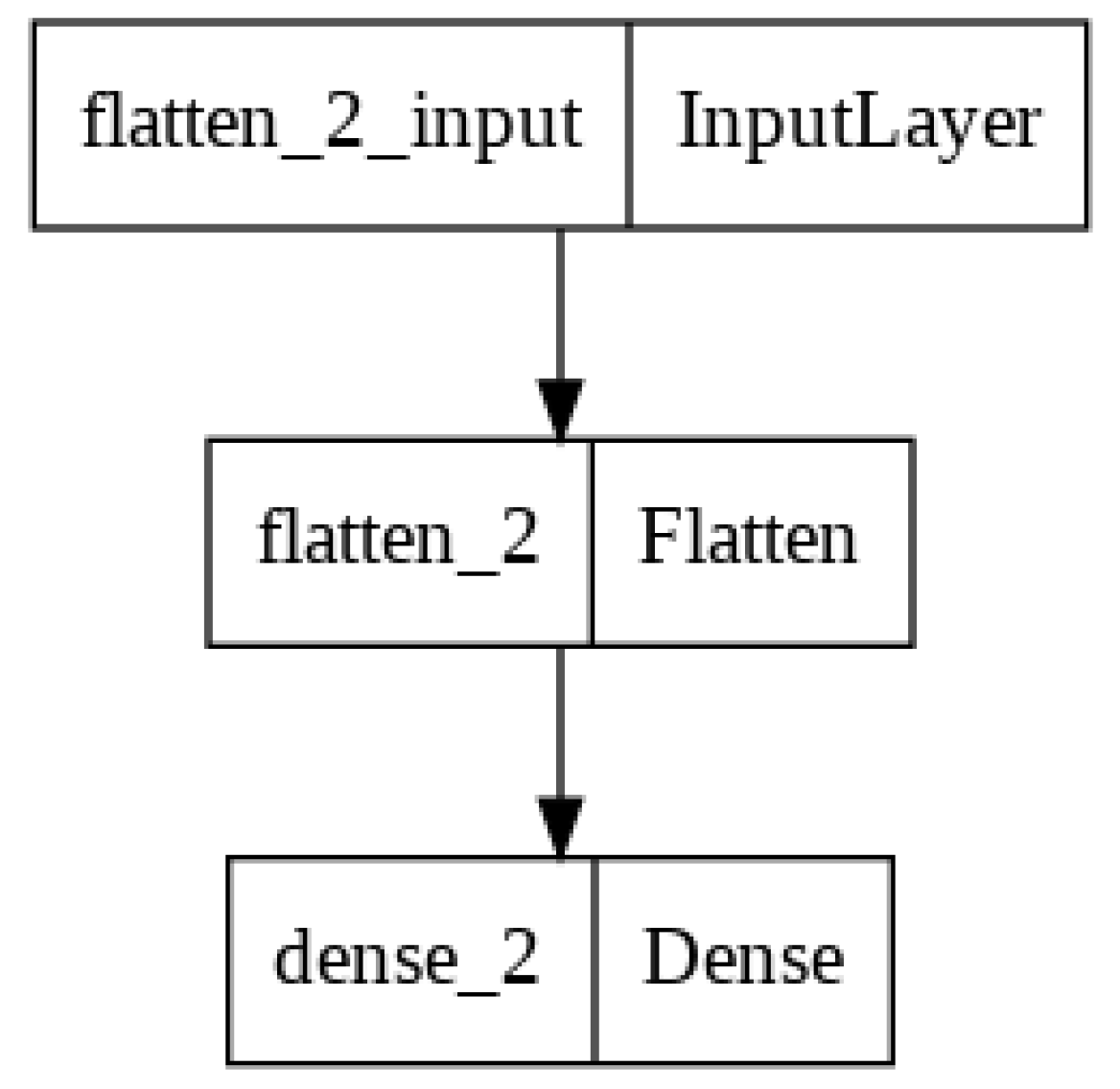
Figure 3 shows the general architecture of the quanvolutional neural network model we ultimately developed. The deployment of the model on the concentration prediction task is described below.
Unlike the simple ConvLSTM, deploying the quanvolutional neural network model required first passing the data through a quanvolutional layer before the input layer. The quanvolutional layer we developed performed convolutions on a quantum circuit accessed through the cloud. To run the quanvolutional layer, two helper functions, circuit(phi) and quanv(image), were created based on the Henderson quanvolutional neural network paper [
15].
The first function, circuit(phi), embedded data into a 4-qubit system, represented by qnode, the quantum circuit. This included embedding a layer of local rotations with angles scaled by a factor of , initiating a random circuit of , performing a measurement in the computational basis, and estimating the expectation values.
The second function, quanv(image), performed the quantum convolution, a convolution with a 2 × 2 kernel and stride of 2. This required dividing the input image into squares of 2 × 2 pixels, processing each square using the quantum circuit, and mapping the four expectation values into four different channels of a single output pixel.
The following four steps were then performed in the quanvolutional layer, as shown in
Figure 4.
The input image was embedded into a quantum circuit using circuit(phi);
A unitary operation was performed on the circuit;
The quantum circuit was measured, obtaining a classical expected value;
The convolution was performed using quanv(image), with expectations mapped to a single output pixel and the procedure iterated over the different regions of the image.
After preprocessing the data using the quanvolutional layer, the quanvolutional neural network model for concentration took inputs of 162 × 162 × 1 resolution in a 10 h window in batches of four time series. The quanvolutional neural network developed was trained on the emission concentration dataset for concentration prediction 1 and 2 h ahead. The predictions were compared to the baselines and classical ConvLSTM model using the metrics.
4. Discussion
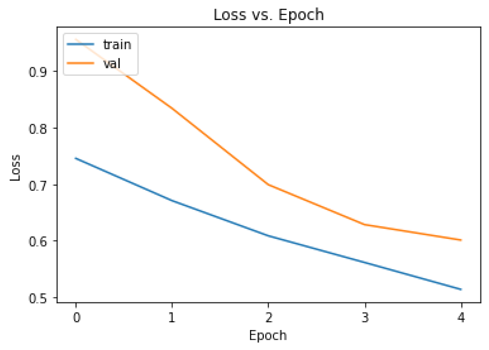
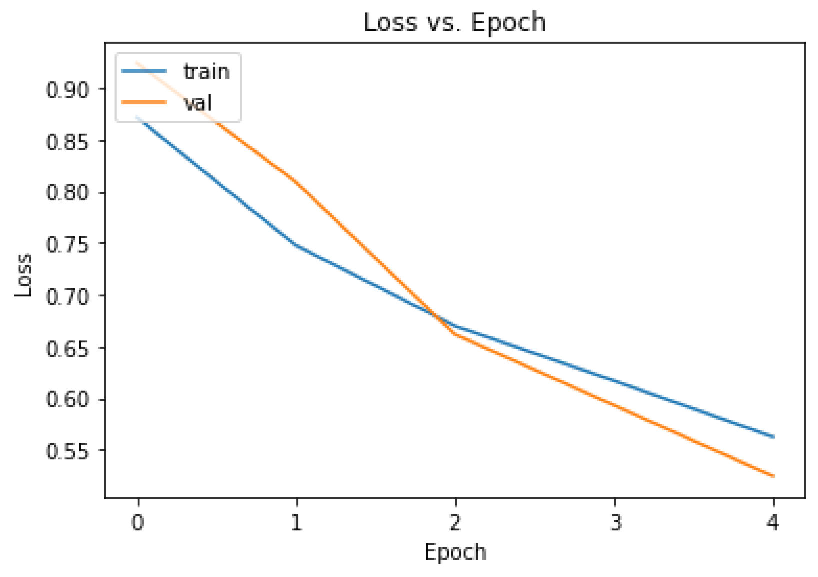
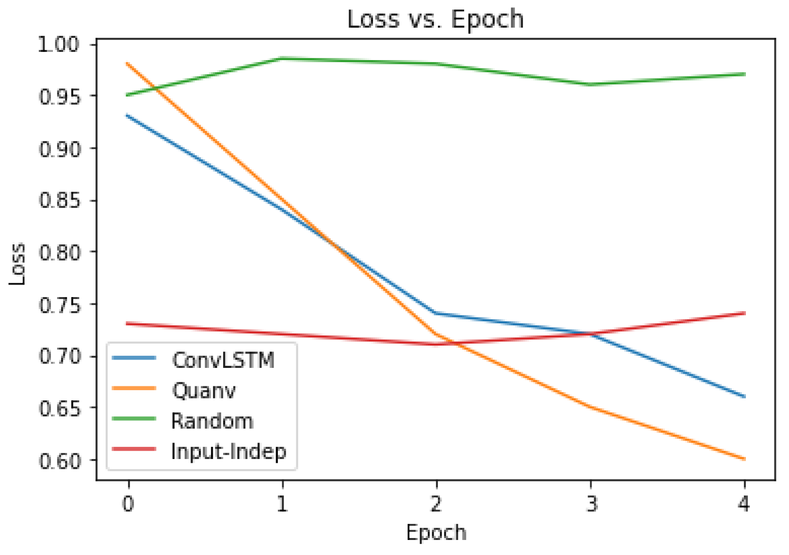
Though the classical ConvLSTM model and quantum-classical quanvolutional neural network models were intended to serve mainly as very simple tests of our evaluation framework, having kept our training and validation hyperparameters the same, we can crudely compare both models while keeping in mind that neither model is the best representative of its type. To compare, we ran both models on the reserved, unseen test dataset. We then compared the models to each other, as well as our two baselines using the evaluation framework to calculate loss (
Figure 8) and accuracy (
Table 1).
Overall, both classical and quantum-classical models were fairly similar upon evaluation, which was expected. While the classical ConvLSTM model had more complexity in terms of architecture and thus had a higher accuracy (18.9% compared to 9.5%), as seen in
Table 1, the quantum-classical model learned a simpler representation of the data due to the quanvolutional layer, resulting in better generalization to unseen data as seen in
Figure 8. Performance was better for the quanvolutional neural network model than for the ConvLSTM for both training and inference time, which were 59:66 s for training time and 1.1:1.3 s for inference. However, these times did not account for pre-processing data at around 1 min per image needed for the quanvolutional layer, which, if included, would make the classical ConvLSTM model performance faster. Both models were worse in terms of performance compared to the random chance model and input-independent model baselines, which took effectively zero seconds for training and inference time, and significantly better in terms of loss and accuracy, especially after a few epochs.
5. Conclusions
Ultimately, this work successfully demonstrates a quantum machine learning approach to emission modeling. The creation of an evaluation framework including metrics of per-pixel loss and an intersection over union accuracy, as well as baseline models, is detailed, and its usage is demonstrated to compare developed classical ConvLSTM and quantum quanvolutional neural network models. The developed models successfully generate one-hour-ahead emission concentration forecasts with lower loss and higher accuracy compared to the baselines. The ConvLSTM model successfully generated one-hour-ahead emission concentration forecasts with increasingly lower loss (6.5% and 30.5% less) and higher accuracy (18.4% and 18.6% higher) compared to the input-independent and random baseline models at the end of training. The quanvolutional neural network model successfully generated one-hour-ahead emission concentration forecasts with even lower loss (15.1% and 38.5% less) and higher accuracy (9.3% and 9.5% higher) compared to the input-independent and random baseline models at the end of training. Compared to the classical model, the quantum quanvolutional neural network model has 4% less loss and 3.7% lower accuracy. Comparison to the baseline models shows that the evaluation framework functions as expected. Additionally, though the quantum model had comparatively less accuracy compared to the classical model, the results are promising for quantum machine learning models, especially considering the limitations of this study in terms of the IoU metric used and the small number of training epochs.
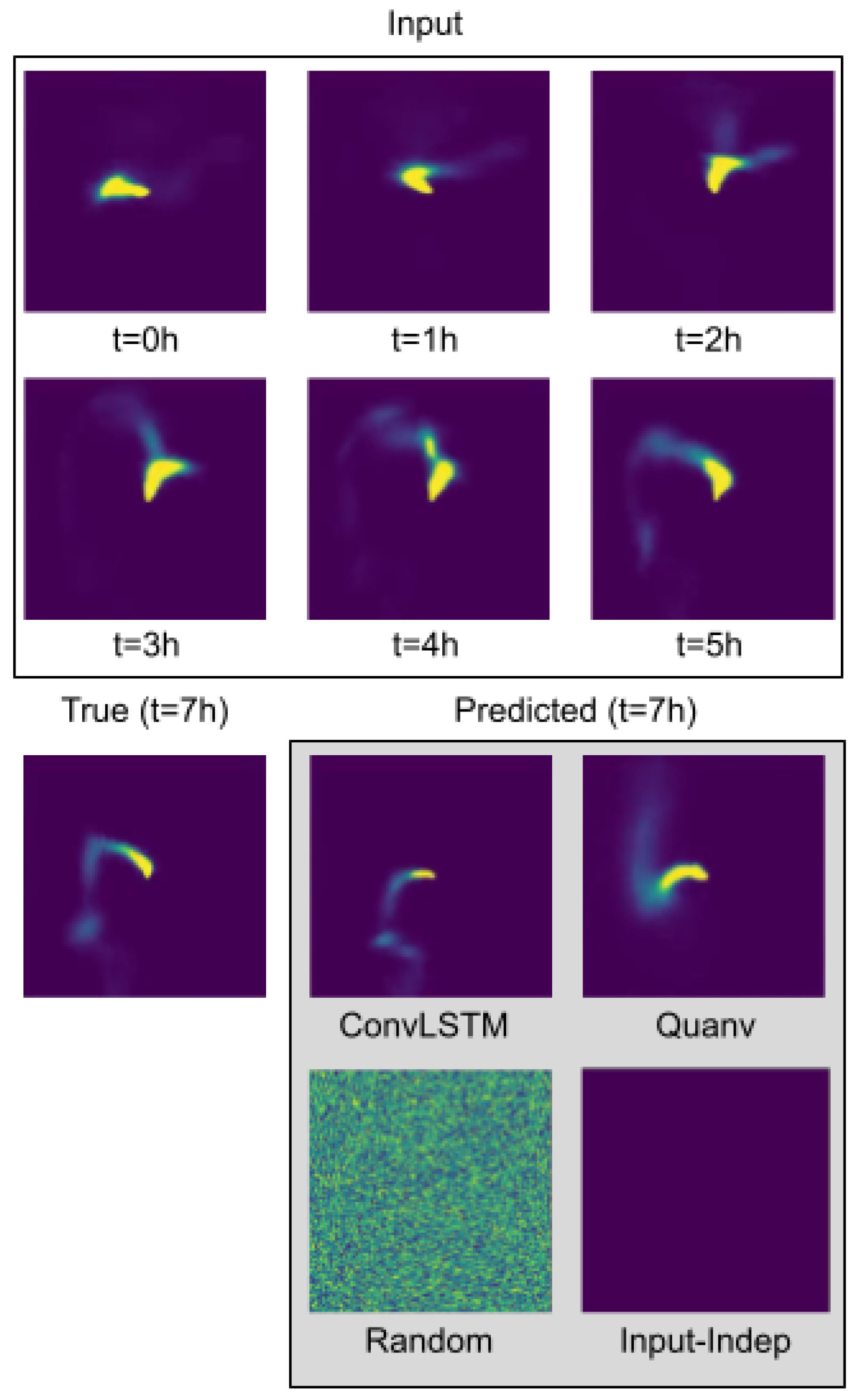
One key limitation of this work is that the evaluation framework used relies solely on the IoU metric for accuracy assessment. While IoU is a standard measure in the computer vision field, it may be too strict to fully capture the true performance of the quantum model. For example, the difference between the hour-7 predictions of the classical ConvLSTM and quantum quanvolutional neural network models were very similar in shape, as shown in
Figure 5. However, the IoUs for both the classical and quantum model were less than 20% and were even worse when predicting further in time. This was mostly due to the lack of intersection of the predictions with the true plume, not because of the incorrectness of the predicted plume shape. Therefore, measuring the similarity of plume shapes with less emphasis on intersection might be a better metric. In future work, we plan to develop a similarity of plume shape measurement to replace IoU in accuracy measurements. This could potentially lead to more meaningful evaluation of the models and more useful predictions further ahead in time.
Another limitation of this study is the small number of epochs used to train the quantum and classical models. While this small number of epochs was chosen intentionally in order to allow for a meaningful comparison between the two models, it also means that the models may not have reached their full potential. Running additional epochs would likely lead to lower loss and higher accuracy, as the models would have more opportunities to learn from the data. However, running epochs for the quantum model is extremely costly. Given our research funding, we could only afford to run 5 epochs for our quantum machine learning model. In future work, we plan to increase the number of epochs as our research funding allows, and we anticipate that this will further decrease loss and improve accuracy.
Despite these limitations, the results of this study are still promising and suggest that the quantum machine learning approach has the potential to improve emission concentration modeling. Furthermore, we believe that the quantum machine learning approach demonstrated in this work would generalize well to other datasets and emission sources. The quantum machine learning model implemented in this work is essentially just a quantum filter that pre-processes the data using the quanvolutional layer and allows the subsequent classical machine learning model to learn a different representation of the emissions outputted from the source. We believe this different representation learned following the quanvolutional layer is useful, but the effects and mechanisms behind them should be the subject of further study. Quantum machine learning is a field in its infancy and the interactions of quantum models on real-world data are far from understood. We would encourage other researchers in the field to investigate applying a quanvolutional layer to their models to test its effectiveness on their data from different domains. With further improvements, our results hint at the promise of quantum machine learning models with greater complexity trained on richer data.


