
Removal of Multiple-Radio-Frequency Interference in 1.29 GHz Wind Profiler Spectra

Abstract
:1. Introduction
2. Materials and Methods
2.1. Equipment
2.2. Data
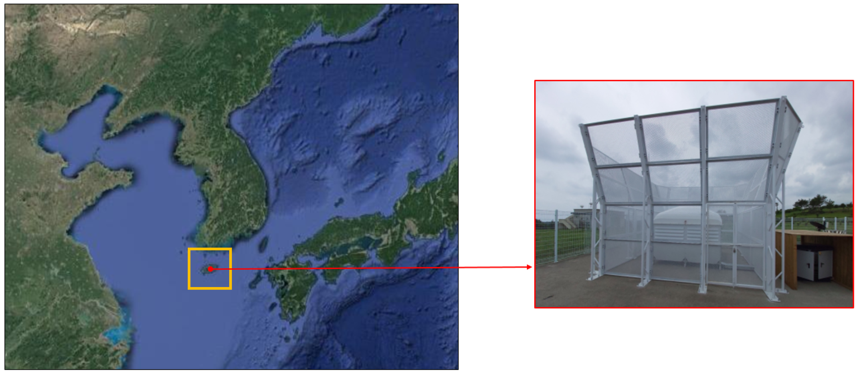
2.3. Site
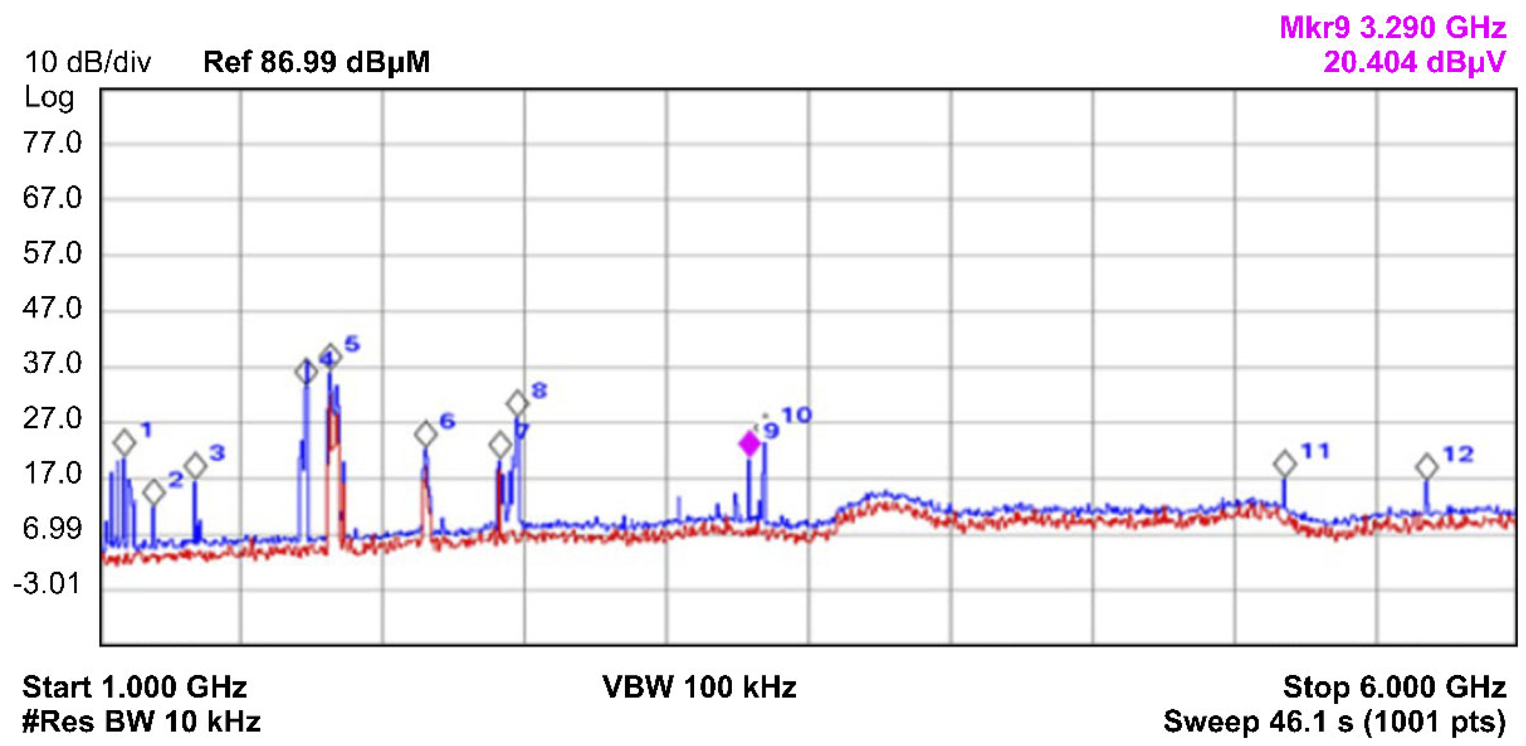
2.4. Multiple Radio Frequency Interference
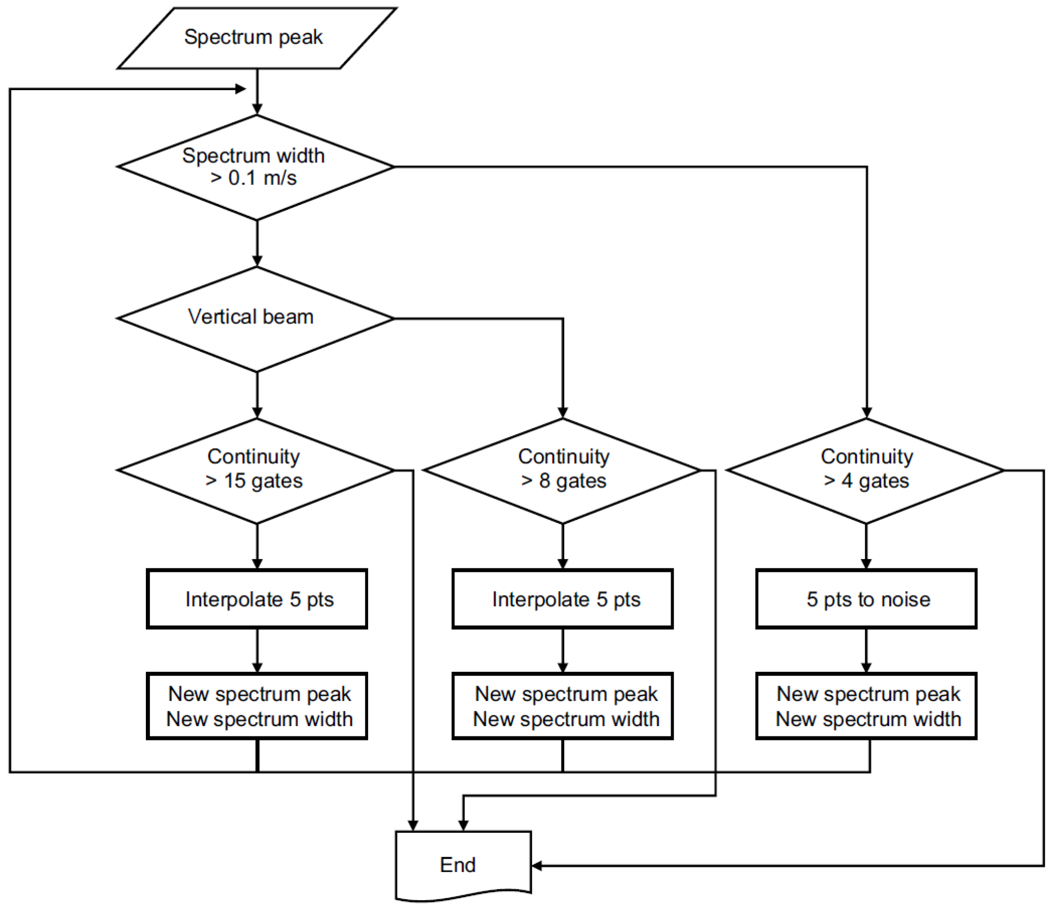
2.5. MRFI Removal Algorithm
2.6. Repeat Scanning
3. Results
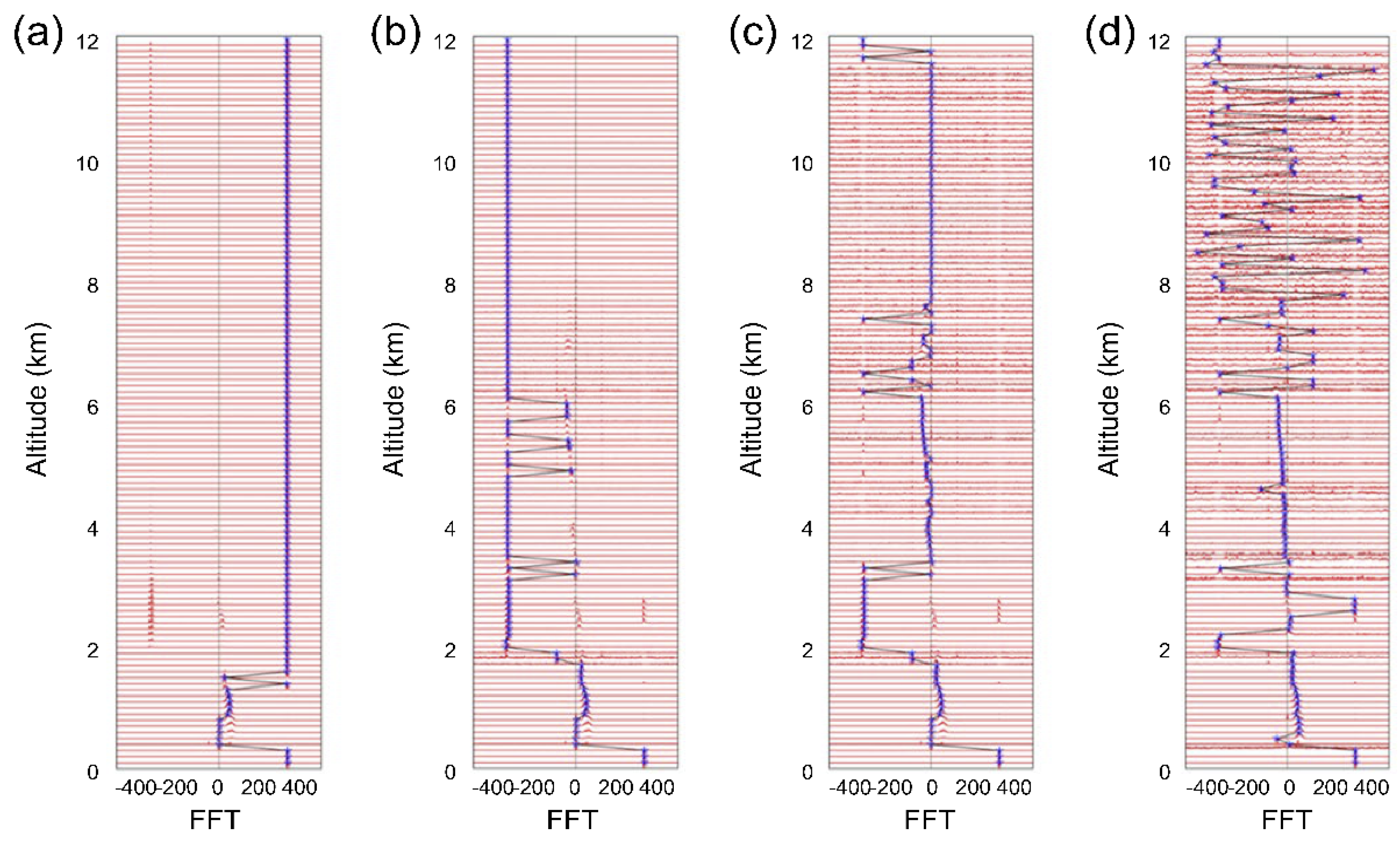
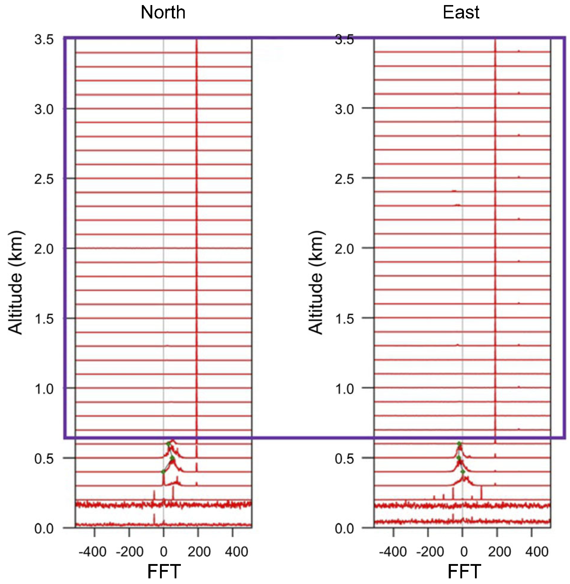
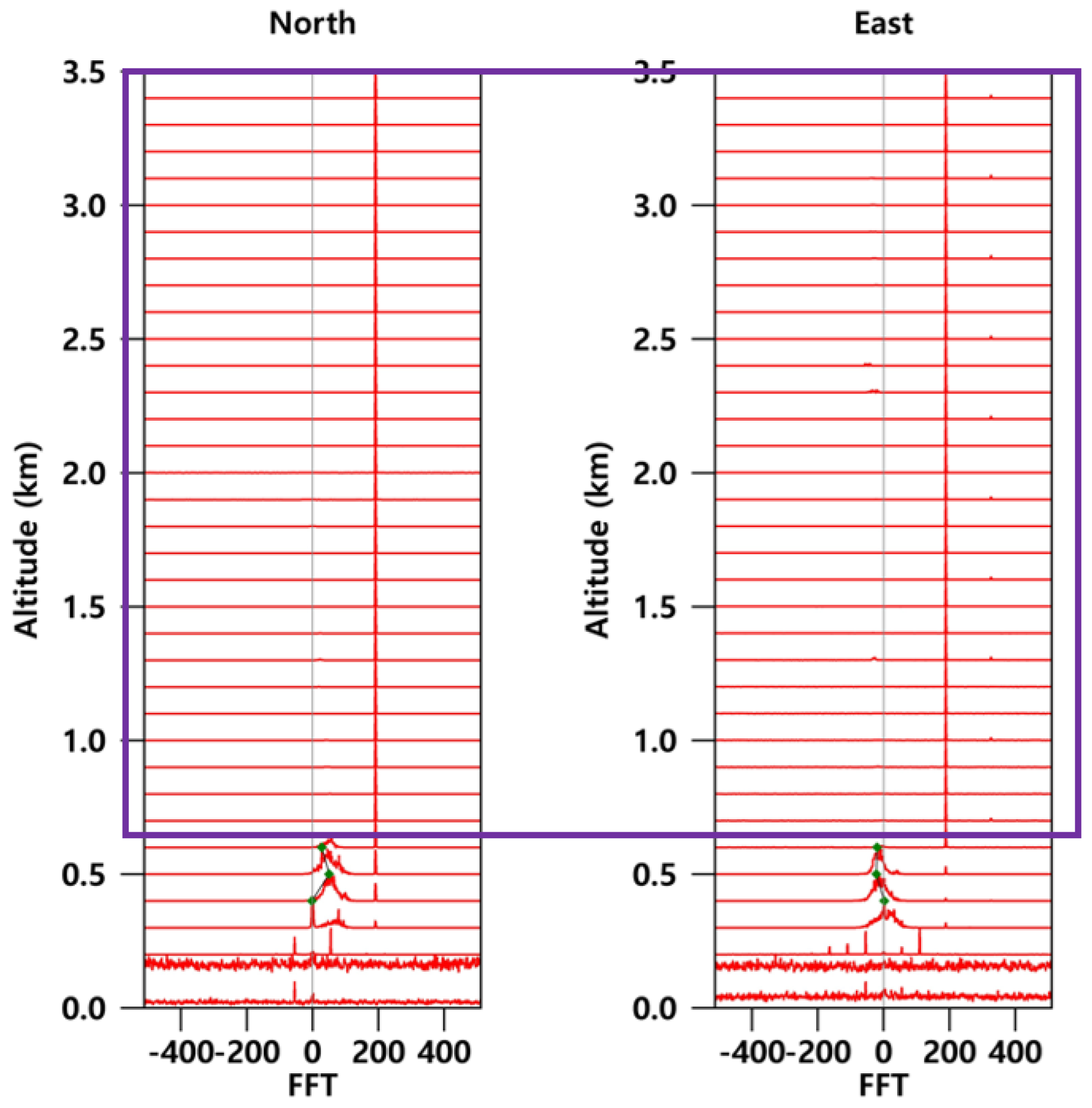
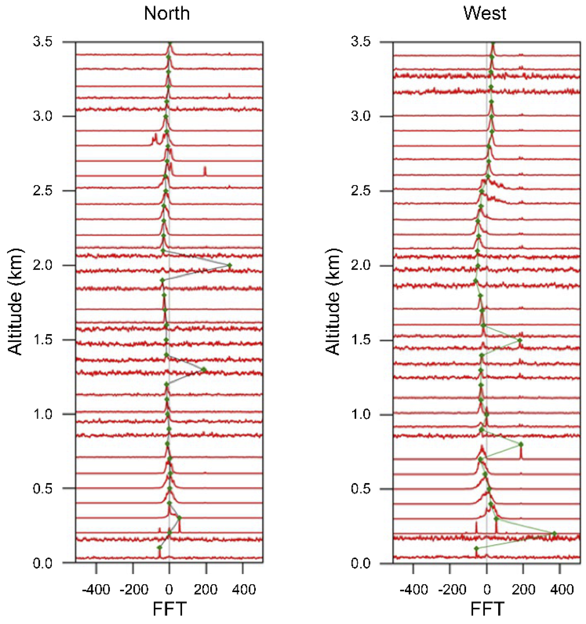
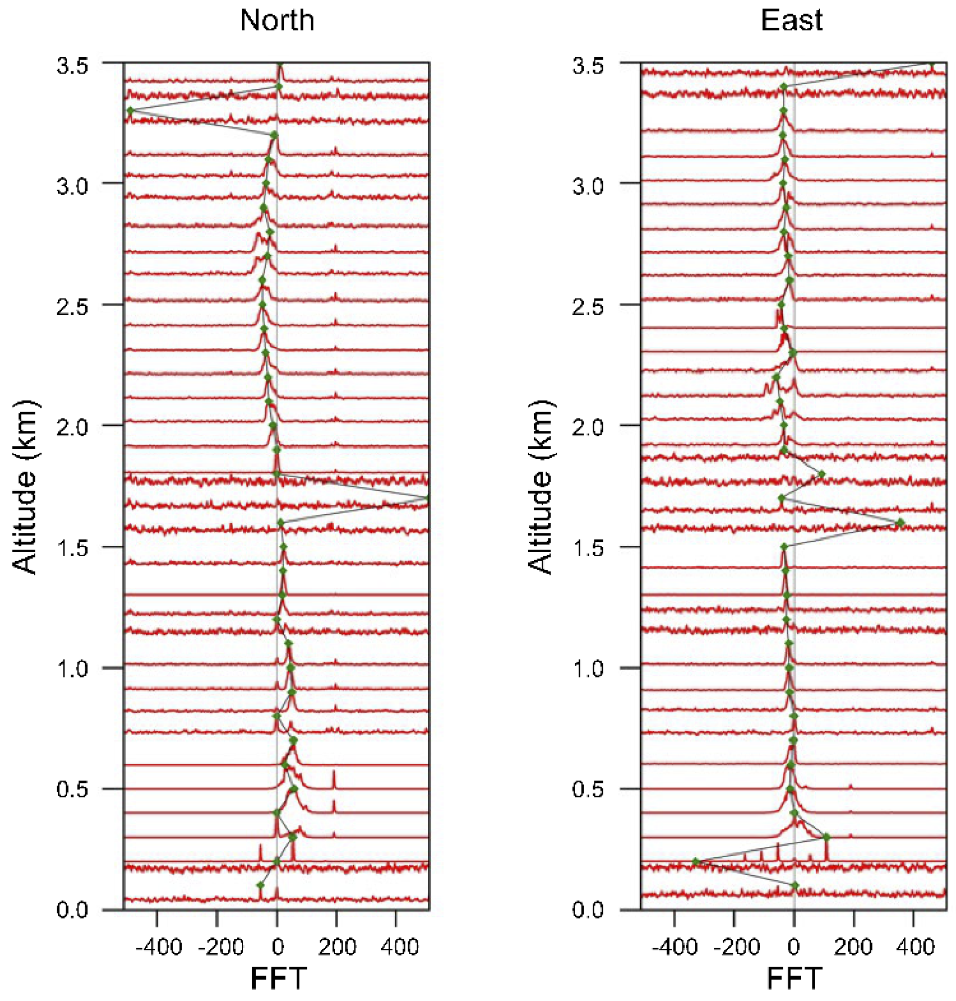
3.1. MRFI Cases
3.1.1. Case 2
3.1.2. Case 3
3.1.3. Case 11
3.1.4. Case 12
4. Discussion
5. Conclusions
Author Contributions
Funding
Institutional Review Board Statement
Informed Consent Statement
Data Availability Statement
Acknowledgments
Conflicts of Interest
References
- Brewster, K.A. Profiler Training Manual # 2: Quality Control of Wind Profiler Data; National Weather Service Office of Meteorology: Boulder, CO, USA, 1989.
- Muradyan, P.; Coulter, R. Radar Wind Profiler (RWP) and Radio Acoustic Sounding System (RASS) Instrument Handbook; U.S. Department of Energy—Office of Science: Washington, DC, USA, 2020.
- Chen, Z.; Chu, Y.; Su, C. Intercomparisons of Tropospheric Wind Velocities Measured by Multi-Frequency Wind Profilers and Rawinsonde. Atmosphere 2021, 12, 1284. [Google Scholar] [CrossRef]
- Lau, E.; McLaughlin, S.; Pratte, F.; Weber, B.; Merritt, D.; Wise, M.; Zimmerman, G.; James, M.; Sloan, M. The DeTect Inc. RAPTOR VAD-BL Radar Wind Profiler. J. Atmos. Ocean. Technol. 2013, 30, 1978–1984. [Google Scholar] [CrossRef]
- May, P.T.; Strauch, R.G. Reducing the Effect of Ground Clutter on Wind Profiler Velocity Measurements. J. Atmos. Ocean. Technol. 1998, 15, 579–586. [Google Scholar] [CrossRef]
- Muschinski, A.; Lehmann, V.; Justen, L.; Teschke, G. Advanced Radar Wind Profiling. Meteorol. Z. 2005, 14, 609–625. [Google Scholar] [CrossRef]
- Ai, W.; Huang, Y.; Hu, M.; Shen, C. Ground Clutter Removing for Wind Profiler Radar Signal Using Adaptive Wavelet Threshold. In Proceedings of the 2010 International Conference on Measuring Technology and Mechatronics Automation, Changsha, China, 13–14 March 2010. [Google Scholar] [CrossRef]
- Williams, C.R.; Maahn, M.; Hardin, J.C.; de Boer, G. Clutter Mitigation, Multiple Peaks, and High-Order Spectral Moments in 35 GHz Vertically Pointing Radar Velocity Spectra. Atmos. Meas. Tech. 2018, 11, 4963–4980. [Google Scholar] [CrossRef] [Green Version]
- Pekour, M.S. Removal of Bird Contamination in Wind Profiler Signal Spectra. In Proceedings of the 9th International Symposium on Acoustic Remote Sensing and Associated Techniques of the Atmosphere and Oceans, Vienna, Austria, 7 June–7 October 1998. [Google Scholar]
- Kretzschmar, R.; Karayiannis, N.B.; Richner, H. Removal of Bird-Contaminated Wind Profiler Data Based on Neural Networks. Pattern Recognit. 2003, 36, 2699–2712. [Google Scholar] [CrossRef]
- Jordan, J.; Leach, J.; Wolfe, D. Operation of a Mobile Wind Profiler in Severe Clutter Environments. In Proceedings of the 12th Symposium on Meteorological Observations and Instrumentation, American Meteorological Society, Long Beach, CA, USA, 8–13 February 2003. [Google Scholar]
- Electronic Communications Committee (ECC) within the European Conference of Postal and Telecommunications Administrations (CEPT). Compatibility of Wind Profiler Radars in the Radio Location Service (RLS) with the Radio Navigation Satellite Service (RNSS) in the Band 1270–1295 MHz; ECC: Lübeck, Germany, 2006; Available online: https://docdb.cept.org/download/411 (accessed on 7 January 2022).
- Lehmann, V. Use of Radar Wind Profilers in Operational Networks. In Proceedings of the WMO Technical Conference (TECO) on Meteorological and Environmental Instruments and Methods of Observation, Helsinki, Finland, 30 August–1 September 2010. [Google Scholar]
- Bollian, T.; Osmanoglu, B.; Rincon, R.F.; Lee, S.; Fatoyinbo, T. MVDR Beamforming for RFI Suppression in EcoSAR Data. In Proceedings of the EUSAR 2018: 12th European Conference on Synthetic Aperture Radar, Aachen, Germany, 4–7 June 2018. [Google Scholar]
- Tao, M.; Su, J.; Huang, Y.; Wang, L. Mitigation of Radio Frequency Interference in Synthetic Aperture Radar Data: Current Status and Future Trends. Remote Sens. 2019, 11, 2438. [Google Scholar] [CrossRef] [Green Version]
- Emery, B.; Camps, A. Introduction to Satellite Remote Sensing: Atmosphere, Ocean, Land and Cryosphere Applications; Elsevier: Amsterdam, The Netherlands, 2017. [Google Scholar]
- Wilczak, J.M.; Strauch, R.G.; Ralph, F.M.; Weber, B.L.; Merritt, D.A.; Jordan, J.R.; Wolfe, D.E.; Lewis, L.K.; Wuertz, D.B.; Gaynor, J.E.; et al. Contamination of Wind Profiler Data by Migrating Birds: Characteristics of Corrupted Data and Potential Solutions. J. Atmos. Ocean. Technol. 1995, 12, 449–467. [Google Scholar] [CrossRef]
- Lambert, W.C.; Merceret, F.J.; Taylor, G.E.; Ward, J.G. Performance of Five 915-MHz Wind Profilers and an Associated Automated Quality Control Algorithm in an Operational Environment. J. Atmos. Ocean. Technol. 2003, 20, 1488–1495. [Google Scholar] [CrossRef]
- Weber, B.L.; Wuertz, D.B. Quality Control Algorithm for Profiler Measurements of Winds and Temperatures; Wave Propagation Laboratory: Boulder, CO, USA, 1991. [Google Scholar]
- Weber, B.L.; Wuertz, D.B.; Welsh, D.C.; McPeek, R. Quality Controls for Profiler Measurements of Winds and RASS Temperatures. J. Atmos. Ocean. Technol. 1993, 10, 452–464. [Google Scholar] [CrossRef]
- Griesser, T.; Richner, H. Multiple Peak Processing Algorithm for Identification of Atmospheric Signals in Doppler Radar Wind Profiler Spectra. Meteorol. Z. 1998, 7, 292–302. [Google Scholar] [CrossRef]
- Wolfe, D.; Weber, B.; Wilfong, T.; Welsh, D.; Wuertz, D.; Merritt, D. NOAA Advanced Signal Processing System for Radar Wind Profilers. In Proceedings of the 11th Symposium on Meteorological Observations and Instrumentation, Albuquerque, NM, USA, 14–18 January 2001. [Google Scholar]
- Morse, C.S.; Goodrich, R.K.; Cornman, L.B. The NIMA Method for Improved Moment Estimation from Doppler Spectra. J. Atmos. Ocean. Technol. 2002, 19, 274–295. [Google Scholar] [CrossRef] [Green Version]
- Lehmann, V.; Teschke, G. Advanced Intermittent Clutter Filtering for Radar Wind Profiler: Signal Separation through a Gabor Frame Expansion and Its Statistics. Ann. Geophys. 2008, 26, 759–783. [Google Scholar] [CrossRef] [Green Version]
- Lehmann, V.; Teschke, G. Wavelet Based Methods for Improved Wind Profiler Signal Processing. Ann. Geophys. 2001, 19, 825–836. [Google Scholar] [CrossRef]
- Lehtinen, R.; Jordan, J. Improving Wind Profiler Measurements Exhibiting Clutter Contamination Using Wavelet Transforms. In Proceedings of the WMO Technical Conference on Meteorological and Environmental Instruments and Methods of Observation (TECO-2006), Geneva, Switzerland, 4–6 December 2006. [Google Scholar]
- Kim, M.; Kim, K.; Kim, P.; Kang, D.; Kwon, B.H. Local Wind Field Simulation over Coastal Areas Using Windprofiler Data. J. Korean Soc. Mar. Environ. Saf. 2016, 22, 195–204. [Google Scholar] [CrossRef]
- Van de Kamp, D.W. Profiler Training Manual # 1: Principles of Wind Profiler Operation; National Weather Service Office of Meteorology: Boulder, CO, USA, 1989.
- World Meteorological Organization (WMO). Guide to Meteorological Instruments and Methods of Observation, 2008 ed.; WMO: Geneva, Switzerland, 2008; Volume 2010. [Google Scholar]
- Jordan, J.R.; Lataitis, R.J.; Carter, D.A. Removing Ground and Intermittent Clutter Contamination from Wind Profiler Signals Using Wavelet Transforms. J. Atmos. Ocean. Technol. 1997, 14, 1280–1297. [Google Scholar] [CrossRef]
- Barbré, R., Jr. Development of a climatology of vertically complete wind profiles from Doppler Radar Wind Profiler systems. In Proceedings of the American Meteorological Society (AMS) Conference on Aviation, Range and Aerospace Meteorology (ARAM), Phoenix, AZ, USA, 4–8 January 2015. [Google Scholar]
- Cornman, L.B.; Goodrich, R.K.; Morse, C.S.; Ecklund, W.L. A Fuzzy Logic Method for Improved Moment Estimation from Doppler Spectra. J. Atmos. Ocean. Technol. 1998, 15, 1287–1305. [Google Scholar] [CrossRef]
- Bianco, L.; Wilczak, J.M. Convective Boundary Layer Depth: Improved Measurement by Doppler Radar Wind Profiler Using Fuzzy Logic Methods. J. Atmos. Ocean. Technol. 2002, 19, 1745–1758. [Google Scholar] [CrossRef]
- Allabakash, S.; Yasodha, P.; Bianco, L.; Reddy, S.V.; Srinivasulu, P. Improved Moments Estimation for VHF Active Phased Array Radar Using Fuzzy Logic Method. J. Atmos. Ocean. Technol. 2015, 32, 1004–1014. [Google Scholar] [CrossRef]
- Sinha, S.; Lourde, R.M.; Sarma, T.V.C. An Efficient Method of RFI and Clutter Removal in Wind Profiler Spectra. In Proceedings of the 2016 IEEE 59th International Midwest Symposium on Circuits and Systems (MWSCAS), Abu Dhabi, United Arab Emirates, 16–19 October 2016. [Google Scholar] [CrossRef]
- Hildebrand, P.H.; Sekhon, R.S. Objective Determination of the Noise Level in Doppler Spectra. J. Appl. Meteorol. 1974, 13, 808–811. [Google Scholar] [CrossRef]
- Kim, H.; Jang, M.; Lee, E. Meteor-Statistical Analysis for Establishment of Jejudo Wind Resource Database. J. Environ. Sci. 2008, 17, 591–599. (In Korean) [Google Scholar] [CrossRef]
- Yoon, H.; Jang, B. Frequency Interference, Analysis Method, and Application Examples of Sub-GHz Frequency Band. J. Korean Inst. Electromagn. Eng. Sci. 2021, 32, 1–9. (In Korean) [Google Scholar] [CrossRef]
- ISO/DIS 23032(en); Meteorology—Ground-Based Remote Sensing of Wind—Radar Wind Profiler. ISO: Geneva, Switzerland, 2022. Available online: https://dgn.isolutions.iso.org/obp/ui#iso:std:iso:23032:dis:ed-1:v1:en (accessed on 6 January 2022).
- Nguyen, L.H.; Tran, T.D. Estimation and Extraction of Radio-Frequency Interference from Ultra-Wideband Radar Signals. In Proceedings of the 2015 IEEE International Geoscience and Remote Sensing Symposium (IGARSS), Milan, Italy, 26–31 July 2015. [Google Scholar] [CrossRef]
- The Right Radar Wind Profiler for Your Application. Available online: https://library.wmo.int/pmb_ged/iom_116_en/Session%201/O1_9_McLaughlin_RightRWPforJob.pdf (accessed on 7 January 2022).
- Zhongming, Z.; Linong, L.; Xiaona, Y.; Wangqiang, Z.; Wei, L. Experience of the Japan Meteorological Agency with the Operation of Wind Profilers; World Meteorological Organization (WMO): Geneva, Switzerland, 2012; Volume 110. [Google Scholar]
- Strauch, R.G.; Merritt, D.A.; Moran, K.P.; Earnshaw, K.B.; De Kamp, D.V. The Colorado Wind-Profiling Network. J. Atmos. Ocean. Technol. 1984, 1, 37–49. [Google Scholar] [CrossRef]


| Parameter | Specification |
|---|---|
| Operation frequency | 1.29 GHz |
| Antenna type | Active phased array |
| Peak power | >1.8 kW |
| Pulse width | 0.333–10.8 μs |
| Minimum height | 150 m (dependent on pulse width, meteorological conditions, environment) |
| Maximum height | 12 km (dependent on pulse width, meteorological conditions, environment) |
| Height resolution | 50 m, 100 m (dependent on pulse width) |
| Horizontal wind speed detectable range | ±50 m/s |
| Vertical wind speed detectable range | ±20 m/s |
| Wind speed accuracy | RMSE < 1.0 m/s |
| Wind direction accuracy | RMSE < 10.0° |
| Time resolution | 10 min |
| The number of FFT (fast Fourier transform) points | 1024 |
| Number | Frequency (GHz) | Signal Power | |
|---|---|---|---|
| (db | (dBm) | ||
| 1 | 1.090 | 20.00 | −86.4 |
| 2 | 1.195 | 11.83 | −95.2 |
| 3 | 1.333 | 16.48 | −90.5 |
| 4 | 1.730 | 33.29 | −73.7 |
| 5 | 1.815 | 35.98 | −71.0 |
| 6 | 2.150 | 22.11 | −84.9 |
| 7 | 2.415 | 20.21 | −86.8 |
| 8 | 2.475 | 27.69 | −79.3 |
| 9 | 3.290 | 20.40 | −86.6 |
| 10 | 3.354 | 23.35 | −86.6 |
| 11 | 5.175 | 16.81 | −90.2 |
| 12 | 5.675 | 16.39 | −90.6 |
| Case | Date (KST) | Mode | Contaminated Beam | RFI Type | ||||
|---|---|---|---|---|---|---|---|---|
| 1 | 1st April 10:16:25 | High | East | B | ||||
| 2 | 1st April 10:57:38 | High | West | A | ||||
| 3 | 9th April 10:13:09 | High | Vertical | A, B | ||||
| 4 | 9th April 10:37:02 | High | Vertical | North | East | South | West | A |
| 5 | 9th April 10:49:05 | High | Vertical | North | A | |||
| 6 | 9th April 11:22:21 | High | Vertical | A | ||||
| 7 | 9th April 12:01:15 | High | Vertical | North | East | South | West | A |
| 8 | 9th April 12:24:43 | High | North | A | ||||
| 9 | 13th April 10:14:56 | High | North | A | ||||
| 10 | 13th April 11:38:25 | High | Vertical | B | ||||
| 11 | 13th April 11:44:14 | Low | North | West | B | |||
| 12 | 13th April 11:55:55 | Low | North | East | B | |||
Disclaimer/Publisher’s Note: The statements, opinions and data contained in all publications are solely those of the individual author(s) and contributor(s) and not of MDPI and/or the editor(s). MDPI and/or the editor(s) disclaim responsibility for any injury to people or property resulting from any ideas, methods, instructions or products referred to in the content. |
© 2023 by the authors. Licensee MDPI, Basel, Switzerland. This article is an open access article distributed under the terms and conditions of the Creative Commons Attribution (CC BY) license (https://creativecommons.org/licenses/by/4.0/).
Share and Cite
Lee, K.H.; Kwon, B.H. Removal of Multiple-Radio-Frequency Interference in 1.29 GHz Wind Profiler Spectra. Atmosphere 2023, 14, 1040. https://doi.org/10.3390/atmos14061040
Lee KH, Kwon BH. Removal of Multiple-Radio-Frequency Interference in 1.29 GHz Wind Profiler Spectra. Atmosphere. 2023; 14(6):1040. https://doi.org/10.3390/atmos14061040
Chicago/Turabian StyleLee, Kyung Hun, and Byung Hyuk Kwon. 2023. "Removal of Multiple-Radio-Frequency Interference in 1.29 GHz Wind Profiler Spectra" Atmosphere 14, no. 6: 1040. https://doi.org/10.3390/atmos14061040