Article

Outdoor Thermal Environment Regulation of Urban Green and Blue Infrastructure on Various Types of Pedestrian Walkways

1
School of Atmospheric Sciences, Sun Yat-sen University, Zhuhai 519082, China
2
Key Laboratory of Urban Meteorology, China Meteorological Administration, Beijing 100089, China
3
China Meteorological Administration Xiong’an Atmospheric Boundary Layer Key Laboratory, Xiong’an 071700, China
4
Key Laboratory of Tropical Atmosphere-Ocean System, Sun Yat-sen University, Ministry of Education, Zhuhai 519000, China
5
Guangdong Fans-Tech Agro Co., Ltd., Xi’an 710000, China
6
Department of Biological and Environmental Sciences and Technologies, University of Salento, S.P. 6 Lecce-Monteroni, 73100 Lecce, Italy
*
Author to whom correspondence should be addressed.
Atmosphere 2023, 14(6), 1037; https://doi.org/10.3390/atmos14061037
Submission received: 16 May 2023 / Revised: 5 June 2023 / Accepted: 9 June 2023 / Published: 16 June 2023
(This article belongs to the Section Biometeorology)

Abstract

:
Urban green and blue infrastructure (GBI) is effective in urban heat mitigation. However, the diurnal variations in the thermal regulation of GBI on different types of urban pedestrian walkways in the subtropical humid climate zone are unclear. Based on traverse measurements in January 2022, this study investigates how outdoor air temperature (Ta) and wet-bulb temperature (Tw) at the pedestrian level are affected by various urban morphology and GBI characteristics in the central urbanized area of Guangzhou (China). Six building-related, three vegetation-related, and three water-related parameters were applied in the analyses. Results show that green infrastructure (GI) has the strongest cooling effect (Pearson’s coefficient r = −0.33~−0.54) on Ta on cloudy evenings and the weakest cooling effect (r = −0.22~−0.32) on clear evenings. Blue infrastructure (BI) exhibits the highest correlations with the cooling effect for Ta on clear afternoons (r = −0.35~−0.51) and weaker, but more consistent, correlations throughout cloudy days (r = −0.23~−0.43). Strong correlations between GI and Tw cooling are observed in the morning and evening on clear days (r = −0.13~−0.48), while BI exhibits the strongest correlation with Tw cooling on clear afternoons (r = −0.13~−0.37). In addition, both GI and BI show a greater cooling effect on both Ta and Tw in low-rise areas compared to high-rise areas. Compared to the individual GI or BI, the integrated GBI has a higher cooling intensity for both Ta and Tw in high-rise areas. However, the cooling potential of integrated GBI is slightly lower for both Ta and Tw during noon and afternoon in low-rise areas. The findings of this study give insights into urban GBI planning and design of specific urban microclimate regulation strategies.

1. Introduction

Urbanization has caused problems such as heat waves and urban heat islands (UHI), which may cause negative health impacts and mortality [1,2]. Urban green and blue infrastructure (GBI) offers valuable ecosystem services and acts as a countermeasure to UHI and heat waves [3]. With GBI allocated in urban areas, the intra-urban microclimate is highly heterogeneous due to spatial variations in morphology, land cover, surface materials, and anthropogenic heat emissions [4,5,6,7,8]. Cycling and walking have become increasingly popular as low-carbon lifestyle choices for commuting and recreation; it is, thus, essential to improve our understanding of the heat mitigation potential of GBI on pedestrian walkways. Understanding the variations in the cooling potential of GBI across various cities and climate zones is crucial given the evolution of urbanization and climate change.
Various studies confirm that urban green infrastructure (GI) is beneficial to mitigate the UHI effect [9,10]. Street trees decrease the pedestrian level air temperature by shadowing and evapotranspiration in a limited space and continuous GI can form the so-called urban cooling island (UCI). Among various types of GI, urban parks as the major GI exhibit the particular park cooling effect (PCE) [11] and even form park cooling islands (PCI) [12]. The extent and the intensity of cooling are usually used to quantify the cooling effect of GI, which is reported to be controlled by a series of indicators such as vegetation types, the area and shape of green space, the tree coverage ratio, and the arrangement of vegetation cover, etc. [13,14,15]. A meta-analysis shows that, on average, the daytime temperature reduction is 0.94 °C based on studies covering 26 effect sizes of parks, while the nighttime temperature reduction is 1.15 °C based on 12 effect sizes [14]. Usually, GI with high tree coverage ratios is found to have greater cooling effects than those with scattered and fragmented greening and very small green spaces provide a weak cooling effect for air temperature (e.g., ~0.3 °C in London) [16]. For example, green spaces > 2 ha can reduce the surface urban heat island (SUHI) by ~2 °C in a subtropical city [17]. The overall patch shapes of green spaces also affect the cooling effect on land surface temperature (LST) [17,18]. Moreover, the background climates, e.g., the prevailing wind flow and direction, also influence the cooling effect of GI [9,19,20]. For instance, urban parks at low latitudes show greater cooling effects, and the extent of the cooling effect on canopy urban heat islands (CUHI) can range from 20 to 440 m at night depending on background meteorological conditions [20].
With high thermal inertia and through evaporative cooling, the water bodies, or the blues spaces, could provide a cooling effect of ~2.5 °C during the daytime. Similar to green spaces, atmospheric advection is also important to the cooling effect of blue spaces [21]. For example, higher wind speeds increase air mixing, which can significantly reduce the lateral cooling distribution of blue spaces [22]. The cooling effect of blue spaces depends mainly on their size and spread. Both observations and numerical modelling suggest that large waterbodies usually yield a more significant cooling effect than scattered smaller waterbodies [22,23] and simpler shapes rather than irregular shapes of waterbodies can provide a better cooling effect. Moreover, for river waterbodies, the width of the river also significantly affects the temperature and humidity of the riparian zone. The cooling effect of blue spaces varies seasonally and diurnally and the cooling effect primarily appears in the daytime, with the largest cooling effect appearing in the morning. At night, the cooling effect is insignificant and a warming effect can even appear [24], especially in summer. However, the evaporative cooling effect of blue spaces may be limited and even negate from a thermal comfort perspective since it also increases air humidity [9,22]. Furthermore, the thermal environment regulation effects of greenery and water bodies were found to be influenced by each other.
Although remote-sensing datasets with high spatial resolution have provided insights into the thermal regulation effects of GBI regarding SUHI, less accessibility to high spatial resolution near-ground air temperature datasets limits the understanding of the thermal regulation effects of GBI on CUHI [18,25]. A lack of climatological observations along commuting routes across different local climate zones (LCZs) restricted the data source and understanding, where the concept of LCZs was proposed by Stewart and Oke [26]. Most urban microenvironment assessment studies concerning GBI use data from fixed monitoring sites, but despite the high quality of these data, the spatial resolution is relatively low.
Traverse or mobile measurements of urban climate through vehicles, bicycles, or pedestrians can yield high-spatial-resolution data and complement remote sensing and fixed meteorological station-based UHI studies. In recent years, there has been an increasing number of mobile experimental campaigns for near-surface microclimate observations by vehicles, bicycles, or pedestrians carrying meteorological sensors, which can observe the spatial heterogeneity of the near-surface microenvironment in a more refined way and capture extreme values [27,28]. These mobile observation platforms are becoming increasingly convenient and flexible, allowing for the assembly of sensors and the selection of different types of loads according to specific needs. Mobile observation data could be improved by using data from fixed observation sites, that is, reducing the effect of sensor time constants to ensure the reliability of dynamic mobile observation data [29]. Furthermore, GBI is becoming more and more common in modern cities, such as lakes in urban parks and shoreline greenery along rivers. However, most existing urban thermal environment studies focus on the cooling effect of GI or BI instead of the comprehensive cooling effect of GBI, especially the studies using traverse measurements. Therefore, the diurnal variations in the thermal regulation effect of GBI and urban morphology on pedestrian walkways in different climate zones are still unclear [30,31]. More field measurement campaigns regarding the near-ground surface microclimate in the context of pedestrian walkways are needed across different climates and regions.
In this context, this study aims to investigate the temporal and spatial variation of the near-ground thermal environment along cycling routes among different LCZs. In a dense subtropical city, a mobile measurement campaign was conducted for four days from 7–10 January 2022. The mobile measurement routes covered various types of areas in the city. The study aims to answer the following research questions: (1) What are the individual impacts of GI and BI on the thermal environment along the pedestrian walkways at various times on subtropical winter days? (2) How does the integration of GI and BI affect the thermal environment along the cycling routes at different times of the day? (3) How does the thermal regulation of GBI differ under different sky conditions? To answer these questions, a methodological framework was introduced for investigating the diurnal variations in the impact of GBI on the thermal environment along pedestrian walkways by integrating multiple data sources.

2. Materials and Methods

To study the impacts of GBI on the thermal environment, the datasets of temperature and corresponding land cover and morphological parameters are necessary. The methodology framework for this study is presented in Figure 1, which can be divided into three parts: the acquisition of air temperature and wet-bulb temperature, the acquisition of land cover and morphological parameters, and the perspectives of analyses. Mobile measurements on different types of urban pedestrian walkways were conducted to capture air temperature and humidity data with geographical coordinates. The wet-bulb temperature was then calculated based on air temperature and relative humidity. On the other hand, land cover and morphological parameters were derived from GIS databases, remote-sensing indices, and street-view imagery.

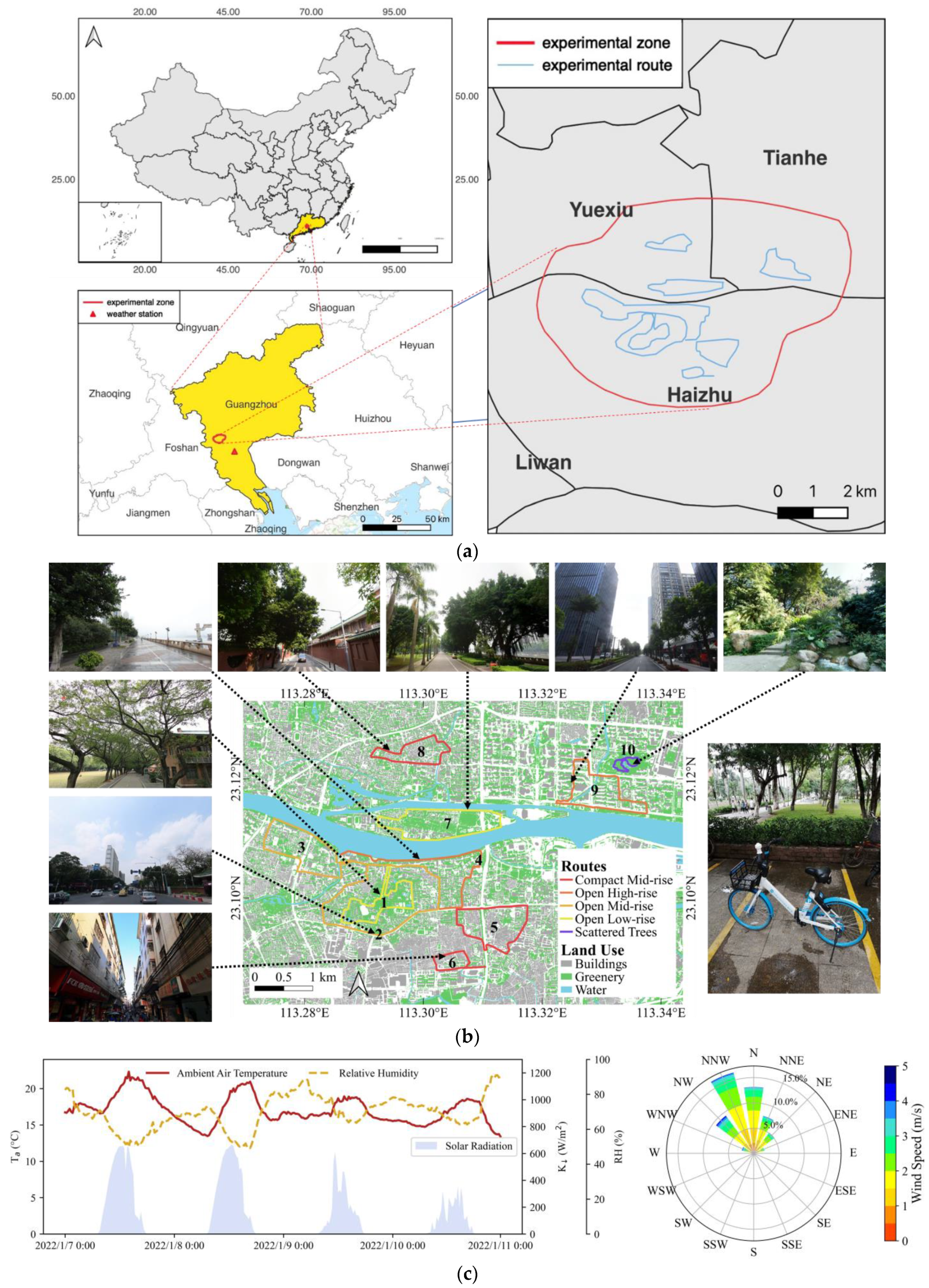
2.1. Study Site and Mobile Measurements

The traverse campaign was conducted in the center of Guangzhou city, China (23°1′ N, 113°25′ E). Guangzhou covers an area of 7434 km2 with a population of 18.81 million and has a humid subtropical climate with hot and rainy summers and warm and less rainy winters. According to Climate Bulletin of Guangzhou, 2021 [32], in 2021, the average annual temperature was 24.0 °C, the minimum and maximum air temperatures were −2.7 °C and 41.4 °C, respectively and the average annual precipitation was 1435.5 mm, featuring extreme heat, low rainfall, and severe drought. The high-temperature season lasted 151 days, with precipitation concentrated from May to October, accounting for 84% of the year. The mobile measurement routes were located near the Pearl River in the central urbanized area of Guangzhou (Figure 2a).
The traverse measurement was conducted during the period 7~10 January 2022, four times a day, covering morning (~9:00 a.m.), noon (~12:00 p.m.), afternoon (~3:00 p.m.), and night (~8:00 pm) periods. The first 2 days were clear and the last 2 days were cloudy. Ten routes that represent different LCZ types of urban pedestrian walkways were selected (Figure 2b). The LCZ types were classified by sky view factor (SVF), building surface fraction (namely, building coverage ratio, BCR, in this study), pervious surface fraction (namely, greenery coverage ratio, GCR, in this study), and height of roughness element (namely, mean height of buildings, MeanH, in this study) on traverse routes according to Stewart and Oke [26]. Notably, 10~25 m of height of roughness element is regarded as low-rise as well in this study, due to the rareness of 3~10 m height buildings in the central urbanized area of Guangzhou. The bicycle speed was controlled at 2.5~4 m/s and each traverse route took about 20 min. A tiny mobile measurement device was mounted on one handle of each bicycle (Figure 2b), with the sensors logging data every 1 s. A stationary weather station (Figure 2a) located in the suburban area about 12 km from the traverse routes was used to acquire the background weather conditions during the study period, using an IRGASON open-path eddy covariance (EC) system and logging data every 1 minute. The specific parameters of the two types of instruments are listed in Table 1. The hourly variations of background air temperature (Tastation), relative humidity (RHstation), and global irradiance are shown in Figure 2c as the hourly wind speed and direction frequency too. During the traverse measurement days, Tastation varied between 13.34 °C and 22.32 °C, and RHstation varied between 49.1% and 92.0%. The average wind speed was 1.05 m/s and the wind direction was primarily north north-west (NNW).

2.2. Land Cover and Morphological Parameters

2.2.1. Coverage Ratios of Building, Greenery, and Water

Various land cover and morphological parameters can reflect urban land cover and morphology in outdoor thermal environment studies. These parameters can be either two-dimensional (2D) or three-dimensional (3D), derived from a geographic information system (GIS) database or using remote-sensing indices as proxies. Moreover, since this study focuses especially on pedestrian walkways, 3D spatial parameters developed from street views are also considered. To describe the land cover and morphological parameters for each point along the mobile measurement routes, zonal averages of these parameters within a circular buffer were associated with each sampling point on the routes (Figure 3).
The specific coverage ratios include building coverage ratio (BCR), greenery coverage ratio (GCR), and water coverage ratio (WCR), which are 3 types of 2D land fraction parameters that reflect landcover characteristics. They were derived from the GIS landcover database of the central urbanized area of Guangzhou provided by Shi et al. [33]. The database was derived from the GeoEye-1 satellite imagery obtained on 22 October 2017, including 7 landcover categories: building, impervious, bare land, grass, shrub, tree, and water body. The projected coordinate system was unified as WGS_1984_UTM_zone_49 N. Based on the database, grass, shrub, and tree were all considered vegetation. BCR, GCR, and WCR are the area proportion of buildings, vegetation, and water bodies in each circular buffer, respectively. In addition, DistW is a 2D spatial parameter that is the distance to water bodies.
Floor area ratio (FAR) and mean height of buildings (MeanH) are two 3D spatial parameters that describe urban morphology. FAR is the ratio of the total floor areas in each buffer to the buffer area, and MeanH is the ratio of the area-weighted average of the height of buildings in each buffer to the buffer area [35].

2.2.2. Remotely Sensed Green and Blue Indices

Sentinel-2 satellite images were used to derive GBI-related parameters based on the surface spectral reflectance. The normalized difference vegetation index (NDVI) and the normalized difference water index (NDWI) were used as indicators to reveal the vegetation and water characteristics of the land:
NDVI = (NIR − red)/(NIR + red),
NDWI = (NIR − MIR)/(NIR + MIR).
The calculation of these indices was based on the absorption of various light wavelengths by the green and blue surfaces. Specifically, the NDVI and NDWI highlight higher reflectance in the near-infrared spectral range (NIR), using green, red, NIR, and mid-infrared spectral range (MIR) bands of different wavelengths to calculate the two indicators for all pixels in the selected images. The normalized difference built-up index (NDBI) was also used as an additional index to represent the degree of built-up land. This index highlights urban areas with higher reflectance in the shortwave infrared spectral range (SWIR) and is calculated as follows:
NDBI = (SWIR − NIR)/(SWIR + NIR).

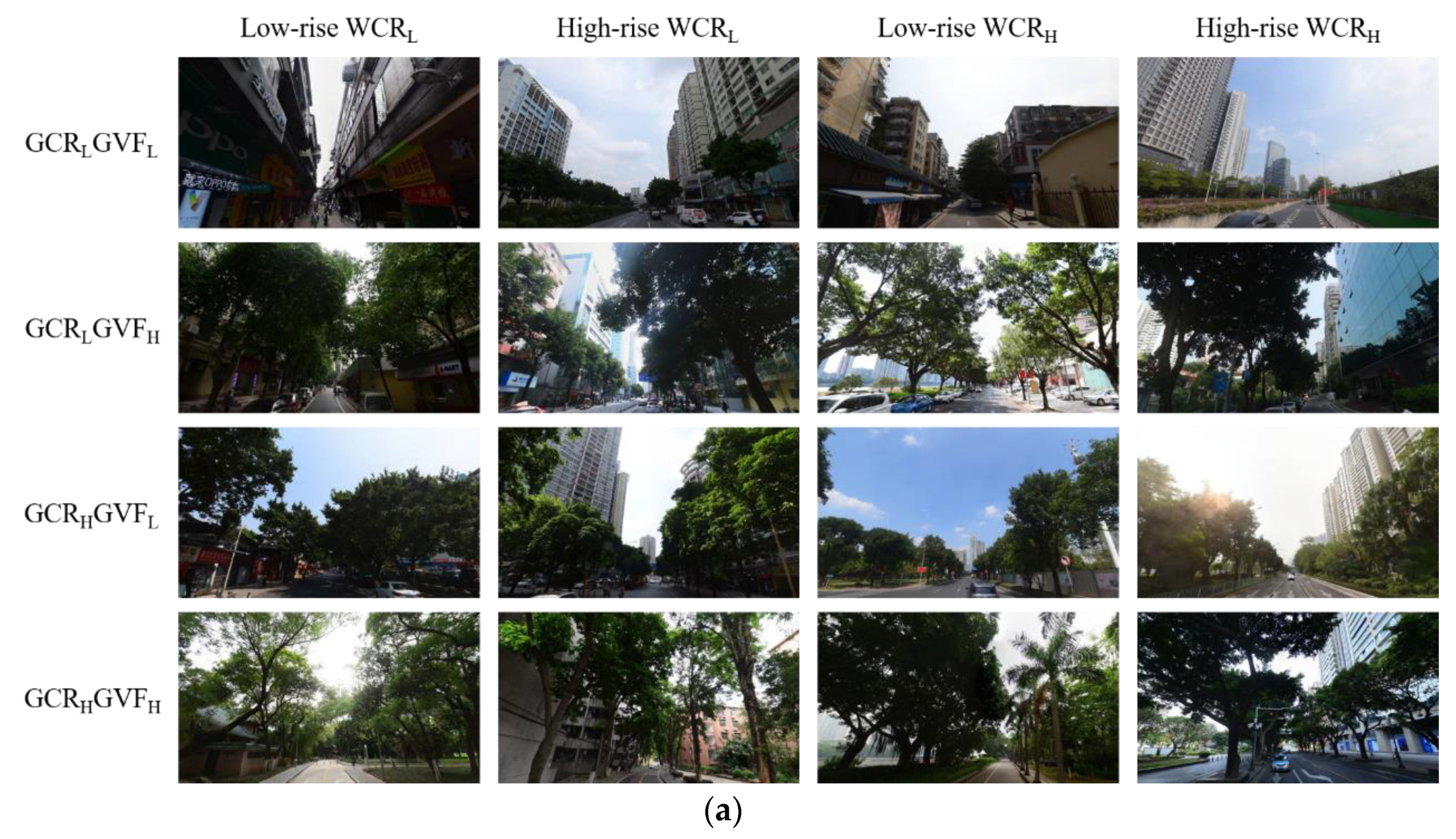
2.2.3. Street-View Factors

Emerging research has investigated the potential of traverse surveys for analyzing near-surface thermal environments along pedestrian routes at the microscale. Unique to corridor environment, the street-view imagery along routes provides detailed 3D morphological information and has become a useful morphological indicator in urban micro-environment studies. Results from these studies indicate that regression models utilizing 3D features derived from street-view images can exhibit comparable performance to conventional land-use regression (LUR) models based on GIS database-derived parameters [36,37]. Among these street-view-derived 3D features, view factors such as sky-view factor (SVF), building-view factor (BVF), and greenery-view factor (GVF) are most frequently studied and can be obtained using semantic segmentation with deep learning techniques [38,39]. SVF is commonly expressed as a unitless value ranging from 0 to 1, where 0 implies complete obstruction of the sky by obstacles and 1 indicates an unobstructed sky view [40]. BVF and GVF can be similarly defined. The calculation method for view factors is explained in previous works [41,42,43].
In general, the parameters have been here classified into three categories, namely, building-related parameters, vegetation-related (green infrastructure) parameters, and water-related (blue infrastructure) parameters. Among them, NDBI, BCR, NDVI, GCR, NDWI, WCR, and DistW are the landcover (2D) parameters and FAR, MeanH, BVF, SVF, and GVF are the morphology (3D) parameters.

2.3. Wet-Bulb Temperature

The wet-bulb temperature (Tw) is an important heat stress index, referring to the temperature at which wet air mass reaches saturation through adiabatic cooling under the condition of constant air pressure. It can directly reflect the heat transport between the human body and the ambient air by perspiration. When the ambient Tw is higher than the human skin temperature, the human body cannot dissipate heat, resulting in heat stress [44]. In this study, the Tw was obtained from the following equations:
es = 6.122 exp [(Ta × 17.67)/(Ta + 243.5)]     (Ta < 0),
es = 6.1078 exp [17.2693882 × (Ta + 273.15 − 273.16)/(Ta + 273.15 − 35.86)]     (Ta > 0),
es,w = 6.1078 exp [17.2693882 × (Tw + 273.15 − 273.16)/(Tw + 273.15 − 35.86)],
ea = es × RH/100,
ea = es,w − 0.000660 (1 + 0.00115 Tw) (TaTw) P.
where es represents the saturated water vapor pressure in the air (hPa); ea represents the actual water vapor pressure in the air (hPa); Ta, RH, and Tw represent the air temperature (°C), relative humidity (%), and wet-bulb temperature (°C), respectively; P is the standard sea level pressure of 1013.25 hPa; and es,w represents the saturated water vapor pressure (hPa) calculated by Tw. Equation (4) is recommended by the World Meteorological Organization (WMO) [45]. Equation (7) was proposed by Moratiel et al. [46]. In this study, ΔTa and ΔTw are used, which represent the difference between Ta (or Tw) in urban areas (data on traverse routes) and suburban areas (data from the stationary weather station). The data from the stationary weather station with a time resolution of 1 min is interpolated into 1 s to match the data on traverse routes.

3. Results

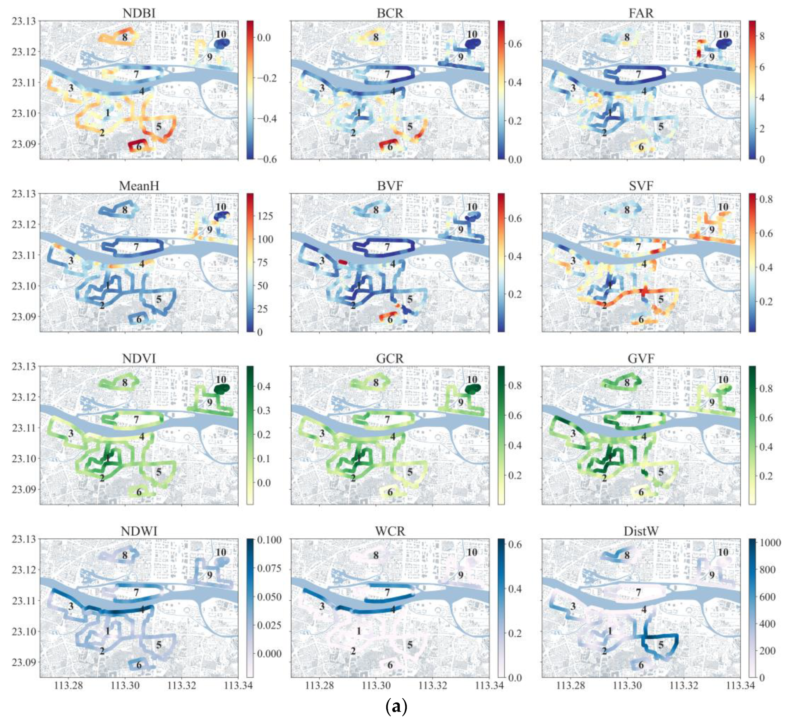
3.1. Land Cover and Morphological Characteristics across the Routes

To clarify the spatial variability of the land cover and morphological characteristics on the traverse routes, Figure 4a shows the spatial distributions of the twelve examined urban morphological and land cover parameters along the mobile measurement routes. The 10 sample routes vary significantly in their land cover and morphological parameters, highlighting the diversity of the urban environment. NDBI and BCR indicate the built-up intensity within a given area. Routes five, six, and eight are within compact mid-rise areas, featuring high NDBI and BCR. The routes with the highest NDBI, BCR, and lowest GCR (23.090~23.095° N, 113.30~113.32° E) are traversing the urban villages (routes five, six). The urban village is a unique feature of the urban landscape in Guangzhou. These villages are areas that have been transformed from rural communities into densely populated urban areas, often as a result of rapid urbanization and economic development. Despite their location within the city, urban villages tend to have a distinct character and culture. They are typically characterized by a mixture of high-rise apartment buildings and low-rise housing, small shops and markets, and narrow, winding streets with minimal GI.
Route one and route ten are characterized by high values of NDVI and GCR, which measure the proportion of green space within a given area. Route one is situated inside a university campus (23.095~23.105° N, 113.285~113.300° E) and route ten is within an urban park (23.120~23.125° N, 113.330~113.335° E), both of which are covered with big tall trees.
Routes four and seven experience high NDWI and WCR values, which measure the relative abundance of water bodies and the adjacency to water bodies, respectively. Route seven is located on the island in the center of the Pearl River and the route circles the island. This route also experiences the lowest BVF and high GVF. However, compared with route four, a large part of which is along the southern Pearl River bank (23.105~23.115° N, 113.27~113.31° E) flanked by tall buildings (featured by high MeanH), the buildings along route seven are mostly low-rise. Route nine is along a green belt nearby the Pearl River, but has relatively lower NDWI and WCR.
Figure 4b shows the frequency distributions of the urban morphological and land cover parameters along the mobile measurement routes, most of which are not normally distributed. The optimal sizes of buffers are determined by the results of the Pearson correlation analysis, which are shown in Section 3.4. Eventually, 30 m for NDBI, NDVI, and NDWI; 500 m for BCR, FAR, and WCR; 100 m for MeanH; 20 m for GCR; and 50 m for BVF, SVF, and GVF were applied. The median values of BCR and GCR for all sampled routes are 0.2265 and 0.4816, respectively.
Since the number of areas would be doubled with each additional parameter used for division, MeanH, GCR, GVF, and WCR were chosen eventually on the premise of ensuring distinctive urban morphology and GBI (Figure 5a). The subscript “L” indicates the data lower than the median and the subscript “H” indicates the data higher than the median. The routes are firstly classified into two main classes: low and high WCR (WCRL and WCRH), distinguishing the BI situations. Then WCRL and WCRH classes are further classified according to the MeanH, GCR, and GVF characteristics, considering there could be large differences between GCR and GVF values because they feature 2D and 3D greening characteristics, respectively. Figure 5b examines the inter-class differences in BCR, NDBI, WCR, and NDWI. BCR and NDBI differ with GCR levels for low-rise areas and WCRH high-rise areas. Since higher GCR inevitably means lower BCR or NDBI, and this trade-off is common in any city, the differences are within acceptable limits. Moreover, BCR is generally higher in high-rise areas than in low-rise areas, unless both WCR and GCR are low, revealing a positive correlation between the height and density in most cases except for the areas that lack GBI. The similarity of WCR and NDWI with different GCR and GVF levels is ensured in WCRL areas, but the variability is exhibited when in WCRH areas. The median of WCR is extremely low in low-rise WCRH areas while GCR is high but GVF is low, therefore, this case can be considered to be away from water bodies, to some extent. WCR is generally higher with lower GCR and higher GVF in low-rise WCRH areas, however, lower with the above GI conditions in high-rise WCRH areas, which may be due to the existence of the greenbelt along the river in high-rise areas. NDWI in WCRH areas is higher when GI is lusher, especially higher GVF in low-rise areas and higher GCR in high-rise areas.

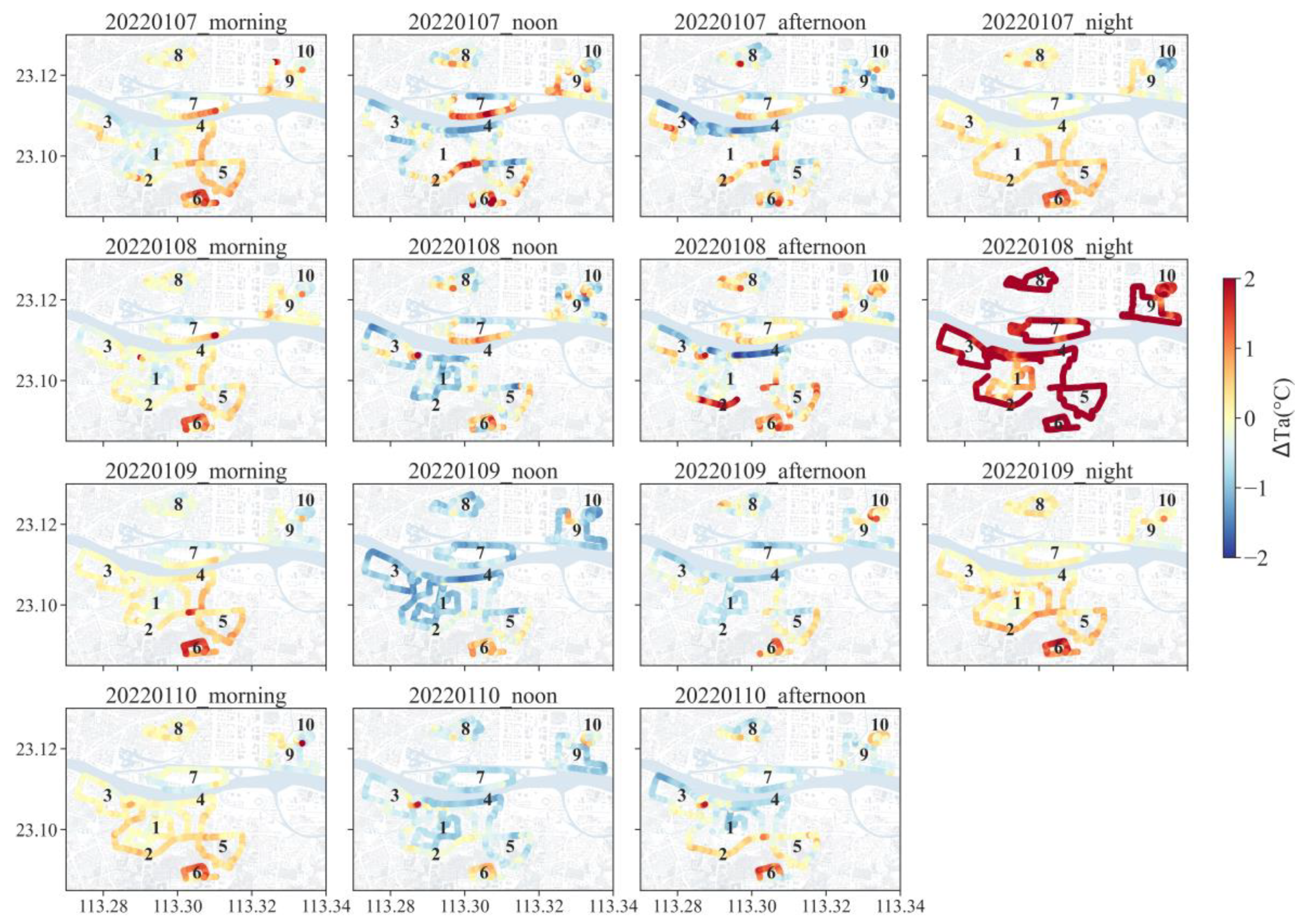
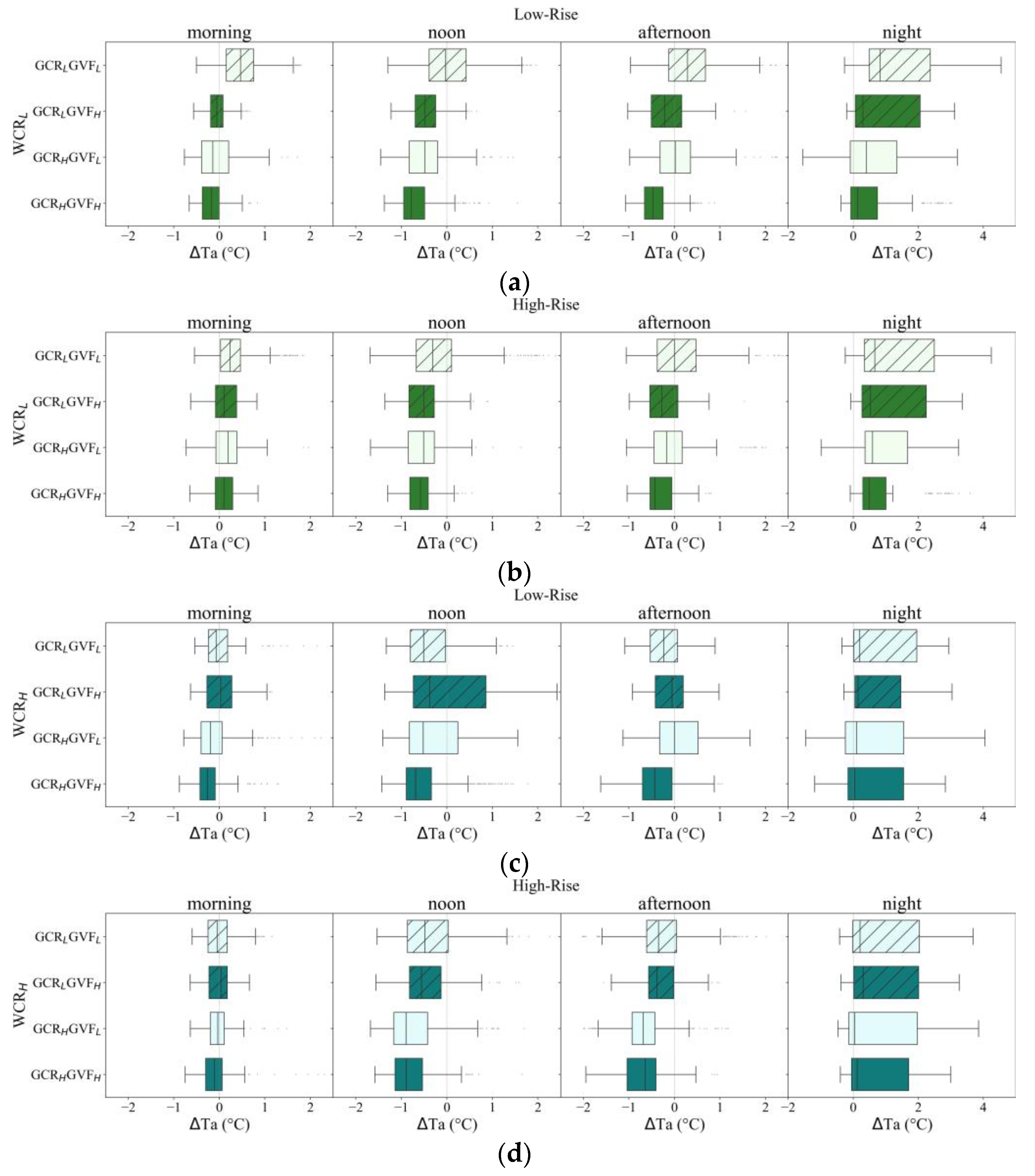
3.2. Spatial Distribution of Route-Suburban Temperature Difference (ΔTa) along the Routes

The spatial distribution of the thermal environment on the traverse routes is affected by the land cover and morphological characteristics. Figure 6 depicts the spatial distribution and variability of ΔTa (temperature difference between the routes and the suburban fixed station) along the mobile routes during the experimental period. Overall, the temperature along the routes in the urban village with low vegetation (route six) is the highest among all types of routes during the whole day. In contrast, the routes inside the urban park (route ten) and the highly vegetated campus area (route one) exhibit the lowest ΔTa. In the near-water region, ΔTa along the route on the northern bank of the river on the island (route seven) is relatively high compared to all other measurement routes. On the contrary, the traverse routes along the southern bank of the river (route four) exhibit relatively low ΔTa among all examined routes.
Regarding the diurnal cycle, ΔTa during the morning and night periods is higher than during the noon and afternoon periods. During the night, ΔTa is even slightly higher than in the morning period, especially for the clear evening on 8 January, when ΔTa exceeds 2 °C in most areas. This indicates that during the transitional nighttime from a clear day to a partially cloudy day, abnormal high ΔTa may be shown because of more sensible heat flux at the nighttime induced by the higher heat storage of impervious materials in the urban area on clear daytime and with the heat trapped due to the poorly ventilated building canyons, eventually cooling down to an ambient Ta more slowly than the suburban area. On the following partially cloudy day, both the urban and suburban areas fully release the heat storage on the last clear day, therefore, showing slight ΔTa differences in the morning and evening between 8–9 January.
The spatial distributions of ΔTa during the first two clear days and the second two cloudy days show apparent differences during the noon and afternoon periods, but slighter differences in the morning and evening. During the noon and afternoon experimental periods, all routes show greater spatial heterogeneity on clear days than on cloudy days. For noon and afternoon periods on the two cloudy days (9–10 January), negative ΔTa occurs on most routes, including the routes traversing the old town district (route seven), the new town district (route nine), the highly vegetated campus (route one) and urban park area (route ten), as well as the routes along the river (route four). However, for 3 days during our traverse campaign, the urban park exhibits positive ΔTa during the afternoon period, indicating that the cooling effect of urban parks is not significant in the afternoon in winter.
The ΔTa distribution in various types of traverse routes classified by MeanH, WCR, GCR, and GVF are shown in Figure 7. As detailed in Figure 5, the parameters higher than their medians are called high-rise, WCRH, GCRH, and GVFH, otherwise low-rise, WCRL, GCRL, and GVFL. For each combination of MeanH and WCR, the highest and lowest ΔTa generally appears in GCRLGVFL and GCRHGVFH, respectively.
Considering the thermal regulation of GI in areas with a small amount of blue infrastructure (BI), with the WCRL results, GI shows a stronger cooling effect in low-rise areas rather than high-rise areas over the four measurement days. In low-rise WCRL areas, ΔTa is negative as long as GCR or GVF is high during the morning and noon traverses (Figure 7a). The cooling intensity among these situations is 0.52~0.63 °C and 0.45~0.75 °C in the morning and at noon, respectively, compared with the reference type GCRLGVFL, which represents areas with little GI (Table 2). However, in high-rise WCRL areas, the median ΔTa is positive in all cases in the morning and negative in all cases at noon. Compared to GCRLGVFL (median ΔTa = −0.31 °C) as a reference, the cooling intensity from GI reaches 0.04~0.14 °C in the morning and 0.20~0.27 °C at noon. In the afternoon, ΔTa in GCRLGVFH is negative and lower than that in GCRHGVFL for both low-rise and high-rise areas, indicating that the shading from the tree canopy could be the main cooling mechanism rather than evapotranspiration. In the evening, the ranges of ΔTa are narrower while GCR is high, especially in GCRHGVFH, demonstrating the role of GI in stabilizing Ta at lower values at night. The cooling intensity of GI in low-rise areas is 0.27~0.76 °C and 0.42~0.69 °C in the afternoon and evening, respectively, compared to the baseline of GCRLGVFL. In high-rise areas, the cooling intensity of GI is 0.17~0.43 °C and 0.07~0.18 °C in the afternoon and evening, respectively.
As shown in Figure 7c,d, the integration of GI and BI does not always result in better cooling than using one of them alone. In WCRH areas, GCRLGVFH shows the highest median ΔTa in low-rise areas during the morning and noon and in high-rise areas in the morning and evening. GCRHGVFL within the low-rise WCRH category does not cool the air in the afternoon (Figure 7c). The cooling intensity of BI is 0.48~0.63 °C in low-rise areas and 0.17~0.46 °C in high-rise areas, with the highest cooling in the evening and the lowest at noon (Table 2). In high-rise WCRH areas, the cooling intensity of different GVF levels but the same GCR level are similar during noon and afternoon, indicating that GCR is a key factor in air cooling in high-rise waterfront areas during noon and afternoon (Figure 7d). Whether in low-rise or high-rise areas, waterfront ΔTa exhibits little difference among various types of GCR and GVF in the evening, revealing that while GI can contribute to cooling, its role in reducing ambient air temperature may not be evident with the existence of large BI. However, this result depends on various factors of GI and BI, such as their size, type, density, and placement, as well as the atmospheric conditions.
Comparing the two low-rise areas with different WCR levels, the maximum cooling intensity of GI alone from the morning to evening is 0.63 °C, 0.75 °C, 0.76 °C, and 0.69 °C, respectively, and the maximum cooling intensity of GBI is 0.73 °C, 0.66 °C, 0.72 °C, and 0.78 °C, respectively. It illustrates that in low-rise areas, GI alone may sufficiently cool the air in the morning and evening. However, during noon and afternoon, the addition of BI reduces the cooling intensity of GI.
Comparing the two high-rise areas with different WCR levels, the maximum cooling intensity of GI from the morning to evening is 0.14 °C, 0.27 °C, 0.43 °C, and 0.18 °C, respectively, and the maximum cooling intensity of GBI is 0.35 °C, 0.59 °C, 0.69 °C, and 0.62 °C, respectively. This indicates that in high-rise areas, on the other hand, the addition of BI helps cool the air more effectively with sufficient GI, especially at noon and in the evening.

3.3. Spatial Distribution of Route-Suburban Temperature Difference (ΔTw) along the Routes

As a more direct indicator of heat stress, it is crucial to figure out the relationship between the spatial distribution of Tw and the spatial distribution of land cover and morphological parameters. Figure 8 shows the spatial variation of ΔTw during the morning, noon, afternoon, and evening measurement periods. The urban village (route six) is generally the highest ΔTw area and the roads with high SVF (routes two and seven) present high ΔTw during the noon and the afternoon on clear days as well. In the morning, the spatial variations of ΔTw are smaller than that of ΔTa. On clear days, the lowest ΔTw might appear in the morning, while on cloudy days, the highest ΔTw might appear in the same period. Different from the ΔTa distribution, during the noon and the afternoon, areas with negative ΔTw are rare and could not even be found on clear days, indicating that the whole urban area plays a role in heating wet-bulb temperature. In general, ΔTw in the morning is higher on cloudy days, but during the noon, afternoon, and evening it is higher on clear days.
The ΔTw distribution in various types of traverse routes classified by MeanH, WCR, GCR, and GVF is shown in Figure 9. The medians of ΔTw in most of the cases from noon to night are positive, which is different from the generally negative ΔTa during noon and afternoon (Figure 7).
In WCRL areas, high ΔTw appears during the afternoon and evening and GI generally reduces ΔTw (Figure 9a,b). Compared to high GVF, high GCR does not provide a significant cooling effect in low-rise areas during the day (Figure 9a). During the morning, noon, afternoon, and evening, the cooling intensity of GVF reaches up to 0.37 °C, 0.33 °C, 0.38 °C, and 0.55 °C in low-rise areas and 0.09 °C, 0.15 °C, 0.16 °C, and 0.09 °C in high-rise areas, respectively, suggesting that GVF has a stronger cooling effect for Tw in low-rise areas rather than high-rise areas while far from water bodies (Table 3). In the evening, the spatial variations of ΔTw with high GCR or GVF are slightly smaller than in GCRLGVFL, demonstrating that GI is slightly helpful in stabilizing inland Tw at nighttime.
In WCRH areas, the spatial variations of ΔTw are smaller in high-rise areas than in low-rise areas (Figure 9c,d). The cooling effect of BI is small, where the greatest Tw cooling intensity in low-rise and high-rise areas is 0.23 °C in the afternoon and 0.15 °C in the evening, respectively, and even 0.00 °C at noon in high-rise areas (Table 3). In low-rise areas, ΔTw in GCRLGVFH and GCRHGVFL are, interestingly, higher than the other two during the day (Figure 9c). The combination of GI and BI in low-rise areas does not always behave better than merely one of them in Tw cooling as well and may increase Tw by up to 0.01 °C, 0.08 °C, and 0.18 °C in the morning, noon, and afternoon, respectively. The integrated GBI in low-rise areas can decrease ΔTw by 0.29 °C, 0.16 °C, 0.18 °C, and 0.31 °C (Table 3), in the morning, noon, afternoon, and night periods, respectively, which are smaller than the cooling intensity when only GI is present. In high-rise areas, high GCR with different GVF levels shows similar Tw cooling potential during noon and afternoon, while high GVF seems useless in Tw cooling (Figure 9d). The integrated GBI in high-rise areas can decrease ΔTw by 0.15 °C, 0.23 °C, 0.29 °C, and 0.19 °C in the morning, noon, afternoon, and night periods, respectively, behaving better than when only GI is present. The opposite results above suggest that BI and GI have a synergistic cooling effect on Tw in high-rise areas but may antagonize each other in low-rise areas.

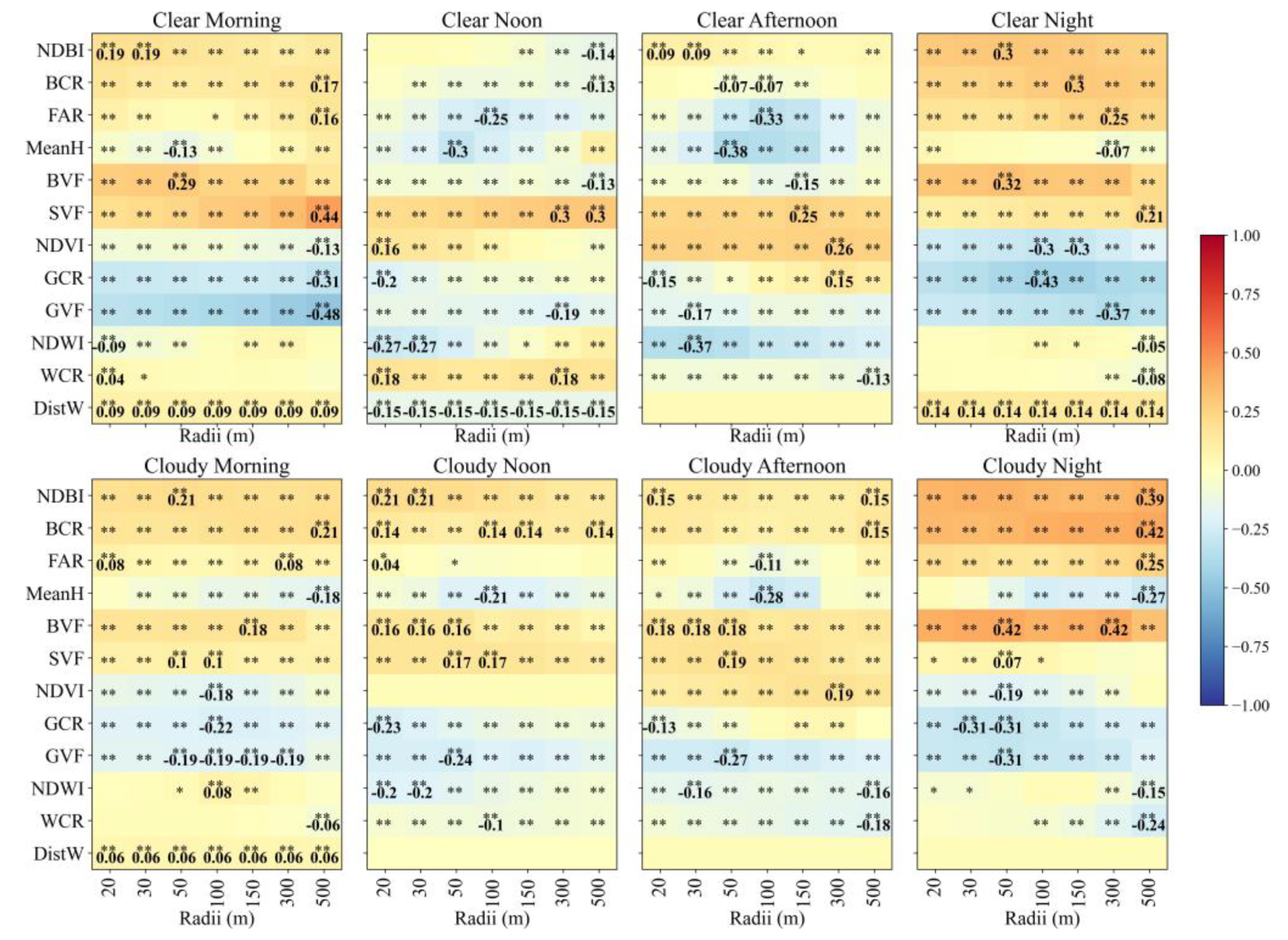
3.4. Influence of Land Cover and Morphological Parameters on the Microclimate

To determine the most appropriate buffer size for each morphological and land cover parameter based on its ability to capture the variations in ΔTa and ΔTw, the Pearson correlation coefficient was used to assess the relationship between the parameters and the temperature variables. As shown in Figure 10, the results vary depending on the time of day and sky conditions, with stronger correlations observed in the morning and cloudy nights. Overall, the correlations are much stronger on cloudy days than on clear days.
Specifically for the morphological parameters investigated, NDBI shows the strongest positive correlation with ΔTa on clear days, followed by BCR and the correlation coefficients of the two parameters are similar on cloudy days. FAR exhibits negative correlations with ΔTa during noon and afternoon (−0.12 and −0.16 in the 100 m radius, respectively) on clear days, however, they are positive on cloudy days, likely due to the solar radiation intercepted by high-rise buildings; this is confirmed by the negative correlations between MeanH and ΔTa during noon and afternoon (−0.27 and −0.37, respectively). On cloudy days, MeanH is still negatively correlated to ΔTa, obtaining higher values in the morning and evening (−0.32 and −0.33 in the 500 m radius, respectively) but lower values during noon and afternoon (−0.18 and −0.25 in the 100 m radius, respectively), suggesting the presence of other cooling mechanisms of high-rise buildings at a larger scale rather than the shading occurring on cloudy days; for instance, the extensive use of cooling surface materials in the central business district (route nine). BVF shows strong correlations with ΔTa in the morning and evening as well, but weak with correlation coefficients less than or equal to 0.1 during noon and afternoon on clear days. On the contrary, SVF is strongly correlated with ΔTa, with a coefficient of 0.32 at noon and 0.38 in the afternoon, suggesting that BVF and MeanH do not completely match due to GVF, especially in narrow street canyons. Concerning direct solar radiation from reaching the ground, SVF exhibits higher correlation coefficients during the day on clear days (from 0.32 to 0.45).
Vegetation-related parameters (NDVI, GCR, and GVF) are strongly and negatively correlated with ΔTa (−0.24~−0.56), except for NDVI during noon and afternoon. The correlations between NDVI and ΔTa are weak at noon (±0.06 on clear days and −0.12 on cloudy days) and even positive correlations in the afternoon occur (0.26 on clear days and 0.14 on cloudy days). The correlation between GCR and ΔTa in the evening is higher on cloudy days than on clear days (−0.54 and −0.32, respectively). GVF shows higher correlations on cloudy days except for morning and the diurnal variation on cloudy days is small (0.42~0.48), demonstrating the stable cooling effect of vegetation throughout the day on cloudy days.
The water-related parameters NDWI and WCR show negative correlations with ΔTa, except for WCR at noon on clear days (0.08 in the 20 m radius). The correlations between WCR and ΔTa on clear days are strongest in the afternoon (−0.35 in the 300 m radius) and remain significantly negative during the whole cloudy days, down to −0.29 at noon and up to −0.43 in the evening. NDWI shows higher correlations with ΔTa during noon and afternoon on clear days (−0.39 and −0.51, respectively) than on cloudy days (−0.27 and −0.33, respectively); on the other hand, the correlations are lower in the morning and evening on clear days (−0.16 and −0.1, respectively) than on cloudy days (−0.23 and −0.3, respectively). DistW significantly correlates with ΔTa, except for at noon on clear days, becoming higher on cloudy days (from 0.24 to 0.38).
Figure 11 shows the correlation between the land cover or morphological parameters and ΔTw. The correlation is generally weaker than that found between the parameters and ΔTa and generally stronger at night than during the daytime. During noon and afternoon on clear days, NDBI and BCR are no longer critical morphological parameters affecting Tw, but FAR and MeanH have strong negative correlations with ΔTw, over −0.25 and −0.3, respectively. SVF shows its peak correlation with ΔTw (0.44) during the morning of clear days, turning weaker (0.10) during the morning of cloudy days. BVF becomes the most significant morphological parameter in the evening, with correlations of 0.32 and 0.42 on clear days and cloudy days, respectively.
As for vegetation parameters, NDVI exhibits positive correlations with ΔTw during noon and afternoon up to 0.26, and negative in the morning and evening down to −0.19, which might relate to the increased moisture caused by evapotranspiration occurring under solar radiation. GCR and GVF have greater correlations in the morning and evening on clear days (up to −0.43 and −0.48, respectively) than on cloudy days (both up to −0.31). NDWI is negatively correlated with ΔTw during noon and afternoon under both sky conditions and stronger on clear days, obtaining a maximum of −0.37 in the afternoon of clear days. Interestingly, positive correlations between WCR and ΔTw reach 0.18 and are observed at noon on clear days. The highest correlation between WCR and ΔTw (−0.24) is in the evening of cloudy days. In addition, half of the correlations between DistW and ΔTw are insignificant and one of the significant correlations is negative.

4. Discussion

4.1. Impacts of GBI on Air Temperature with Different Urban Morphology

To study the cooling potential of GI and BI in different urban morphology, the medians of MeanH, GCR, GVF, and WCR (24.99 m, 0.4816, 0.3919, and 0.0323, respectively) are used to classify the traverse routes into 16 categories. GCRLGVFL and WCRL are the reference types representing the areas with the little help of GBI in cooling, divided into low-rise and high-rise areas. GCRLGVFH, GCRHGVFL, and GCRLGVFH mean abundant GI considered from the perspective of two and three-dimensional parameters and WCRH represents the areas adjacent to BI. By comparing the distributions of ΔTa in these categories, the respective cooling effects of GI and BI and their interactions can be obtained. The detailed street views shown in Figure 5a provide references for the following discussion.
Firstly, individual GI shows a stronger cooling effect of 0.27~0.76 °C in low-rise areas rather than 0.04~0.43 °C in high-rise areas (Figure 7a,b and Table 2). As shown in Figure 5a, when away from waterbodies, the low-rise street canyons are narrow and almost completely shaded by street trees and buildings, however, the proportion of shade in high-rise areas is not enough to reduce solar radiation from reaching the ground [47,48]. In low-rise areas, high GCR behaves with higher cooling potential during the morning and noon, and GVF is better during the afternoon and evening. Since solar radiation is moderate during the morning and noon, the evapotranspiration of GI is the primary cooling mechanism before the afternoon. Therefore, the amount of GI, that is, GCR, is the more critical greenery-related parameter. When the solar radiation intensifies in the afternoon, GI closes its stomata due to the excessive water loss and evapotranspiration decreases accordingly, and GVF becomes the dominating parameter on account of intercepting the solar radiation from reaching the pedestrian walkways. In the evening, thanks to the high GVF, less heat storage in the impervious material of buildings and pavements results in less heat emission, which leads to a lower ΔTa, even though slight UHI remains [49]. Evapotranspiration is important in cooling at night as well, however, it is a secondary cooling mechanism because the GI in low-rise areas is mostly street trees in old town districts rather than large lawns. In high-rise areas, high GVF reveals stronger cooling intensity rather than high GCR at each period. As detailed in Figure 5a, both the GCRLGVFH and GCRHGVFL in high-rise WCRL are characterized by street trees in the street canyons, indicating the differences between them refer to the differences in adjacent canopy coverage ratio and GVF, so the GVF among them is the key in cooling ambient air.
Individual BI has a stronger cooling effect in low-rise areas as well as GI, with the highest cooling intensity of 0.63 °C in the evening and the lowest 0.48 °C at noon, which are 0.46 °C and 0.17 °C, respectively, in high-rise areas (Figure 7 and Table 2). Since Figure 5a exhibits the openness of the low-rise areas, the possible reason would be that good ventilation induces higher wind speed, allowing the colder air near the water body to flow into the streets [50]. As the WCRH areas are generally accompanied by open urban morphology, in other words, low BCR, it can be regarded as LCZ 4: open high-rise and LCZ 5: open mid-rise, where LCZ represents the local climate zone (Figure 2b and Figure 4a) [26]. The “Mid-rise” here refers to the low-rise areas for the reason that low-rise buildings below the definition of 10 m are quite rare in Guangzhou. In contrast to these results, there is the lowest Ta in LCZ 4 in the afternoon in another study [51].
The integrated GBI sometimes inhibits cooling. In terms of GBI versus GI, in low-rise areas, during noon and afternoon, the addition of BI reduces the cooling intensity of GI, from 0.75 °C to 0.66 °C at noon and from 0.76 °C to 0.72 °C in the afternoon (Table 2). This interesting result is a supplement to the counterexamples of some reports in recent years [52,53]. On the other hand, in high-rise areas, the addition of BI helps the cooling of the air more effectively with sufficient GI, especially at noon and in the evening, with cooling intensity from 0.27 °C to 0.59 °C and from 0.18 °C to 0.62 °C, respectively.
Comparing GBI with BI, in WCRH areas, GCRLGVFH shows the highest median ΔTa in low-rise areas during the morning and noon and in high-rise areas in the morning and evening (Figure 7c,d). As shown in Figure 5a, GCRLGVFH in WCRH low-rise is the area with a double row of trees, however, the actual traverse route is near the northern bank of the river beside the outer row of trees on the island (route seven), which has high SVF and is directly exposed to the solar radiation during the day (Figure 4a and Figure 6). GCRLGVFH in high-rise areas may be poorly ventilated due to the proximity to the fairly close tall buildings and the canopy of the big trees, suggesting that trees in narrow streets can obstruct ventilation [47,49]. Notably, part of the GCRHGVFL in the WCRH high-rise type is the urban park (route ten), depicting the UHI in urban parks in the afternoon (Figure 6 and Figure 7c). It may be related to the size, geometry, and vegetation species layout (e.g., the dense trees around the park impede wind flow) of the park and the surrounding urban morphology, consistent with several studies [54,55]. In the evening in WCRH, the differences in ΔTa between different types of GI and the reference GCRLGVFL are up to 0.15 °C in low-rise areas and 0.16 °C in high-rise areas, revealing that the role of GI in further increasing the cooling intensity compared with individual BI.

4.2. Impacts of GBI on Wet Bulb Temperature with Different Urban Morphology

Since Tw is related to the heat transport between human bodies and the ambient atmosphere, it is necessary to consider the impact of GBI on Tw. Analogously, by comparing the distributions of ΔTw in various categories, the respective cooling effects of GI and BI and their interactions can be obtained. Overall, the medians of ΔTw in most of the types from noon to night are positive, especially during the afternoon and evening, suggesting that GBI alleviates but hardly reverses the positive ΔTw (Figure 9). As a result, humans inevitably feel slightly warmer in cities.
GI demonstrates its cooling potential on Tw in both low-rise and high-rise areas, where the former is higher and up to 0.55 °C in the evening while the latter is up to 0.16 °C in the afternoon (Table 3). In low-rise areas, the cooling intensity of high GCR for ΔTw is lower than that of high GVF during the day, which may be caused by the increased water vapor by evapotranspiration while Ta is relatively high (Figure 9a). In the evening, the cooling effect of GI is strongest in low-rise areas but weakest in high-rise areas. BI provides a 0.09~0.23 °C cooling intensity for ΔTw in low-rise and 0.00~0.15 °C in high-rise areas, where the peaks appear in the afternoon and the evening, respectively (Table 3). The cooling effect of BI on ΔTw is stronger during the afternoon and evening (Figure 9).
The integrated GBI in low-rise areas not only inhibits the cooling effect for ΔTw, but in GCRHGVFL even increases ΔTw up to 0.18 °C during the day (Figure 9a,c and Table 3). Comparing ΔTw in GCRHGVFH with different MeanH levels, the addition of BI reduces the cooling intensity in low-rise areas and enhances it in high-rise areas (Figure 9). Whether in low-rise or high-rise areas, high GVF seems useless in Tw cooling, which is reasonable since higher ΔTa is induced by the high SVF and poor ventilation (Figure 9c,d).
In general, the impacts of GBI on Tw with different urban morphology are similar to those on Ta. As shown in Figure 8, Tw is dominated by sky conditions rather than urban morphology and land cover, which is supported by the simultaneous higher Ta and RH during the transitional nighttime (Figure 2c).

4.3. Influence of GI and BI under Different Sky Conditions

The correlations between temperature (ΔTa) and different GI and BI parameters (GCR, GVF, NDVI, WCR, NDWI) are here compared between clear days and partially cloudy days. The results show that GCR and GVF have stronger negative correlations with ΔTa than NDVI for both clear days and partially cloudy days (Figure 10). Specifically, on clear days, the negative correlation coefficients between GCR and ΔTa are strongest in the morning (−0.51) and weakest at night (−0.32), while for partially cloudy days, the correlations are strongest for both morning (−0.51) and nighttime (−0.54). This may imply that the cooling effect from evapotranspiration of GI at night is higher on partially cloudy days than on clear days. In terms of GVF, the correlation coefficients are strongest in the morning (−0.56) and weakest at night (−0.24) for clear days, but are quite stable (−0.42~−0.48) on partially cloudy days. In summary, GI generally provides the strongest cooling effect on ΔTa in the morning. Moreover, the cooling effect of GI is generally higher on partially cloudy days than on clear days at night.
As two indicators of the BI, both NDWI and WCR are generally negatively correlated with ΔTa. Specifically, NDWI demonstrates the strongest correlation with ΔTa in the afternoon on both clear (−0.51) and partially cloudy days (−0.33). The correlations between NDWI and ΔTa are higher at noon and in the afternoon on clear days than on partially cloudy days, but lower in the morning and evening on clear days than on partially cloudy days. It should be noted that NDWI indirectly indicates GI due to its sensitivity to water content in vegetation and, thus, can have different effects from WCR on air temperature. On clear days, WCR has the strongest negative influence on ΔTa in the afternoon (−0.35) but even has a positive impact at noon (0.08). This can be attributed to the intense solar radiation reflecting off the waterbodies and heating the waterfront air, which diminishes in the afternoon (Figure 2c). On partially cloudy days, WCR is generally negatively correlated with ΔTa throughout the day. In addition, DistW is found to be positively related to ΔTa, with the strongest correlations observed in the morning under both sky conditions and stronger correlations on partially cloudy days at any time. When the analysis object becomes ΔTw, we find positive correlations between NDVI and ΔTw at noon on clear days (0.16) and in the afternoon on both clear (0.26) and cloudy days (0.19), which can be attributed to the process of evapotranspiration from the greenery that increases the water vapor in the air and further increases the humidity-related variable ΔTw. In the afternoon, correlations albeit negative, occur in small radii from 20 m to 50 m; positive correlations between GCR and ΔTw are observed in larger radii, suggesting that GI could induce warming ΔTw at the local scale. GCR has the most direct cooling effect on ΔTw on clear evenings, which could be explained by stronger evapotranspiration on clear nights than on partially cloudy nights, which is related to less residual water in GI with higher ambient temperature. GVF exhibits the largest negative correlation with ΔTw on clear mornings (−0.48), followed by the correlation in the evening (−0.37), indicating that the tree canopy may play a role in slowing the exchange of cooling air trapped in the street canyons at night with the air heated by solar radiation in the morning. As dew is common the next morning on a clear night, the moisture content of the ambient air near greenery in the morning tends to be oversaturated. Therefore, it is low Ta and high humidity that leads to high Tw.
NDWI and WCR do not show clear relationships with ΔTw in the morning and on clear evenings, suggesting that BI may not have a strong cooling effect on ΔTw during those times. Furthermore, positive correlations are found on clear noontimes between WCR and ΔTw (0.18), but these turn into negative correlations on clear afternoons (−0.13), possibly due to high evaporation rates from waterbodies under the most direct and strongest solar radiation at noon, increasing water vapor at high Ta and leading to higher ΔTw (Figure 2c and Figure 8). On partially cloudy days, the strongest correlation between WCR and ΔTw appears in the evening (−0.24), however, it is insignificant in the radii smaller than 100 m. Therefore, the correlation might be related to the distinct waterfront urban morphology and GI rather than BI itself.

4.4. Limitations and Future Studies

In this study, we present a methodological framework for investigating the diurnal variations in the impact of GBI on the thermal environment along pedestrian walkways by integrating multiple data sources. Limitations include the limited time frame and location of the measurements, as well as the use of mobile measurement devices, which may not provide as accurate or comprehensive data as stationary measurement devices. We further acknowledge the importance of conducting measurements in various seasons, including summer. However, GBI exhibits distinct but less frequently studied thermal characteristics in winter that can be different from other seasons. Conducting the experiment in winter can also complement the existing understanding of the impact of GBI on the thermal environment with different weather patterns. Additionally, the study can be biased towards cycling routes and does not include other modes of pedestrian pathways.
Future studies could expand on the findings by conducting measurements in different pedestrian locations and at different times of the year to provide a more comprehensive understanding of the thermal environment on pedestrian and cycling routes. Additionally, more advanced measurement devices, such as Lidar and video streaming, may be necessary to provide more accurate and comprehensive data. The study could also be expanded to include a wider range of urban forms and densities and to evaluate human thermal comfort indices, such as UTCI and PET, to provide more comprehensive information on urban planning and design.

5. Conclusions

This study investigated the impacts of urban GBI on the outdoor thermal environment along pedestrian walkways by conducting a mobile measurement campaign in Guangzhou (China) during winter. We investigated the heterogeneity of Ta and Tw and their correlations with urban morphological and land cover parameters (six building-related, three vegetation-related, and three water-related). Results show that both GI and BI show a stronger cooling effect on Ta and Tw in low-rise areas than in high-rise areas. Specifically, GI can lower Ta by up to 0.76 °C in low-rise and 0.43 °C in high-rise areas in the afternoon and Tw by up to 0.55 °C in low-rise areas (evening) and 0.16 °C in high-rise areas (afternoon). BI can lower Ta by up to 0.63 °C and 0.46 °C in the evening in low-rise and high-rise areas, respectively, and can lower Tw by up to 0.23 °C in low-rise areas (afternoon) and 0.15 °C in high-rise areas (evening). Compared to individual GI or BI, integrating the two results in enhanced cooling for both Ta and Tw in high-rise areas, but weakens Tw cooling during noon and afternoon in low-rise areas. Moreover, different parameters, such as GCR and GVF, play a dominant role in cooling depending on the proximity to BI and the time of day. Away from BI, during the morning and noon in low-rise areas, the dominant GI parameter contributing to cooling is GCR, while it is GVF in other cases. Adjacent to BI, the dominant GI parameter that accounts for cooling is always GCR.
On clear days, correlation analyses show that GI (NDVI, GCR, and GVF) exhibit the strongest negative correlations with Ta in the morning, while water-related parameters (NDWI and WCR) have the strongest correlation with Ta cooling in the afternoon. On cloudy days, GI has strong correlations with Ta cooling in both morning and evening and the correlations between BI and Ta are similar at different periods. Different from Ta, the correlations between GI and Tw are prominent in the morning and evening on clear days, while NDWI and WCR show the strongest correlation with Tw cooling in the afternoon (−0.37 and −0.13, respectively). On cloudy days, the strongest correlations between GI and Tw cooling all appear in the evening and the correlations between BI and Ta are weak in the morning.
This study provides insights into the thermal regulation effect of GBI on pedestrian walkways and is useful for designing and planning climate-adaptive strategies. While urban GBI helps to alleviate the outdoor thermal environment on pedestrian walkways by reducing Ta and Tw, the cooling effect of GI–BI integration may not be as effective as that of individual GI in some built-up environments, highlighting the cautious planning and design of GBI. Additionally, the cooling effect of GBI varies with the time of day and sky conditions.

Author Contributions

Conceptualization, L.Z. and H.P.; methodology, L.Z. and H.P.; software, L.Z. and H.P.; validation, H.P. and Y.L.; formal analysis, H.P.; investigation, H.P. and L.Z.; resources, J.H. (Jian Hang), L.Z., Y.S., R.B. and J.H. (Jiajia Hua); data curation, H.P., L.Z. and Y.L.; writing—original draft preparation, H.P. and L.Z.; writing—review and editing, H.P., L.Z., R.B., Y.L., Y.S., J.H. (Jian Hang), X.Z., J.H. (Jiajia Hua), B.Z. and Z.G.; visualization, H.P., L.Z. and Y.L.; supervision, J.H. (Jian Hang) and L.Z.; project administration, J.H. (Jian Hang); funding acquisition, J.H. (Jian Hang) and L.Z. All authors have read and agreed to the published version of the manuscript.

Funding

This research was funded by the National Natural Science Foundation of China (nos. 42105070 and 42175095), the Guangdong Basic and Applied Basic Research Foundation (no. 2020A1515110278), and the Innovation Group Project of Southern Marine Science and Engineering Guangdong Laboratory (no. 311020001).

Institutional Review Board Statement

Not applicable.

Informed Consent Statement

Not applicable.

Data Availability Statement

Not applicable.

Acknowledgments

The authors would like to thank Lin Liu, Zhonghua Wu, Shiying Lan, Jianwen Gao, Yushuang Zhu, Yuhong Cai, Shuzhang Yang, Zhenxi Liang, Yubin Liao, Jianbin Mo, and Yongkang Mai of the School of Civil and Transportation Engineering, Guangdong University of Technology for their hard work during the field survey.

Conflicts of Interest

The authors declare no conflict of interest. The funders had no role in the design of the study; in the collection, analyses, or interpretation of data; in the writing of the manuscript; or in the decision to publish the results.

Nomenclature

BCRBuilding coverage ratio
BIBlue infrastructure
BVFBuilding-view factor
CUHICanopy urban heat island
DistWDistance to water bodies
FARFloor area ratio
GBIGreen and blue infrastructure
GCRGreenery coverage ratio
GIGreen infrastructure
GISGeographic information system
GVFGreenery-view factor
LCZLocal climate zone
LSTLand surface temperature
LURLand-use regression
MeanHMean height of buildings
MIRMid-infrared spectral range
NDBINormalized difference built-up index
NDVINormalized difference vegetation index
NDWINormalized difference water index
NIRNear-infrared spectral range
PCEPark cooling effect
RHRelative humidity
PCIPark cooling island
SUHISurface urban heat island
SVFSky-view factor
SWIRShortwave infrared spectral range
TaAir temperature
TwWet-bulb temperature
UCIUrban cooling island
UHIUrban heat island
WCRWater coverage ratio

References

  1. Sun, Z.; Chen, C.; Yan, M.; Shi, W.; Wang, J.; Ban, J.; Sun, Q.; He, M.Z.; Li, T. Heat Wave Characteristics, Mortality and Effect Modification by Temperature Zones: A Time-Series Study in 130 Counties of China. Int. J. Epidemiol. 2020, 49, 1813–1822. [Google Scholar] [CrossRef] [PubMed]
  2. Yang, J.; Yin, P.; Sun, J.; Wang, B.; Zhou, M.; Li, M.; Tong, S.; Meng, B.; Guo, Y.; Liu, Q. Heatwave and Mortality in 31 Major Chinese Cities: Definition, Vulnerability and Implications. Sci. Total Environ. 2019, 649, 695–702. [Google Scholar] [CrossRef] [PubMed]
  3. Burkart, K.; Meier, F.; Schneider, A.; Breitner, S.; Canário, P.; Alcoforado, M.J.; Scherer, D.; Endlicher, W. Modification of Heat-Related Mortality in an Elderly Urban Population by Vegetation (Urban Green) and Proximity to Water (Urban Blue): Evidence from Lisbon, Portugal. Environ. Health Perspect. 2016, 124, 927–934. [Google Scholar] [CrossRef] [PubMed] [Green Version]
  4. Chen, L.; Ng, E.; An, X.; Ren, C.; Lee, M.; Wang, U.; He, Z. Sky View Factor Analysis of Street Canyons and Its Implications for Daytime Intra-Urban Air Temperature Differentials in High-Rise, High-Density Urban Areas of Hong Kong: A GIS-Based Simulation Approach. Int. J. Climatol. 2012, 32, 121–136. [Google Scholar] [CrossRef]
  5. He, C.; Zhou, L.; Yao, Y.; Ma, W.; Kinney, P.L. Estimating Spatial Effects of Anthropogenic Heat Emissions upon the Urban Thermal Environment in an Urban Agglomeration Area in East China. Sustain. Cities Soc. 2020, 57, 102046. [Google Scholar] [CrossRef]
  6. Jiang, Z.; Cheng, H.; Zhang, P.; Kang, T. Influence of Urban Morphological Parameters on the Distribution and Diffusion of Air Pollutants: A Case Study in China. J. Environ. Sci. 2021, 105, 163–172. [Google Scholar] [CrossRef]
  7. Yuan, C.; Zhu, R.; Tong, S.; Mei, S.; Zhu, W. Impact of Anthropogenic Heat from Air-Conditioning on Air Temperature of Naturally Ventilated Apartments at High-Density Tropical Cities. Energy Build. 2022, 268, 112171. [Google Scholar] [CrossRef]
  8. Zhou, L.; Hu, F.; Wang, B.; Wei, C.; Sun, D.; Wang, S. Relationship between Urban Landscape Structure and Land Surface Temperature: Spatial Hierarchy and Interaction Effects. Sustain. Cities Soc. 2022, 80, 103795. [Google Scholar] [CrossRef]
  9. Gunawardena, K.R.; Wells, M.J.; Kershaw, T. Utilising Green and Bluespace to Mitigate Urban Heat Island Intensity. Sci. Total Environ. 2017, 584–585, 1040–1055. [Google Scholar] [CrossRef]
  10. Saaroni, H.; Amorim, J.H.; Hiemstra, J.A.; Pearlmutter, D. Urban Green Infrastructure as a Tool for Urban Heat Mitigation: Survey of Research Methodologies and Findings across Different Climatic Regions. Urban Clim. 2018, 24, 94–110. [Google Scholar] [CrossRef]
  11. Geng, X.; Yu, Z.; Zhang, D.; Li, C.; Yuan, Y.; Wang, X. The Influence of Local Background Climate on the Dominant Factors and Threshold-Size of the Cooling Effect of Urban Parks. Sci. Total Environ. 2022, 823, 153806. [Google Scholar] [CrossRef]
  12. Lu, J.; Li, Q.; Zeng, L.; Chen, J.; Liu, G.; Li, Y.; Li, W.; Huang, K. A Micro-Climatic Study on Cooling Effect of an Urban Park in a Hot and Humid Climate. Sustain. Cities Soc. 2017, 32, 513–522. [Google Scholar] [CrossRef]
  13. Park, J.; Kim, J.-H.; Lee, D.K.; Park, C.Y.; Jeong, S.G. The Influence of Small Green Space Type and Structure at the Street Level on Urban Heat Island Mitigation. Urban For. Urban Green. 2017, 21, 203–212. [Google Scholar] [CrossRef]
  14. Bowler, D.E.; Buyung-Ali, L.; Knight, T.M.; Pullin, A.S. Urban Greening to Cool Towns and Cities: A Systematic Review of the Empirical Evidence. Landsc. Urban Plan. 2010, 97, 147–155. [Google Scholar] [CrossRef]
  15. Skelhorn, C.; Lindley, S.; Levermore, G. The Impact of Vegetation Types on Air and Surface Temperatures in a Temperate City: A Fine Scale Assessment in Manchester, UK. Landsc. Urban Plan. 2014, 121, 129–140. [Google Scholar] [CrossRef]
  16. Vaz Monteiro, M.; Doick, K.J.; Handley, P.; Peace, A. The Impact of Greenspace Size on the Extent of Local Nocturnal Air Temperature Cooling in London. Urban For. Urban Green. 2016, 16, 160–169. [Google Scholar] [CrossRef]
  17. Lemoine-Rodríguez, R.; Inostroza, L.; Falfán, I.; MacGregor-Fors, I. Too Hot to Handle? On the Cooling Capacity of Urban Green Spaces in a Neotropical Mexican City. Urban For. Urban Green. 2022, 74, 127633. [Google Scholar] [CrossRef]
  18. Yu, Z.; Guo, X.; Jørgensen, G.; Vejre, H. How Can Urban Green Spaces Be Planned for Climate Adaptation in Subtropical Cities? Ecol. Indic. 2017, 82, 152–162. [Google Scholar] [CrossRef]
  19. He, C.; Zhou, L.; Yao, Y.; Ma, W.; Kinney, P.L. Cooling Effect of Urban Trees and Its Spatiotemporal Characteristics: A Comparative Study. Build. Environ. 2021, 204, 108103. [Google Scholar] [CrossRef]
  20. Doick, K.J.; Peace, A.; Hutchings, T.R. The Role of One Large Greenspace in Mitigating London’s Nocturnal Urban Heat Island. Sci. Total Environ. 2014, 493, 662–671. [Google Scholar] [CrossRef]
  21. Hathway, E.A.; Sharples, S. The Interaction of Rivers and Urban Form in Mitigating the Urban Heat Island Effect: A UK Case Study. Build. Environ. 2012, 58, 14–22. [Google Scholar] [CrossRef] [Green Version]
  22. Theeuwes, N.E.; Solcerová, A.; Steeneveld, G.J. Modeling the Influence of Open Water Surfaces on the Summertime Temperature and Thermal Comfort in the City. J. Geophys. Res. Atmos. 2013, 118, 8881–8896. [Google Scholar] [CrossRef] [Green Version]
  23. Sun, R.; Chen, L. How Can Urban Water Bodies Be Designed for Climate Adaptation? Landsc. Urban Plan. 2012, 105, 27–33. [Google Scholar] [CrossRef]
  24. Steeneveld, G.J.; Koopmans, S.; Heusinkveld, B.G.; Theeuwes, N.E. Refreshing the Role of Open Water Surfaces on Mitigating the Maximum Urban Heat Island Effect. Landsc. Urban Plan. 2014, 121, 92–96. [Google Scholar] [CrossRef]
  25. Du, H.; Cai, W.; Xu, Y.; Wang, Z.; Wang, Y.; Cai, Y. Quantifying the Cool Island Effects of Urban Green Spaces Using Remote Sensing Data. Urban For. Urban Green. 2017, 27, 24–31. [Google Scholar] [CrossRef]
  26. Stewart, I.D.; Oke, T.R. Local Climate Zones for Urban Temperature Studies. Bull. Am. Meteorol. Soc. 2012, 93, 1879–1900. [Google Scholar] [CrossRef]
  27. Pigliautile, I.; Pisello, A.L. A New Wearable Monitoring System for Investigating Pedestrians’ Environmental Conditions: Development of the Experimental Tool and Start-up Findings. Sci. Total Environ. 2018, 630, 690–706. [Google Scholar] [CrossRef] [PubMed]
  28. Cao, C.; Yang, Y.; Lu, Y.; Schultze, N.; Gu, P.; Zhou, Q.; Xu, J.; Lee, X. Performance Evaluation of a Smart Mobile Air Temperature and Humidity Sensor for Characterizing Intra-City Thermal Environment. J. Atmos. Ocean. Technol. 2020, 37, 1891–1905. [Google Scholar] [CrossRef]
  29. Ulpiani, G. On the Linkage between Urban Heat Island and Urban Pollution Island: Three-Decade Literature Review towards a Conceptual Framework. Sci. Total Environ. 2021, 751, 141727. [Google Scholar] [CrossRef]
  30. Kousis, I.; Manni, M.; Pisello, A.L. Environmental Mobile Monitoring of Urban Microclimates: A Review. Renew. Sustain. Energy Rev. 2022, 169, 112847. [Google Scholar] [CrossRef]
  31. Cassano, J.J. Weather Bike: A Bicycle-Based Weather Station for Observing Local Temperature Variations. Bull. Am. Meteorol. Soc. 2014, 95, 205–209. [Google Scholar] [CrossRef]
  32. Climate Bulletin of Guangzhou. Available online: http://www.tqyb.com.cn/gz/climaticprediction/bulletin/2022-03-10/9924.html (accessed on 1 June 2023).
  33. Shi, Y.; Xiang, Y.; Zhang, Y. Urban Design Factors Influencing Surface Urban Heat Island in the High-Density City of Guangzhou Based on the Local Climate Zone. Sensors 2019, 19, 3459. [Google Scholar] [CrossRef] [PubMed] [Green Version]
  34. Baidu Map Panorama. Available online: https://map.baidu.com/ (accessed on 3 June 2023).
  35. Shi, Y.; Lau, K.K.-L.; Ng, E. Developing Street-Level PM2.5 and PM10 Land Use Regression Models in High-Density Hong Kong with Urban Morphological Factors. Environ. Sci. Technol. 2016, 50, 8178–8187. [Google Scholar] [CrossRef] [PubMed]
  36. Qi, M.; Hankey, S. Using Street View Imagery to Predict Street-Level Particulate Air Pollution. Environ. Sci. Technol. 2021, 55, 2695–2704. [Google Scholar] [CrossRef]
  37. Zeng, L.; Hang, J.; Wang, X.; Shao, M. Influence of Urban Spatial and Socioeconomic Parameters on PM2.5 at Subdistrict Level: A Land Use Regression Study in Shenzhen, China. J. Environ. Sci. 2022, 114, 485–502. [Google Scholar] [CrossRef]
  38. Gong, F.-Y.; Zeng, Z.-C.; Ng, E.; Norford, L.K. Spatiotemporal Patterns of Street-Level Solar Radiation Estimated Using Google Street View in a High-Density Urban Environment. Build. Environ. 2019, 148, 547–566. [Google Scholar] [CrossRef]
  39. Liang, J.; Gong, J.; Sun, J.; Zhou, J.; Li, W.; Li, Y.; Liu, J.; Shen, S. Automatic Sky View Factor Estimation from Street View Photographs—A Big Data Approach. Remote Sens. 2017, 9, 411. [Google Scholar] [CrossRef] [Green Version]
  40. Brown, M.J.; Grimmond, S.; Ratti, C. Comparison of Methodologies for Computing Sky View Factor in Urban Environments. In Proceedings of the 2001 International Symposium on Environmental Hydraulics, Tempe, AZ, USA, 5–8 December 2001; p. 6. [Google Scholar]
  41. Johnson, G.T.; Watson, I.D. The Determination of View-Factors in Urban Canyons. J. Appl. Meteorol. Clim. 1984, 23, 329–335. [Google Scholar] [CrossRef]
  42. Watson, I.D.; Johnson, G.T. Graphical Estimation of Sky View-Factors in Urban Environments. J. Climatol. 1987, 7, 193–197. [Google Scholar] [CrossRef]
  43. Zeng, L.; Lu, J.; Li, W.; Li, Y. A Fast Approach for Large-Scale Sky View Factor Estimation Using Street View Images. Build. Environ. 2018, 135, 74–84. [Google Scholar] [CrossRef]
  44. Sherwood, S.C.; Huber, M. An Adaptability Limit to Climate Change Due to Heat Stress. Proc. Natl. Acad. Sci. USA 2010, 107, 9552–9555. [Google Scholar] [CrossRef] [Green Version]
  45. World Meteorological Organization. Guide to Meteorological Instruments and Methods of Observation: Preliminary Seventh Edition; Secretariat of the World Meteorological Organization: Geneva, Switzerland, 2006. [Google Scholar]
  46. Moratiel, R.; Soriano, B.; Centeno, A.; Spano, D.; Snyder, R.L. Wet-Bulb, Dew Point, and Air Temperature Trends in Spain. Theor. Appl. Climatol. 2017, 130, 419–434. [Google Scholar] [CrossRef]
  47. Chen, T.; Pan, H.; Lu, M.; Hang, J.; Lam, C.K.C.; Yuan, C.; Pearlmutter, D. Effects of Tree Plantings and Aspect Ratios on Pedestrian Visual and Thermal Comfort Using Scaled Outdoor Experiments. Sci. Total Environ. 2021, 801, 149527. [Google Scholar] [CrossRef]
  48. Jin, H.; Cui, P.; Wong, N.; Ignatius, M. Assessing the Effects of Urban Morphology Parameters on Microclimate in Singapore to Control the Urban Heat Island Effect. Sustainability 2018, 10, 206. [Google Scholar] [CrossRef] [Green Version]
  49. Probst, N.; Bach, P.M.; Cook, L.M.; Maurer, M.; Leitão, J.P. Blue Green Systems for Urban Heat Mitigation: Mechanisms, Effectiveness and Research Directions. Blue-Green Syst. 2022, 4, 348–376. [Google Scholar] [CrossRef]
  50. Park, C.Y.; Lee, D.K.; Asawa, T.; Murakami, A.; Kim, H.G.; Lee, M.K.; Lee, H.S. Influence of Urban Form on the Cooling Effect of a Small Urban River. Landsc. Urban Plan. 2019, 183, 26–35. [Google Scholar] [CrossRef]
  51. Jiang, L.; Liu, S.; Liu, L.; Liu, C. Revealing the Spatiotemporal Characteristics and Drivers of the Block-Scale Thermal Environment near a Large River: Evidences from Shanghai, China. Build. Environ. 2022, 226, 109728. [Google Scholar] [CrossRef]
  52. Hou, J.; Mao, H.; Li, J.; Sun, S. Spatial Simulation of the Ecological Processes of Stormwater for Sponge Cities. J. Environ. Manag. 2019, 232, 574–583. [Google Scholar] [CrossRef] [PubMed]
  53. Jacobs, C.; Klok, L.; Bruse, M.; Cortesão, J.; Lenzholzer, S.; Kluck, J. Are Urban Water Bodies Really Cooling? Urban Clim. 2020, 32, 100607. [Google Scholar] [CrossRef]
  54. Cao, X.; Onishi, A.; Chen, J.; Imura, H. Quantifying the Cool Island Intensity of Urban Parks Using ASTER and IKONOS Data. Landsc. Urban Plan. 2010, 96, 224–231. [Google Scholar] [CrossRef]
  55. Motazedian, A.; Coutts, A.M.; Tapper, N.J. The Microclimatic Interaction of a Small Urban Park in Central Melbourne with Its Surrounding Urban Environment during Heat Events. Urban For. Urban Green. 2020, 52, 126688. [Google Scholar] [CrossRef]
Figure 1. The schematic framework for this study, in which red boxes represent the acquisition of air temperature and wet-bulb temperature, the blue boxes represent the acquisition of land cover and morphological parameters, and the purple boxes represent the perspectives of analyses.
Atmosphere 14 01037 g001
Figure 2. (a) Locations of the traverse campaign and background weather station; (b) land cover classification (derived from the geographic information system (GIS) landcover database of the central urbanized area of Guangzhou provided by Shi et al. [33]) of the study area and LCZ types of the traverse routes with the corresponding street views (screen-captured from Baidu Map [34], which is an open-access e-map service in China); (c) background meteorological conditions, including air temperature, humidity, wind, and shortwave solar radiation data from a nearby weather station.
Atmosphere 14 01037 g002
Figure 3. A circular buffer of an aggregation point.
Atmosphere 14 01037 g003
Figure 4. (a) Spatial distributions within a 150 m radius and (b) frequency distributions of the urban morphological and land cover parameters along the mobile measurement routes examined in this study in optimal radius.
Atmosphere 14 01037 g004aAtmosphere 14 01037 g004b
Figure 5. (a) Baidu street-view images (screen-captured from Baidu Map [34]) with various types of traverse routes classified by MeanH, GCR, GVF, and WCR; (b) spatial variations of BCR, NDBI, WCR, and NDWI on the various types of traverse routes classified by MeanH, GCR, GVF, and WCR. The subscript “L” indicates the data lower than the median and the subscript “H” indicates the data higher than the median. The boxes represent the 25th to the 75th percentile (IQR = interquartile range = quartile 3–quartile 1) and the upper and lower whiskers correspond to the upper and lower limits, respectively. The lines inside the boxes are the median values.
Atmosphere 14 01037 g005aAtmosphere 14 01037 g005b
Figure 6. Spatial distribution of ΔTa along the traverse routes during the morning, noon, afternoon, and night measurement periods.
Atmosphere 14 01037 g006
Figure 7. Boxplots of the ΔTa distribution in the various types of traverse routes classified by MeanH, GCR, GVF, and WCR: (a) types of WCRL, Low-rise; (b) types of WCRL, High-rise; (c) types of WCRH, Low-rise; (d) types of WCRH, High-rise. The subscript “L” means the data lower than the median and the subscript “H” means the data higher than the median. The boxes represent the 25th to the 75th percentile (IQR = interquartile range = quartile 3–quartile 1) and the upper and lower whiskers correspond to the upper and lower limits, respectively. The lines inside the boxes are the median values.
Atmosphere 14 01037 g007
Figure 8. Spatial distribution of ΔTw along the traverse routes during the morning, noon, afternoon, and evening measurement periods.
Atmosphere 14 01037 g008
Figure 9. Boxplots of the ΔTw distribution in the various types of traverse routes classified by MeanH, GCR, GVF, and WCR: (a) types of WCRL, Low-rise; (b) types of WCRL, High-rise; (c) types of WCRH, Low-rise; (d) types of WCRH, High-rise. The subscript “L” indicates the data lower than the median and the subscript “H” indicates the data higher than the median. The boxes represent the 25th to the 75th percentile (IQR = interquartile range = quartile 3–quartile 1) and the upper and lower whiskers correspond to the upper and lower limits, respectively. The lines inside the boxes are the median values.
Atmosphere 14 01037 g009
Figure 10. Correlation coefficients between ΔTa and multiple morphological and land cover parameters; correlation coefficients with significance level test of p ≥ 0.05 are marked with blank space; ** significant correlation at the 0.01 level; * significant correlation at the 0.05 level.
Atmosphere 14 01037 g010
Figure 11. Correlation coefficients between ΔTw and multiple morphological and land cover parameters; correlation coefficients with significance level test of p ≥ 0.05 are marked with blank space; ** significant correlation at the 0.01 level; * significant correlation at the 0.05 level.
Atmosphere 14 01037 g011
Table 1. Specifications of the instruments.
ParametersInstrumentsResponse TimeAccuracyRange
TaSmart-T 1~8 s−0.01~0.23 °C−40~60 °C
RH−1.4~1.9%10~90%
TastationIRGASON/±0.17 °C−80~60 °C
RHstation±1.0% (0~90%) or
±1.7% (90~100%)
0~100%
1 Smart-T is a Ta and RH sensor cooperatively developed and produced by Yale-NUIST Center on Atmospheric Environment, Nanjing University of Information Science & Technology, Nanjing 210044, China, and Jiangsu Radio Scientific Institute Corporation, Wuxi 214072, China.
Table 2. ΔTa median differences between various types and the reference type.
WCRMeanHGCR, GVFMorningNoonAfternoonEvening
LowLow-riseLow, low/ 1/ 1/ 1/ 1
Low, high−0.52−0.45−0.50−0.53
High, low−0.61−0.46−0.27−0.42
High, high−0.63−0.75−0.76−0.69
High-riseLow, low/ 2/ 2/ 2/ 2
Low, high−0.13−0.20−0.28−0.13
High, low−0.04−0.20−0.17−0.07
High, high−0.14−0.27−0.43−0.18
HighLow-riseLow, low−0.53−0.48−0.53−0.63
Low, high−0.44−0.35−0.34−0.68
High, low−0.66−0.49−0.29−0.72
High, high−0.73−0.66−0.72−0.78
High-riseLow, low−0.29−0.17−0.35−0.46
Low, high−0.21−0.24−0.39−0.36
High, low−0.27−0.59−0.69−0.62
High, high−0.35−0.58−0.64−0.54
1 WCRL, low-rise, GCRLGVFL was chosen as the reference type for any other low-rise cases. 2 WCRL, high-rise, GCRLGVFL was chosen as the reference type for any other high-rise cases.
Table 3. ΔTw median differences between various types and the reference type.
WCRMeanHGCR, GVFMorningNoonAfternoonEvening
LowLow-riseLow, low/ 1/ 1/ 1/ 1
Low, high−0.37−0.30−0.32−0.32
High, low−0.19−0.170.03−0.38
High, high−0.36−0.33−0.38−0.55
High-riseLow, low/ 2/ 2/ 2/ 2
Low, high−0.09−0.14−0.12−0.07
High, low−0.10−0.12−0.08−0.03
High, high−0.03−0.15−0.16−0.09
HighLow-riseLow, low−0.09−0.10−0.23−0.17
Low, high0.010.08−0.02−0.18
High, low−0.080.000.18−0.31
High, high−0.29−0.16−0.18−0.29
High-riseLow, low−0.060.00−0.14−0.15
Low, high−0.11−0.03−0.14−0.19
High, low−0.09−0.23−0.29−0.18
High, high−0.15−0.20−0.26−0.15
1 WCRL, low-rise, GCRLGVFL was chosen as the reference type for any other low-rise cases. 2 WCRL, high-rise, GCRLGVFL was chosen as the reference type for any other high-rise cases.
Disclaimer/Publisher’s Note: The statements, opinions and data contained in all publications are solely those of the individual author(s) and contributor(s) and not of MDPI and/or the editor(s). MDPI and/or the editor(s) disclaim responsibility for any injury to people or property resulting from any ideas, methods, instructions or products referred to in the content.

