1. Introduction
Ionospheric irregularities in the nighttime equatorial region are primarily equatorial spread F (ESF) irregularities caused by the generalized Rayleigh–Taylor instability [
1]. The Rayleigh–Taylor instability is excited in the bottomside F region, and evolves nonlinearly into topside plasma bubbles. Plasma density irregularities associated with plasma bubbles occur over several orders of magnitude in spatial scale, from hundreds of kilometers to less than 0.1 m. Statistical patterns of occurrence of ESF irregularities have been derived based on satellite measurements [
2]. The ESF occurrence probability depends on longitude and season, and is high in the African–South American sector and relatively low in the Asian–Pacific sector. ESF occurs more frequently in equinoctial months, which may be controlled by the alignment between the geomagnetic field lines and the sunset terminator [
3]. Refs. [
4,
5] found that the global distribution of the vertical plasma drift in the post-sunset sector (the pre-reversal enhancement, PRE) is very similar to that of the ESF occurrence, indicating that the enhanced PRE of the vertical plasma drift is the primary factor that controls the generation of equatorial plasma bubbles and ESF.
Ionospheric irregularities cause the scintillation of trans-ionospheric radio signals over a wide range of frequencies, from VHF/UHF to the L band. Refs. [
6,
7] derived global variations of amplitude scintillation fades. Severe scintillations often occur at low latitudes in the evening sector, especially during solar maximum periods. The scintillation effect on radio waves is stronger at lower frequencies, such as VHF [
8,
9,
10]. Ref. [
11] compared the occurrence of ESF irregularities with the scintillation S4 index during low and moderate solar activity and identified good agreement in the global distribution of the two phenomena. Refs. [
12,
13] developed a three-dimensional model for the plasma plumes caused by interchange instabilities in the low-latitude ionosphere to describe the structure and extent of the radio scintillation generated by turbulence in and around the plumes. These statistical patterns or numerical models provide a reasonable description of the global morphology of ionospheric irregularities and scintillation.
On the other hand, the global models/patterns may not be able to provide all features of scintillation at a specific location. In the Pacific longitude sector, the statistical patterns [
2,
4] show that the ESF occurrence probability gradually and continuously increases from March to August. An early observational study [
14] found that VHF/UHF scintillation occurrence over Kwajalein was high in May and July but low in June, which is inconsistent with the statistical ESF patterns. ESF irregularities are the primary cause of radio scintillation, and scintillation can lead to the degradation and disruption of communications and navigation. Identifying scintillation characteristics at specific locations is an important task for the space community.
In this study, we focus on scintillation activity over Kwajalein Atoll in the Marshall Islands, making use of multiple instruments that were installed to measure various ionospheric parameters and scintillation. We processed VHF scintillation data received at Kwajalein during moderate solar activity in 2012, examining the variations of VHF scintillation with month and local time and the features that are different from, or not reported in, previous observations. We also compared VHF scintillation data with ionospheric irregularities and ion drifts observed with the Communication/Navigation Outage Forecasting System (C/NOFS) satellite. The objectives of this study are to reveal the occurrence characteristics of VHF scintillation at Kwajalein and to identify the mechanisms responsible for the variations of scintillation in the Pacific region.
2. Observations of VHF Scintillation at Kwajalein
Kwajalein is located at 8.72° N, 167.73° E (3.79° magnetic latitude), an ideal location for studying equatorial scintillation. The signals used in this study were transmitted from a geostationary satellite in the VHF range (about 240 MHz) and received at Kwajalein throughout the entire year of 2012. The data were continuously recorded, without any significant gap. For scintillation studies, we analyzed the data between 08:00 and 20:00 UT, corresponding to 19:00–07:00 LT (LT = UT + 11 h), because equatorial ionospheric scintillation is caused primarily by ESF irregularities associated with plasma bubbles, and occurs exclusively during nighttime.
Figure 1 presents examples of VHF scintillation over two nights in 2012.
Figure 1a,b show the VHF power and the S4 index observed on 19 April, 2012, respectively. The black curve in
Figure 1a represents the received VHF signals and the green line represents the undisturbed signal level. It is clear that very large fluctuations started to occur at 09:10 UT, as denoted by the vertical dotted line.
Figure 1b shows the S4 index calculated from VHF amplitude fluctuations. The strength of amplitude scintillations is quantified by the S4 index [
15]. The S4 index is defined as the ratio of the standard deviation of the signal power to the mean signal power computed over a period of time (typically 1 min),
where the brackets indicate ensemble averaging. In our case, the VHF data were recorded at 50 Hz (temporal resolution of 0.02 s), and the S4 index is calculated over 1 min (corresponding to 3000 data points in the raw data). The S4 index reached 1.0 or higher at some times, and large S4 values are related to large fluctuations in the VHF amplitude. The horizontal dotted line is plotted at 0.1, and no scintillation occurred when S4 < 0.1.
In the case presented in
Figure 1a,b, strong scintillation existed for ~4 h, from 09:10 to 13:00 UT, in the evening–midnight sector (20:10–00:00 LT), and relatively weak scintillation continued until dawn. This case occurred in an equinoctial month (April), which is a typical “spread F season” for most longitudes when the geomagnetic field lines are aligned with the sunset terminator [
3]. June solstice is a typical “non-spread F season” because the occurrence probability of ESF becomes much lower at most longitudes in this season [
2,
4,
5,
11]. However, strong VHF scintillation was also observed at Kwajalein in June, 2012. Shown in
Figure 1c,d is an example of strong scintillation observed on 27 June 2012. The features of the VHF scintillation in this case are the same as those in the case of 19 April 2012.
The primary objective of this study is to identify the variations of the occurrence of VHF scintillation with month, local time, and amplitude. We calculated the S4 index of VHF scintillation observed at Kwajalein over the entire year of 2012, and the results are shown in
Figure 2. VHF scintillation at this location showed significant variations with month/season; they were weak in December solstice (January, February, November, and December) and strong from March through October. Scintillation occurred almost every night and lasted until 04 LT in June but became less frequently and existed for a shorter time in July.
We next present the variation of the scintillation occurrence with month and S4 level. We calculate the occurrence probability (also termed percentage occurrence in some studies) of S4 at different levels (S4 = 0.1–0.4 for weak scintillation, S4 = 0.4–0.8 for moderate scintillation, and S4 > 0.8 for intense scintillation). We specifically analyze the scintillation activity at different local times. If the maximum S4 reaches a specific level (S4 = 0.1–0.4, 0.4–0.8, or >0.8) for each 1 h bin of local time, that night is counted as an event night. It requires S4 to reach that level but does not require S4 to always be that large. For example, if S4 is greater than 0.8 for only a few minutes within 1 h but smaller than 0.8 during other times, it is still counted as an event for S4 > 0.8. Based on this definition, an event for S4 > 0.8 within a 1 h bin may have some periods during which S4 is smaller than 0.8. The occurrence probability of S4 for each 1 h bin of local time is defined to be the ratio of the sum of event nights with maximum S4 in this level to the total nights of the calendar month. The results are shown in
Figure 3.
The left column of
Figure 3 shows the occurrence probability of S4 at three levels. One important feature is that the occurrence probability strongly depends on the level of S4. For large S4 (S4 > 0.8), as shown in
Figure 3a, the overall occurrence had two maxima in June and September and a minimum in July. The occurrence probability of S4 at the moderate level (0.4–0.8) was low at all local times, as shown in
Figure 3b. For the low S4 (S4 = 0.1–0.4) values shown in
Figure 3c, the occurrence probability did not exhibit a clear pattern for most local times and was higher than that at the moderate S4 level but smaller than those for large S4 in June and September. Another important feature in
Figure 3a is that the occurrence probability of large S4 varied significantly with local time. The occurrence of large S4 had one peak in September at 19:00–20:00 LT, two maxima in May and September, a minimum in June at 20:00–01:00 LT, and one peak in June for the post-midnight sector (after 01:00 LT).
Shown in
Figure 3a–c are the monthly distributions of the occurrence of the maximum S4 in each 1 h bin of local time. To avoid using unphysical large disturbances in the statistics, we have excluded any S4 values that are larger than 2.0. Furthermore, we calculated the occurrence of the mean S4 within each 1 h bin. Even if an unphysical disturbance with S4 of smaller than 2.0 was included in the statistics, that disturbance (one S4 value) would make a very limited contribution to the hourly mean value. It is found that the mean value of S4 in each bin is about 1/5 of the maximum S4 in that bin. The monthly distributions of the occurrence probability of the mean S4, which are not plotted, are the same as those for the maximum S4. The consistence in the occurrence probability between the maximum S4 and the hourly mean S4 justifies that the distributions of S4 occurrence in
Figure 3 represent realistic physical phenomena.
The occurrence probability of S4 can also be calculated for S4 greater than some thresholds but not at specific levels. In the right column of
Figure 3, the occurrence probability is shown for S4 > 1.0, 0.4, and 0.1, respectively. The occurrence always had two maxima in June and September and a minimum in July. When compared with
Figure 3a, it becomes clear that these two maxima/peaks are essentially determined by large S4 (S4 > 0.8). The monthly distributions in the right column of
Figure 3 do not show whether S4 at moderate or weak levels contributes to the peaks in the occurrence probability. Therefore, it is necessary to evaluate the occurrence characteristics of scintillation at specific levels, as shown in the left column of
Figure 3.
3. Observations of Ionospheric Irregularities
The observed VHF scintillation is caused by ionospheric plasma irregularities. It is helpful to examine ionospheric plasma density data to understand the features of scintillation. We use ion density data measured by the C/NOFS satellite in this study. C/NOFS was launched into a low-inclination (±13° in geographic latitude) orbit in April, 2008, with an orbital period of ~100 min, and provided continuous measurements of ion density, ion velocity, ion temperature, and electric and magnetic fields until November, 2015.
Figure 4 shows an example of C/NOFS measurements during three consecutive orbits on 27 June 2012. The top row of
Figure 4 shows the latitude and altitude of C/NOFS. The blue line depicts the magnetic equator, the red line represents the latitude of C/NOFS, and the dashed magenta line, labeled on the right, represents the altitude (in km) of C/NOFS. The star in the top row denotes the location of Kwajalein. As can be seen in the right column of
Figure 1, strong scintillation occurred over Kwajalein during two periods, from 09:08 to 10:12 UT and from ~11:30 to 14:20 UT, and relatively weak scintillation existed between these two periods. C/NOFS flew across the longitude of Kwajalein at 09:28, 11:10, and 12:53 UT during the three orbits, respectively, and was only ~3° away from Kwajalein in the latitudinal direction. This case provides a very good opportunity to compare simultaneous measurements of ionospheric irregularities and scintillation.
Shown in the middle and bottom rows of
Figure 4 are the ion vertical velocity and ion density as functions of the solar local time at the satellite position. The ion velocity was measured by the ion drift meter (IVM) on board C/NOFS. In the IVM data, the meridional component of the ion drift velocity is defined as being in the direction perpendicular to the magnetic field lines in the meridional plane. At latitudes close to the magnetic equator, the magnetic field lines are nearly horizontal, so the meridional component of the ion drift velocity is very close to the vertical component. We use the term “vertical ion drift” for the ion drift data. The ion density showed sudden large decreases near Kwajalein, indicating the existence of plasma bubbles, and the ion vertical drift showed corresponding spikes that represent polarization electric fields inside the plasma bubbles. The observations of
Figure 1 and
Figure 4 verify the simultaneous occurrence of ionospheric irregularities and scintillation, demonstrating the role of ionospheric irregularities in causing scintillation.
Plasma density irregularities or perturbations can be associated with different criteria. One is the standard deviation of ion density variations defined by
where
Ni and
N0i are the ion density and the linearly fitted value at the
ith data point, respectively. This or a similar definition was used in several investigations [
4,
11,
16,
17]. The ion density data used for statistically deriving the occurrence patterns of irregularities in this study were measured by the Planar Langmuir Probe (PLP) onboard C/NOFS. The raw PLP measurements were made at 512 Hz. The original ion density data were then averaged over 1 s (512 samples). In other words, the ion density data used in this study have a temporal resolution of 1 s. The
σ value is calculated over 10 data points (10 s). Each
Ni is the ion density at the
ith data point, and each
N0i is the average value over 60 s (corresponding to ~420 km along the satellite track) centered at the
ith data point. Some earlier studies [
18,
19] used
to define ESF but did not use the 10-point average.
Another criterion of plasma density irregularities is the absolute density perturbation defined by
The method for the calculations of Δ
N is the same as that for
σ. This definition is used in studies with C/NOFS data [
5,
11,
20]. Ref. [
5] compared the global distributions of ESF occurrence with the global distribution of the scintillation S4 index and found that the ESF occurrence pattern based on the ion density perturbation (Δ
N), defined by Equation (3), is in better agreement with the scintillation pattern than that based on the standard deviation of ion density variations (
σ), defined by Equation (2).
There is no generally accepted definition of how large
σ must be for the occurrence of plasma irregularities. Criteria of
σ > 0.3%, 0.5%, 1%, and 5% have been used in different studies [
4,
5,
16,
17,
18,
19]. Ref. [
21] examined the occurrence of ESF irregularities at different levels of ∆
N and found that the global distribution of ESF occurrence with ∆
N > 1 × 10
10 m
−3 is quite different from that with ∆
N > 2 × 10
10 m
−3. Obviously, a higher
σ or ∆
N threshold for ESF will result in a lower occurrence rate.
For the purpose of studying equatorial irregularities and scintillation, we take data within ±10° magnetic latitude in the altitude range of 400–600 km for the current analysis. This is because plasma bubbles occur mostly at relatively low altitudes and latitudes under low and moderate solar activity. The data are binned by 2 h in local time and 20° in longitude. The methods used in this study are the same as the ones used in previous studies [
11,
21].
Figure 5 shows the monthly–longitudinal distribution of ESF occurrence derived with ion density data from PLP measurements during 2011–2012. We use 2-year data, rather than 1-year data, to obtain a better, smoother distribution, although the scintillation data were received in one year (2012). The left column of
Figure 5 presents the patterns with ∆
N > 3 × 10
10 m
−3 at four local times. The ESF occurrence patterns are similar at different local times, but the value of the occurrence probability becomes smaller toward later local times. This indicates that ESF irregularities, mostly associated with plasma bubbles, are generated in the evening sector, rotate and drift towards later local times, and decay during this process [
20].
The right column of
Figure 5 presents the patterns of the occurrence probability of ESF irregularities defined by
σ (
σ > 1.7%). These patterns have the following features: (1) The occurrence probability is small in the evening sector but becomes higher at a later local time, which could be related to the fact that the background ion density is high in the evening sector but low after midnight; (2) The patterns also change with local time. The patterns in the evening sector (
Figure 5e,f) are similar to the corresponding patterns in the left column but begin to deviate after midnight (
Figure 5g,h). These features have been discussed [
11].
To compare the ESF occurrence with the scintillation occurrence over Kwajalein, we take the ESF occurrence probability in the longitude bin of 160–180° and plot it in
Figure 6. We also select three levels of ESF (large, moderate, and small amplitude) and plot the corresponding occurrence probability in the top, middle, and bottom rows, respectively. The specific range of ∆
N or
σ for each level is determined after multiple tests to make the monthly variations of the ESF occurrence probability similar to those of scintillation.
We now compare the occurrence probability of VHF scintillation (S4) presented in
Figure 3 with the occurrence probability of ESF presented in
Figure 6. The left and right columns of
Figure 6 present the results of ESF defined by ∆
N and
σ, respectively. The occurrence probability of large-amplitude ESF defined by ∆
N in
Figure 6a showed large variations with local time. The occurrence was irregular at 19:00–21:00 LT, had two maxima in May and August, a shallow minimum in June/July at 21:00–23:00 and 23:00–01:00 LT, and had only one maximum in May/June after midnight (01:00–03:00 and 03:00–05:00 LT). The occurrence probability was small for ESF at moderate amplitude (
Figure 6b) and irregular for ESF at small amplitude (
Figure 6c). The variations of the ESF occurrence with month, local time, and amplitude are similar to those of the VHF scintillation. In particular, the high occurrence probability of large-amplitude ESF after midnight in June corresponds well to the peak in the VHF scintillation occurrence.
In the right column of
Figure 6, the occurrence probability of ESF irregularities defined by
σ exhibit different features. The occurrence probability of large-amplitude ESF with σ > 1.7% in
Figure 6d was small at 19:00–21:00 LT in all months because of the high background plasma density in the evening sector. At 21:00–2300 LT, the ESF occurrence had two peaks in April/May and August and a minimum in June and July. After midnight (01:00–03:00 and 03:00–05:00 LT), the ESF occurrence had a large peak in June. The occurrence probability of ESF at moderate and small amplitudes was small and irregular, as seen in
Figure 6e,f.
It is well understood that plasma bubbles result from the nonlinear evolution of the Rayleigh–Taylor instability [
1]. The vertical plasma drift at the PRE is the controlling factor for the generation of plasma bubbles [
4,
5,
22]. We use the vertical ion drift data obtained when C/NOFS was located within ±5° from the magnetic equator in the interval of 1800–1900 LT and the altitude of C/NOFS was lower than 500 km at 1900 LT during the two years of 2011–2012.
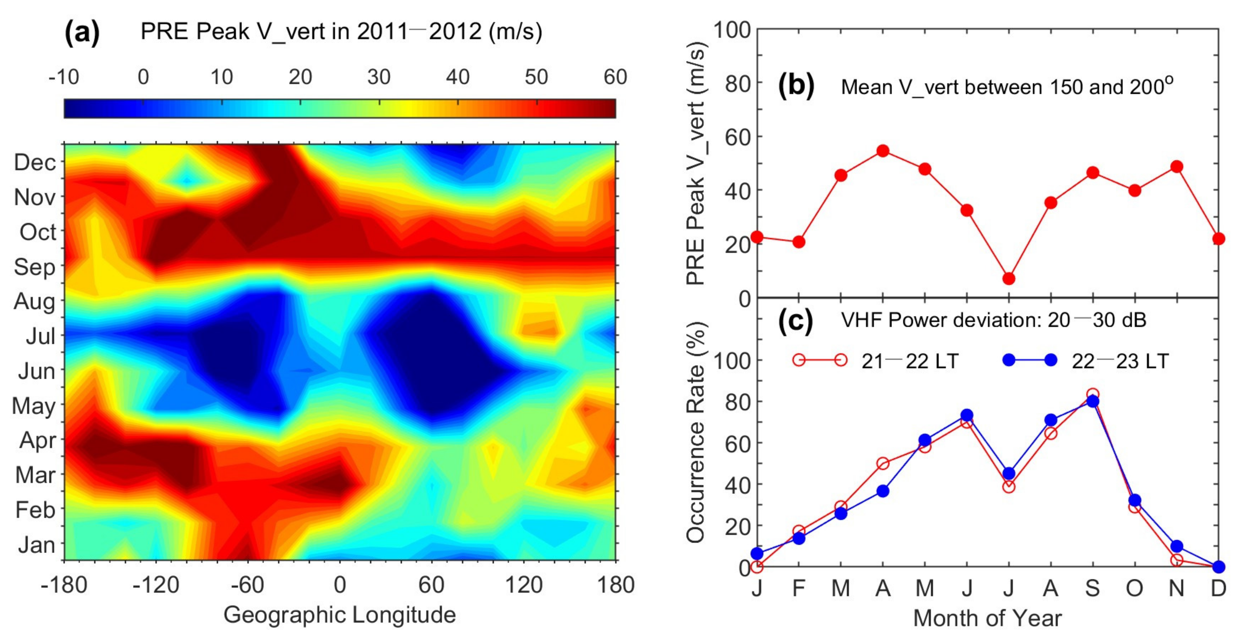
Figure 7a shows the monthly longitudinal distribution of the PRE peak (or the maximum ion drift between 1800 and 1900 LT). The prominent features in
Figure 7a are the minima around ±60° in May–August and the maxima in Equinoxes. However, the PRE peak drift during June solstice became relatively large in the Pacific sector. We are interested in comparing the PRE drift with the scintillation occurrence over Kwajalein. Thus, we selected the PRE peak drift data in the longitudinal range of 150°–200°, and the average values of the drifts are plotted in
Figure 7b. The monthly averaged drifts are large during March–June and September–December but become small in July. The monthly variation of the PRE drift is similar to the variation of the scintillation occurrence probability over Kwajalein (
Figure 7c). Note that the PRE drifts in
Figure 7b are derived over a longitudinal range of 50° (from 150°–200°) from two years (2011–2012) but not exactly over Kwajalein, which may result in the subtle differences between
Figure 7b,c. The general agreement between the PRE drift and the scintillation occurrence provides further evidence that the enhanced PRE drift causes the generation of ionospheric irregularities through plasma bubbles, leading to the occurrence of enhanced scintillation activity. The agreement in the monthly variation of the PRE drift and the scintillation occurrence over Kwajalein is identified for the first time.
4. Discussion
The monthly variation of the occurrence probability of scintillation over Kwajalein, as represented by the S4 index in
Figure 3, shows interesting features (e.g., the variation of the scintillation occurrence with month, local time, and amplitude) that are different from, or not identified in, previous studies. Ref. [
14] analyzed VHF/UHF amplitude scintillation data received at Kwajalein between May, 1976 and November, 1977, and found that the occurrence probability had two maxima in May and July/August and a minimum in June. In contrast,
Figure 3 shows that the occurrence probability of VHF amplitude scintillation was at a maximum in June, 2012 and a minimum in July, 2012. The solar radio flux was low (~80) during the solar minimum year of 1976 and began to increase in 1977. During 2012, the solar flux varied between 100 and 180. It is not certain whether the difference between our study and the result of Ref. [
14] is a consequence of solar activity or whether the monthly occurrence of VHF scintillation at Kwajalein (as well as in other places) varies with year. Addressing this question would require a statistical analysis of scintillation over many years, which is beyond the current research.
Another important feature revealed in
Figure 3a is that the occurrence probability of S4 in the post-midnight sector, represented by the green symbols, was large only in June but not in September. In other words, strong scintillation occurred in the evening sector both in June and September but existed in the post-midnight sector only in June. Two processes might have potentially contributed to this phenomenon. One process is that the decay of scintillation patches was slower in June than in other months. If the background atmospheric density is low, plasma structures might last longer due to a lower recombination rate between ions and neutrals. Another process is that more ionospheric irregularities (and the resultant scintillation) might have been generated in the post-midnight sector in June.
The monthly distribution of VHF scintillation also shows strong dependence on the level of scintillation, as presented in the left column of
Figure 3. A prominent feature is that the occurrence probability is very small at S4 = 0.4–0.8 (
Figure 3b). This phenomenon may be related to the generation of plasma bubbles during high solar activity. As can be seen in
Figure 6, the ESF occurrence probability was high for Δ
N > 3 × 10
10 m
−3 (
Figure 6a), small for Δ
N = 2–3 × 10
10 m
−3 (
Figure 6b), and irregular for Δ
N = 1–2 × 10
10 m
−3 (
Figure 6c). The dependence of the ESF occurrence probability on the irregularity amplitude is the same as the dependence of the scintillation occurrence probability on the scintillation (S4) level, providing clear evidence that the strength of the scintillation is directly related to the amplitude of ionospheric irregularities.
In the study presented in Ref. [
21], the longitude–month distribution of the occurrence probability of ESF irregularities at different levels was derived. Six levels of Δ
N were selected, with Δ
N > 1 × 10
10, 2 × 10
10, 3 × 10
10, 4 × 10
10, 5 × 10
10, and 1 × 10
11 m
−3, respectively. It was found that the patterns of the ESF occurrence probability at high Δ
N levels (Δ
N > 2 × 10
10 and higher) are very similar, and they are different from those at low Δ
N levels (Δ
N > 1 × 10
10). Ref. [
21] suggested that the Rayleigh–Taylor instability can grow into fully developed plasma bubbles and large-amplitude density perturbations in the regions of the large vertical plasma drift. When ESF irregularities with Δ
N > 2 × 10
10 m
−3 are generated in these regions, they often grow into larger amplitudes. In other regions with small vertical plasma drift or downward drift, the growth rate of the Rayleigh–Taylor instability is small, and plasma density perturbations are often small.
This mechanism for the generation of large-amplitude ESF irregularities can be used to explain the occurrence of VHF scintillation. As shown in the left column of
Figure 3, the occurrence probability of S4 > 0.8 is high, but the occurrence probability of S4 at the level of 0.4–0.8 is small. Strong scintillation is caused by large-amplitude irregularities. When ionospheric irregularities grow and cause scintillation at S4 = 0.4–0.8, the irregularities may further grow into larger amplitude and cause stronger scintillation with S4 > 0.8, resulting in a large occurrence rate of scintillation at S4 > 0.8 and a small occurrence rate of scintillation at S4 = 0.4–0.8. The irregular distribution of the occurrence probability of scintillation at S4 = 0.1–0.4 in
Figure 3c may be related to small-amplitude ionospheric irregularities that also have irregular occurrence probability in month and longitude (
Figure 6c). The dependence of the scintillation occurrence rate on the amplitude of S4 is seen for the first time and the direct comparison in the monthly variation between VHF scintillation and ionospheric irregularities is made for the first time.
It is necessary to mention that the monthly distribution of scintillation occurrence is very different for S4 (or scintillation intensity,
SI) greater than a specific value or in a specific range. As can be seen in
Figure 3, the monthly occurrence is similar for S4 > 0.1, 0.4, 0.8, and 1.0. This is because the monthly distribution of scintillation occurrence is dominated by those with large S4 (e.g., S4 > 0.8). If we only look at
Figure 3e (S4 > 0.4), it does not show how scintillation activities at different S4 levels contribute to this distribution. In contrast, if we examine
Figure 3a,b, it becomes clear that the scintillation activity with S4 > 0.8 determines the peaks in June and September.
In this study, we used two criteria (∆
N and
σ) to derive the ESF occurrence probability and found that large-amplitude ESF irregularities over Kwajalein had high occurrence probability in May/June and September in 2012, corresponding to the peaks of VHF scintillation occurrence. However, previous studies found that the ESF occurrence probability over Kwajalein had two maxima in April/May and September and one minimum in June, as compiled by Ref. [
23]. These previous studies used
σ to define ESF. As can be seen in
Figure 6d, the ESF occurrence probability defined by
σ indeed had a minimum in June in the pre-midnight sector (21:00–23:00 LT), which is somewhat similar to the previous results. The June minimum in the ESF occurrence in the previous studies may be related to the definition of ESF.
Both ∆
N and
σ can be used to define ESF irregularities. A unique feature in ESF irregularities defined by
σ is that the ESF occurrence probability is high during local times and seasons when the background plasma density is low. This is understandable because
σ is essentially equal to ∆
N/N and becomes large when
N is small. Ref. [
11] analyzed C/NOFS data and found that the occurrence probability of ESF defined by
σ is low in the evening sector but becomes very high in the post-midnight sector in the months of June solstice during the deep solar minimum period (2008–2010). This feature can also be seen in
Figure 5.
However, for scintillation studies, the definition of ESF irregularities becomes an important issue. It is well understood that scintillation is caused by ionospheric irregularities, and scintillation occurrence is often compared with ESF occurrence. ESF and the resultant scintillation are strong and have high occurrence rates in the evening sector. In this sector, the occurrence probability is high for ESF irregularities defined by ∆
N but low for ESF irregularities defined by
σ. This is because the background plasma density is high there. Ref. [
11] compared the global distribution of ESF occurrence based on ∆
N with S4 and found good agreement.


