Article

Modeling of Organic Aerosol in Seoul Using CMAQ with AERO7

1
Department of Environmental Engineering, Inha University, Incheon 22212, Republic of Korea
2
Air Quality Forecasting Center, National Institute of Environmental Research (NIER), Incheon 22689, Republic of Korea
*
Author to whom correspondence should be addressed.
Atmosphere 2023, 14(5), 874; https://doi.org/10.3390/atmos14050874
Submission received: 29 March 2023 / Revised: 12 May 2023 / Accepted: 15 May 2023 / Published: 16 May 2023
(This article belongs to the Special Issue Air Quality Prediction and Modeling)

Abstract

:
The Community Multiscale Air Quality (CMAQ) model with the 7th generation aerosol module (AERO7) was employed to simulate organic aerosol (OA) in Seoul, Korea, for the year 2016. The goal of the present study includes the 1-year simulation of OA using WRF-CMAQ with recently EPA-developed AERO7 with pcVOC (potential VOC from combustion) scale factor revision and analysis of the seasonal behavior of OA surrogate species in Seoul. The AERO7, the most recent version of the aerosol module of the CMAQ model, includes a new secondary organic aerosol (SOA) species, pcSOA (potential SOA from combustion), to resolve the inherent under-prediction problem of OA. The AERO7 classified OA into three groups: primary organic aerosol (POA), anthropogenic SOA (ASOA), and biogenic SOA (BSOA). Each OA group was further classified into 6~15 individual OA surrogate species according to volatility and oxygen content to model the aging of OA and the formation of SOA. The hourly emissions of POA and SOA precursors were compiled and fed into the CMAQ to successfully simulate seasonal variations of OA compositions and ambient organic-matter to organic-carbon ratios (OM/OC). The model simulation showed that the POA and ASOA were major organic groups in the cool months (from November to March) while BSOA was a major organic group in the warm months (from April to October) in Seoul. The simulated OM/OCs ranged from 1.5~2.1 in Seoul, which agreed well with AMS measurements in Seoul in May 2016.

1. Introduction

PM2.5 (particulate matter with an aerodynamic diameter of less than 2.5μm) harms human health [1,2] and degrades visibility [3,4]. Organic aerosol (OA) is a major chemical component of PM2.5 in most urban areas. OA accounts for 21~69% of the submicron particulate matter mass at the 30 monitoring sites in the Northern Hemisphere [5] and accounts for 10~40% of PM2.5 mass in Korea [6,7,8,9,10].
Primary organic aerosol (POA) is emitted directly from emission sources and secondary organic aerosol (SOA) is formed from volatile organic compound (VOC) precursors. Various aerosol modules simulating the aging of OA and the formation of SOA have been developed and incorporated into chemical transport models [11,12,13,14,15,16,17]. AERO is an aerosol module for the Community Multiscale Air Quality Model (CMAQ; [18]); AERO2 (2nd generation of AERO) is the first version of AERO including POA and SOA with simple SOA forming reactions [19]. AERO3 improves the SOA treatment by including semivolatile compounds partitioning between gas and aerosol phases [20].
As the CMAQ with AERO3 and AERO4 tended to underpredict the OA concentration [21,22], many laboratory and modeling studies were made to discover new pathways for SOA formation. AERO5 adds isoprene, sesquiterpenes, benzene, glyoxal, and methylglyoxal as new SOA precursors based on the work of Edney et al. [23] and Carlton et al. [24]. Despite the expansion of SOA precursors, the underprediction of CMAQ was not fully resolved and further expansion or update of SOA yield was recommended [14,25].
The AERO7, a newly formulated aerosol module [26], introduced a new SOA precursor named pcVOC, potential VOC from combustion, which forms potential SOA from combustion (pcSOA; [27]) through OH oxidation reactions. Similarly, Zhao et al. [28] and An et al. [29] proposed semivolatile/intermediate-volatility organic compounds (S/IVOC) from combustion sources as SOA precursors instead of pcVOC. On the other hand, organic emissions from volatile organic products (VCPs) may contribute to SOA formation [30,31,32]. All of these three schemes are able to produce SOA large enough to eliminate the underprediction. The emissions and oxidation mechanisms of pcSOA, S/IVOC, and VCPs are susceptible to uncertainty. Therefore, mathematical modeling of SOA using air quality models requires a careful estimation of parameters related to SOA formation using observation data.
Although the AERO7 adapted new SOA parameters, there are few studies conducting annual OA simulation using AERO7 in Korea and comparing modeled OA by AERO7 to observations. The present work was aimed at the simulation of OA using WRF-CMAQ with recently EPA-developed AERO7 with revision of the parameter of pcVOC, performance evaluation in predicting OA surrogate species, and the analysis of seasonal behaviors of OA surrogate species in Seoul. The model performance was evaluated using PM supersite monitoring data to optimize the pcSOA-related parameters. The PM supersites in KOREA monitor carbonaceous aerosol mass using the thermal/optical carbon analyzer based on the NIOSH 5040 method for routine monitoring. The mass of total organic carbon (OC) is measured without differentiating primary and secondary components. The elemental carbon (EC) tracer method [33] was applied to estimate the primary and secondary organic carbon (POC and SOC) from the total OC and EC observation data and to compare them to the model results.

2. Materials and Methods

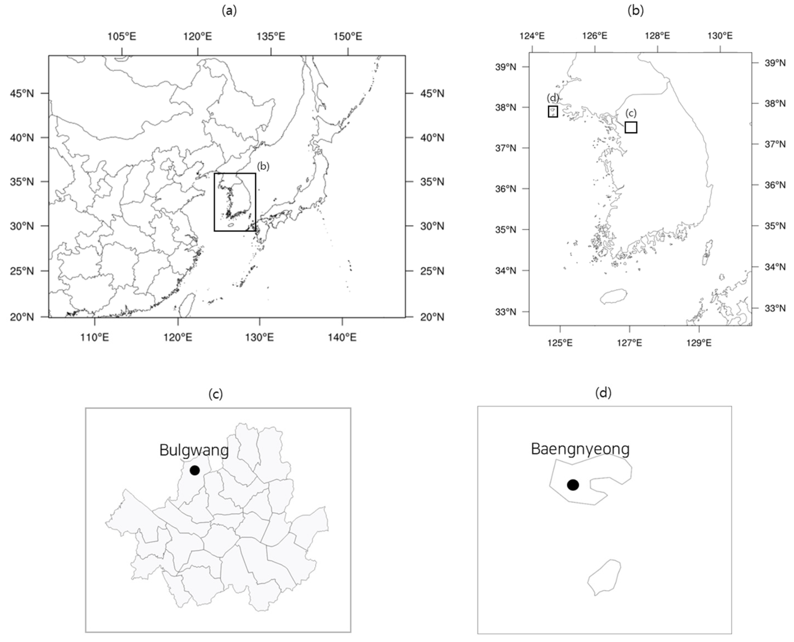
2.1. Monitoring of Carbonaceous Aerosol and Estimation of the Secondary Organic Aerosol Concentration

The Korean Ministry of Environment established ten PM2.5 supersites to routinely monitor hourly PM2.5 chemical compositions, sulfate, nitrate, ammonium, OC, EC, and minerals. The data used for model verification were collected from two Korean PM supersites, the Bulgwang (BG) and Baengnyeong (BN) sites. The BG site is an urban site located in the North of Seoul and the BN site is a remote site located in the upwind region of Seoul as shown in Figure 1.
OA is directly emitted into the air (POA) or formed in the atmosphere through the photochemical oxidation of organic gases and subsequent gas/particle partitioning (SOA). POA and SOA have different origins and different impacts on human health [34]. Therefore, designing cost-effective mitigation strategies requires information on POA and SOA ratios.
A state-of-the-art instrument including an aerosol mass spectrometer (AMS) has been recently developed to investigate POA and SOA separately, but the cost of its installation and operation limits the number of monitoring sites and the monitoring duration. Instead, a thermal/optical carbon analyzer has been used for routine monitoring [35] by most institutes including the PM2.5 chemical speciation network (CSN) of the US-EPA, the European Supersites for Atmospheric Aerosol Research (EUSAAR), and Korean PM2.5 supersites [36].
The thermal/optical carbon analyzer uses the NIOSH 5040 method for separating organic carbons from inorganic carbons and the non-dispersive infrared method for the analysis of CO2 generated from the combustion of organic and inorganic carbon. It measures the mass of OC instead of the organic matter (OM) without differentiating primary and secondary components. Turpin and Huntzicker [33] proposed the EC tracer method, which assumes a linear relationship between the POC and EC concentrations. Then, the POC concentration can be estimated by:
[POC] = a + b [EC]
The intercept “a” represents the non-combustion POC concentration and the slope “b” becomes the POC to EC mass concentration ratio (POC/EC) if “a” is negligible. The POC concentration may be approximated by the OC concentration in the SOC-free conditions to yield:
[OC]SOC-free = a + b [EC]
Meteorological conditions or OC to EC concentration ratios (OC/EC) were used to choose the SOC-free case [33,35,37]. In the present work, the data with OC/EC less than their fifth percentile values were chosen as a subset of the SOC-free case. The regression analysis method was applied to this subset to determine “a” and “b”. Because both the SOC-free OC concentration and the EC concentration may have non-negligible uncertainties, the Deming regression method was used instead of the ordinary linear regression method. In addition, the uncertainties of OC and EC concentrations were assumed to be equal following the previous work [37].
Once “a” and “b” are determined, one can calculate the POC concentration from the observed EC concentration using Equation (1) and subsequently the SOC concentration using:
[SOC] = [OC] − [POC]
We compared the SOC concentrations estimated by Equation (3) with those predicted by the air quality model for model validation.

2.2. Model Simulation and Performance Evaluation

WRF (Weather Research and Forecast) version 3.6 and CMAQ (Community Multiscale Air Quality) version 5.3.1 were used to model the PM2.5 mass and chemical compositions. The Global to Mesoscale Air Quality Forecast and Analysis (GMAF) framework [38] was employed to assign initial and boundary conditions and to carry out a grid nudging-based four-dimensional data assimilation (FDDA) for CMAQ and WRF modeling. The 0.25° Global Data Assimilation System (GDAS) dataset was used for the WRF and the 0.4° Copernicus Atmospheric Monitoring Service (CAMS) dataset for the CMAQ [39].
The 7th generation aerosol module (AERO7) was used as an aerosol module and the 3rd release of the carbon bond mechanism version 6 (CB6r3; [40]) was used as the gas-phase chemical mechanism. The WRF is configured as follows: YSU PBL scheme for the planetary boundary layer, Revised MM5 surface layer scheme for the surface layer, Unified Noah land surface model for the land surface model, WSM6 microphysics scheme for the microphysics, Kain–Fritsch cumulus convection for the cumulus parameterization, the Goddard shortwave radiation scheme for the shortwave radiation, and the RRTM longwave radiation scheme for the longwave radiation.
A nested grid domain system was adopted: 27 km grid spacing for the outer domain and 9 km grid spacing for the inner domain. The outer domain covers the Korean peninsula, eastern and southern China, part of Russia, and Japan. The study area shown in Figure 1 was taken as the inner domain, which includes South Korea and a part of North Korea. The modeling period is from 1 December 2015 to 30 November 2016, covering one whole year.
The model performance was evaluated by three statistical metrics: the correlation coefficient (R), the normalized mean error (NME), and the normalized mean bias (NMB). The formulas of the statistical metrics are:
R = i = 1 i = N ( O i O ¯ ) ( M i M ¯ ) i = 1 i = N ( O i O ¯ ) 2 i = 1 i = N ( M i M ¯ ) 2
NME   ( % ) = 1 N i = 1 i = N | M i O i | O ¯ × 100
NMB   ( % ) = M ¯ O ¯ O ¯ × 100
where subscript ‘O’ and ‘M’ denote the observation and the model prediction, respectively. ‘N’ is the total number of paired datasets. The overbar indicates an average value. Emery et al. [41] reviewed modeling studies carried out in the United States of America (USA) and recommended a set of numerical “goals” and less restrictive “criteria” for the R, the NME, and the NMB for the evaluation of chemical transport models. We used these goals and criteria for model verification as described in Section 3.1.

2.3. Atmospheric Aerosol Chemistry
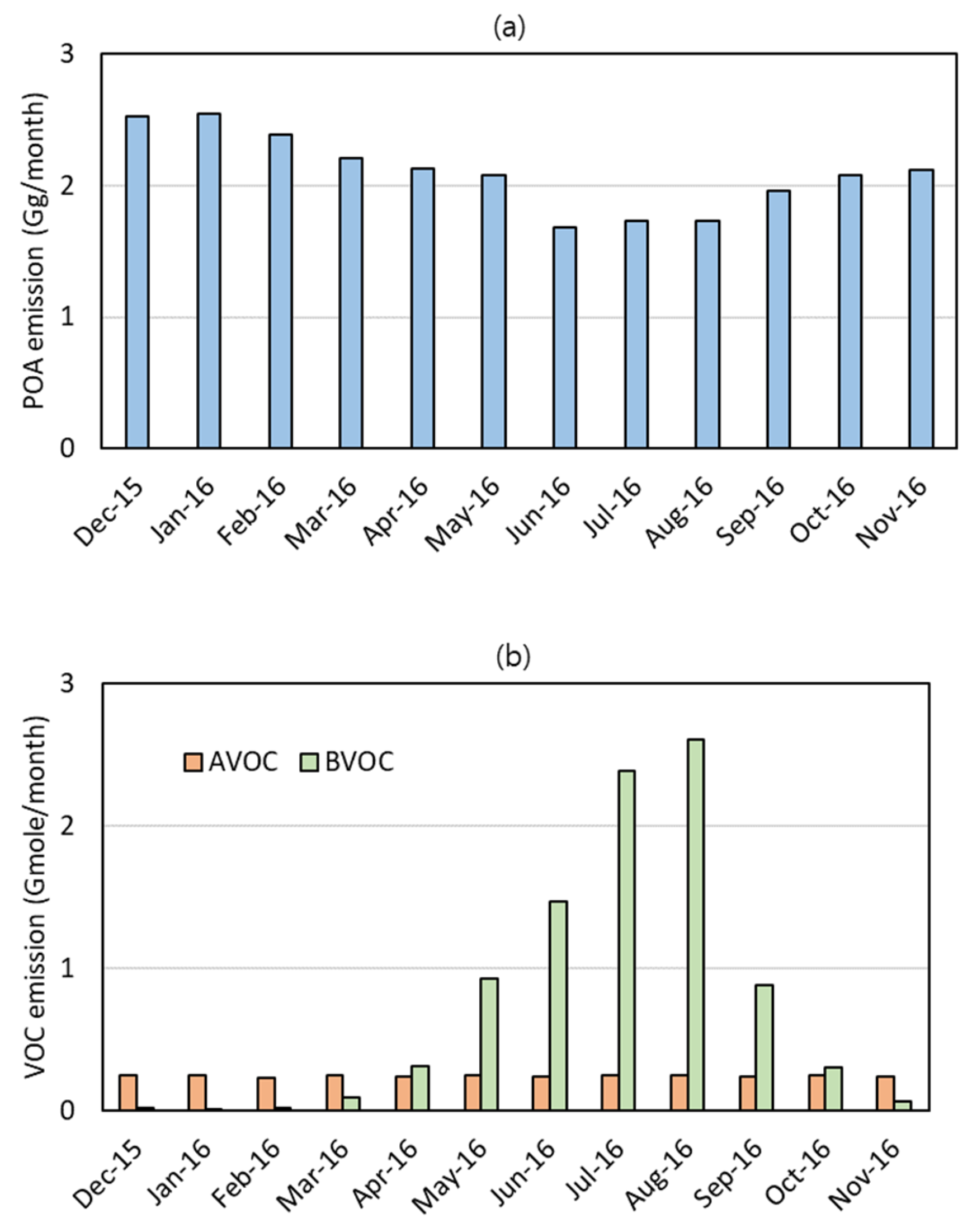
The AERO7 categorized the OA into POA, anthropogenic SOA (ASOA), and biogenic SOA (BSOA). Each OA category was further classified according to the scheme of the volatility basis set (VBS; [42,43]). The POA is composed of the directly emitted POA (EPOA) and their oxidation products (OPOA). Each of the EPOA and OPOA has five surrogate species with varying of volatility, effective saturation concentration (C*), oxygen to carbon ratio (O/C), and OM to OC ratio (OM/OC) as listed in Table 1 [27]. The C* of EPOA surrogate species, an indicator of volatility, was set to range from 0.1 to 1000 μg/m3. The EPOA surrogate species have a high carbon content such that O/Cs and OM/OCs are low. The OPOA surrogate species are formed from the oxidation products of EPOA, which results in lower volatility and higher O/Cs and OM/OCs than the EPOA surrogate species.
Anthropogenic SOA (ASOA) is formed from the oxidation products of anthropogenic VOC (AVOC) gases, which includes toluene, xylene, benzene, PAH (polycyclic aromatic hydrocarbon), and potential VOC from combustion (pcVOC). A previous version of the aerosol module tended to underestimate the SOA mass. The AERO7 postulated that the SOA-forming VOCs emitted from combustion were not fully accounted for and introduced the pcVOC as a new VOC surrogate species [27]. pcVOC reacts with the OH radical to form a low-volatility potential secondary organic gas from combustion emissions (pcSOG), which condenses to become the potential SOA from combustion (pcSOA). The AERO7 presumed that the pcVOC emission is proportional to the POA emissions and calculated the pcVOC emission by multiplying the POA emission by a pcVOC emission scale factor. There is no theoretical way to determine a pcVOC emission scale factor. In this work, the pcVOC emission scale factor was set to 0.0155 mole-pcVOC/g-POA based on the sensitivity runs made for Korea by Cho et al. [38].
The 6th generation aerosol module (AERO6) explicitly models the transformation of AVOCs with over twenty ASOA species. The AERO7 lumped these explicit ASOA species into four ASOA surrogate species, named AAVB1~AAVB4, according to the VBS scheme as shown in Table 2. AAVB1 has the lowest volatility with the C* of 0.01 μg/m3, and the C* values of AAVB2, AAVB3, AAVB4 are 100, 1000, and 10,000 times the C* of AAVB1, respectively. AAVB1~AAVB4 have O/Cs in the range of 0.659~1.227 and OM/OCs in the range of 1.99~2.70, which are similar to those of the OPOA. AAVB2, AAVB3, and AAVB4 form oligomer products of ASOA compounds (AOLGA). The values of C*, O/C, and OM/OC of AOLGA are 10−10 μg/m3, 1.067, and 2.5, respectively. pcSOA has low volatility with the C* of 10−5 μg/m3, and the values of O/C and OM/OC of the pcSOA are 0.667 and 2, respectively.
The VOCs released from plants are called biogenic VOCs (BVOCs), which include monoterpenes, sesquiterpenes, isoprene, glyoxal, and methylglyoxal. BVOCs produce gas-phase oxidation products via photochemical degradation. Various heterogeneous reactions of these gaseous precursors form the biogenic SOA (BSOA) [44]. The AERO7 models these processes by 15 BSOA surrogate species as listed in Table 3. The monoterpene surrogate species in the AERO7 were divided into six volatility bins according to the VBS scheme (AMT1~AMT6). In addition, the organic nitrate from monoterpene oxidation (AMTNO3) and its hydrolysis product (AMTHYD) were added to the BSOA to account for high SOA yields from organic nitrates observed in the southeastern USA [45]. The O/Cs and the OM/OCs of AMT1~AMT6, AMTNO3, and AMTHYD are lower than those of the ASOA surrogate species. The O/C and the OM/OC of the ASQT are similar to those of the monoterpene surrogate species. On the other hand, the O/Cs and the OM/OCs of the isoprene surrogate species (AISO1, AISO2, and AISO3) are higher than those of the monoterpene surrogate species and similar to those of the ASOA surrogate species. ASQT, AISO1, and AISO2 form oligomer products of BSOA compounds, AOLGB. AOLGB has low volatility with C* equal to 10−10 μg/m3 and with the OM/OC equal to 2.1. AGLY and AORGC are produced from aerosol uptakes and in-cloud processing of glyoxal and methylglyoxal, respectively. They also have low volatility with C* equal to 10−10 μg/m3 and with OM/OCs equal to 2.13 and 2.00, respectively.

2.4. Emissions

The Korean–United States Air Quality Study (KORUS-AQ) version 2.1 emission inventory was used for the anthropogenic emissions of the Northeastern Asian region and the Clean Air Policy Support System (CAPSS) emission inventory was used for the anthropogenic emissions of Korea. The base year of both emission inventories was 2016. The natural emissions were estimated by the Model of Emissions of Gases and Aerosols from Nature (MEGAN) version 2.l [46].
Figure 2 shows the monthly emissions of POA, AVOCs, and BVOCs in the Korea model domain. The POA was mainly emitted from mobile sources, industrial combustion, and residential and commercial heating. As shown in Figure 1a, the Korea model domain includes a part of North Korea, where residential heating emitted a large amount of POA in the cool months (from November to March).
The emissions of AVOCs, defined as anthropogenic VOCs forming ASOA in this work, consisted of 66% toluene, 21% xylene, and 13% pcVOC with negligibly small benzene, PAHs, and long-chain alkanes. The monthly average emissions of pcVOC occupy the AVOCs emissions by 11% in August and 16% in January: small in the warm months (from April to September) and large in the cool months. On the contrary, the monthly average emissions of toluene and xylene in the warm months were larger than those in the cool months, offsetting the seasonal variation of pcVOC. As a result, the monthly average AVOC emissions changed by only less than 6% over the year.
Isoprene and terpenes together comprise most of the BVOC emissions in the Korea model domain. The isoprene and terpene emissions increase exponentially with temperature [47,48] and peak in the warm months. This seasonal change made the BVOCs dominate in the warm months while the AVOCs dominated in the cool months, as also shown in Figure 2b.

3. Results and Discussion

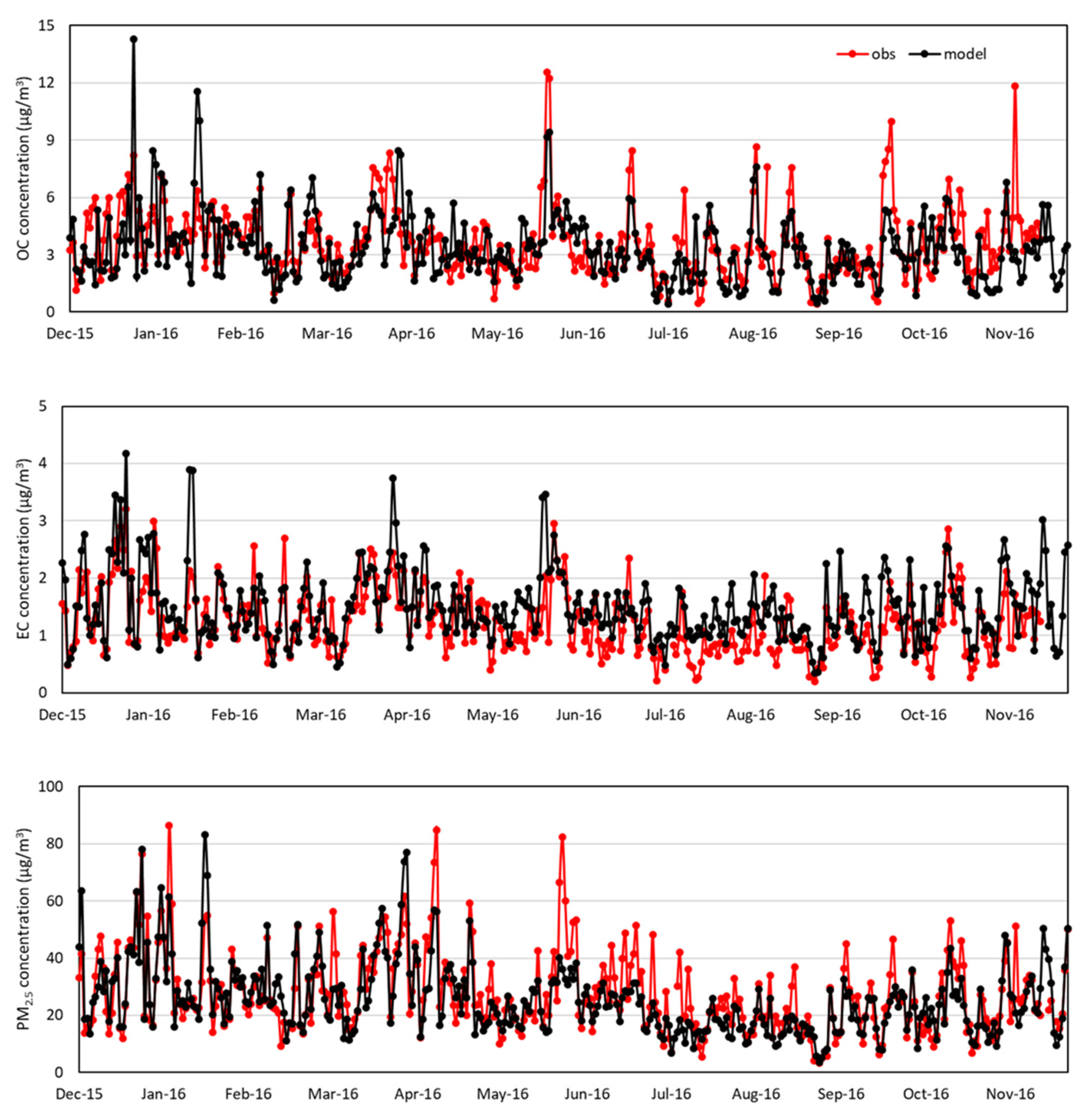
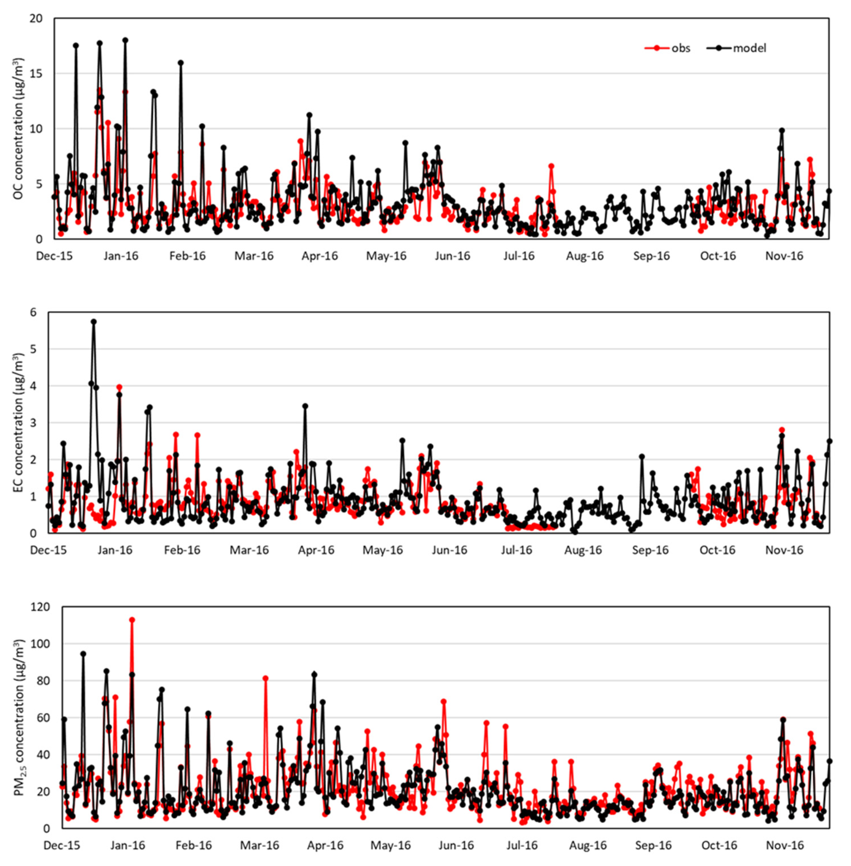
3.1. Model Evaluation on OC and EC Prediction

Detailed model performance evaluation on various meteorological parameters and inorganic chemical components including sulfate, nitrate, and ammonium have been presented elsewhere [38,49]. Therefore, we limited model validation to carbonaceous aerosol component mass and PM2.5 mass.
Table 4 compares the annual average concentrations of observed and modeled OC, EC, and PM2.5 concentrations in two supersites, the BG and BN sites. In addition, the model performance metrics are also presented. The observed OC, EC, and PM2.5 concentrations at the BG site, an urban site, are higher than those at the BN site, a remote site. As the individual component concentrations add up, the associated errors often cancel each other to improve the overall performance statistics. The correlation coefficient (R), normalized mean error (NME), and normalized mean bias (NMB) of PM2.5 appeared better than those of OC and EC. The R of PM2.5 was 0.81 for the BG site and 0.75 for the BN site, exceeding the goal (>0.7) set by Emery et al. [41]. The Rs of OC and EC were slightly lower than the R of PM2.5 in most of the cases, and they were deemed reasonably good.
The NMEs of OC and EC satisfy the accuracy goal (<45% for OC and <50% for EC). In addition, the NMBs of OC and EC mostly meet the accuracy goal (<±15% for OC and <±20% for EC). Despite differences in the site characteristics between the BG and BN sites, there are no systematic differences in R, NME, and NMB between these two sites. Therefore, it may be concluded that the modeled OC and EC concentrations agree reasonably well with the observation.
Figure 3 and Figure 4 compare daily variations of OC, EC, and PM2.5 concentrations between observations and modeling at the BG and BN sites. At the BG site, the modeled OC, EC, and PM2.5 closely follow the observed ones except for the warm months during which the model underestimates the OC and PM2.5 and overestimates the EC. At the BN site shown in Figure 4, the modeled OC, EC, and PM2.5 closely follow the observed ones except for the cool months during which the model overestimates the peaks.

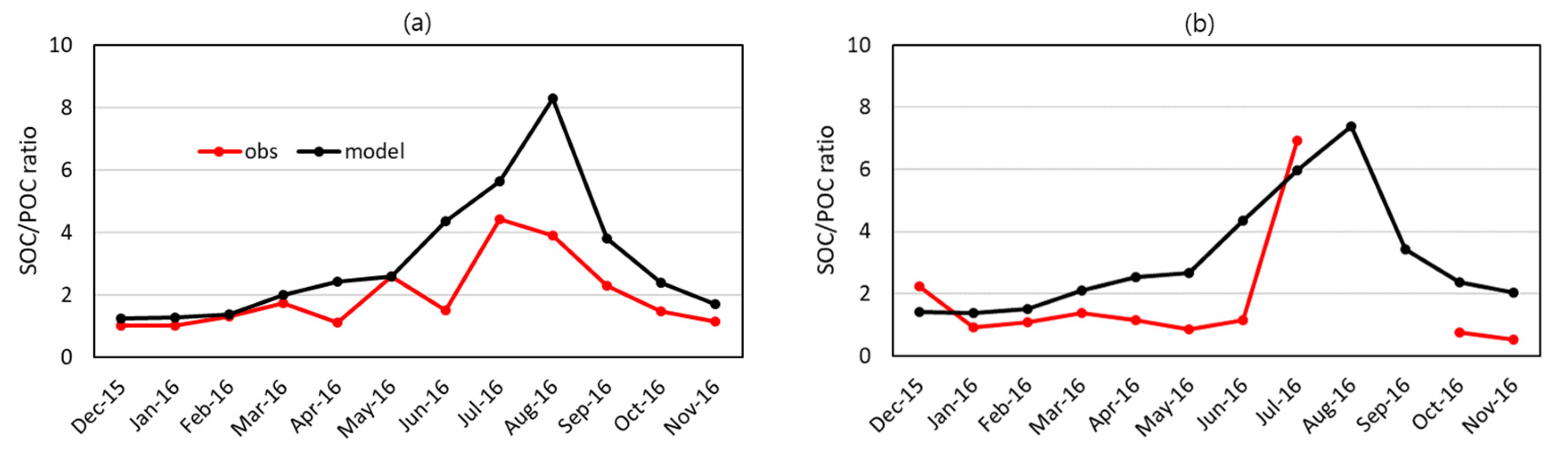
3.2. Model Evaluation on SOC Prediction

The EC tracer method described in Section 2.1 assumes the POC to EC concentration ratio (POC/EC) to be spatially and temporally constant. However, the POC/EC changes with the source types; the POC/ECs of aerosol from biomass burning cover a range of 2.6~5.7; those from fossil fuel combustion are lower than 1 [35]. Therefore, an analysis period should be appropriately set; it should be short enough to have only one type of source dominate, and at the same time, it should be long enough to have a sufficient number of data available for the regression analysis. In this study, we took one month as an analysis period and applied a regression analysis to monitored the concentrations of OC and EC hourly.
Table 5 lists the Deming linear regression analysis results, the standard errors of the regression, and the Rs at two PM supersites, the BG and BN sites, the site location and the site characteristics of which were presented in Section 2.1. The plots of the Deming linear regression analysis results for the BG and BN sites can be found in Figure S1 and Figure S2. The magnitude of intercept at both sites is one order magnitude smaller than the POC concentration, the dependent variable, and the Rs between the POC and EC concentrations are greater than 0.9 in most months. The averaged standard errors of the regression at the BG site are smaller than 0.73 μg/m3, and those at the BN site are smaller than 0.44 μg/m3. In addition, we used the slope as an estimate of POC/EC like the previous works [35,37,50].
The slopes, POC/ECs, range from 0.78 to 2.02 at the BG site, an urban site. The slopes are higher in the cool months (from November to March) than in the warm months (from April to October) because of the stronger effects of biomass burning in the cool months as pointed out by Pio et al. [35]. The slopes at the BN site, a remote site, are bigger than those at the BG site due to the greater contribution from biomass burning.
The EC tracer method parameters, slope and intercept, listed in Table 5 were used to calculate the monthly values of SOC to POC concentration ratios (SOC/POCs) from the OC concentrations monitored at the BG and BN sites. Figure 5 compares the SOC/POCs directly calculated by CMAQ to the EC tracer method. At the BG monitoring site, the estimated monthly SOC/POCs were 1.0~1.3 in the cool months and increased in the warm months, reaching the maximum of 4.4 in July. The modeled ratios were in good agreement with the estimated ones in the cool months. In the warm months, BVOCs emitted from plants increased to form more SOC to increase the values of SOC/POCs. The modeled and observed values of SOC/POCs at the BN site behave similarly to those at the BG site especially in the cool months, thus exhibiting the regional characteristics of SOC/POC.
The POC and SOC concentrations from modeling are compared to those estimated by the EC tracer method as shown in Table 6. The performance metrics including R, NME, and NMB are also presented. The model performance of individual components tends to degrade as the OC is divided into POC and SOC, resulting in the R, NME, and NMB of the POC and SOC being lower than those of the OC, as shown in Table 4. The NMEs and NMBs of POC and SOC mostly satisfy their accuracy criteria for OC (<65% for NME, <±50% for NMB). Because the threshold values of NME and NMB of the individual OC species are expected to be lower than those of the total OC, the model performance in predicting the SOC and POC is deemed reasonably good.

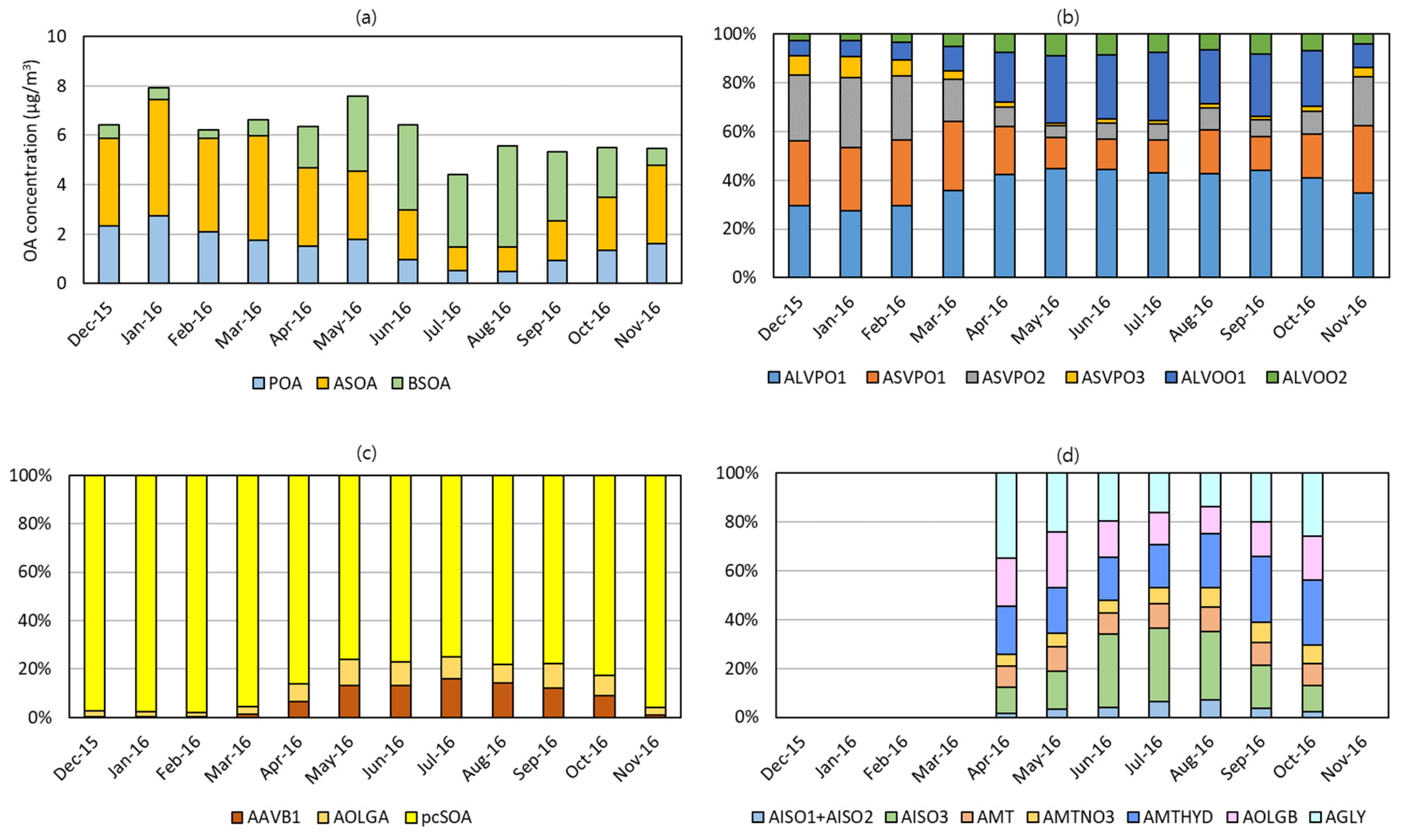
3.3. Modeling of the Seasonal Behavior of Organic Aerosol Compositions

Figure 6a displays the monthly average concentrations of the POA, the ASOA, and the BSOA in Seoul. The POA and the ASOA occupied a larger fraction in the cool months (from November to March), while the BSOA occupied a larger fraction in the warm months (from April to October) due to the seasonal variation in precursor emissions. The monthly average POA concentrations appeared similar to the monthly average ASOA concentrations. In the warm months, the wind direction shifts from the northwest to the southeast to bring the air mass with lower PM2.5, POA, and SOA concentrations. Moreover, the POA emission decreased in the warm months as shown in Figure 2a to promote a further decrease in the POA concentration.
Figure 6b shows the composition profiles of POA; ALVPO1, ASVPO1, ASVPO2, and ASVPO3 are the directly emitted POA (EPOA), and ALVOO1 and ALVOO2 are their oxidation products (OPOA) formed by reacting with the OH radical. In the cool months, the POA was mainly composed of EPOA species due to the weak solar radiation and low OH radical concentration. On the contrary, the relative contribution of OPOA species to the POA concentration increased in the warm months as the solar radiation and the OH radical concentration increased.
As shown in Figure 6c, the pcSOA was a major ASOA species in all seasons as designed, and it reduced the underestimation of ASOA. As noted in Section 2.4, the aromatic gas emissions increased in the warm months while the pcVOC emissions decreased. The AAVB1 and AOLGA are oxidation products of aromatic gases [30] and therefore increased in the warm months to occupy 17~23% of the ASOA.
Figure 6d shows the monthly average compositions of the BSOA. The AISO3, an acid-catalyzed isoprene SOA compound, had the largest percent contribution, and the AGLY, a non-volatile SOA from heterogeneous uptakes of glyoxal and methylglyoxal, and the AMTHYD, a non-volatile organic hydrolysis product of AMTNO3, had the second and third largest contributions in the warm months, respectively. The oxidation of isoprene by the OH radical at a low NOx concentration produces IEPOX (isoprene epoxydiol) and the SOA uptakes the IEPOX to form AISO3 [51]. The production rate of IEPOX increases as the ambient temperature increases [52], which resulted in high concentrations of AISO3 in the warm months. This temperature dependency of AISO3 was also observed by Mahilang et al. [53]. The fractions of AGLY ranged from 14~35% in the warm months, which are significant percent contributions to the SOA formation consistent with previous works [13,45,54]. The oxidation of monoterpene by typical photochemical oxidants (OH radical, O3) and NO3 radical produces AMT1~AMT6 and AMTNO3, respectively. In addition, the hydrolysis reaction converts AMTNO3 to AMTHYD. As reported by previous works [45,55], the SOA yields from oxidation by NO3 radical were generally higher than those by the OH radical and O3, and therefore the sum of the AMTNO3 and AMTHYD concentrations was larger than AMT1~AMT6 as also shown in Figure 6d. The oligomer products from BSOA, AOLGB, occupied 13~23% of the BSOA during the warm months.

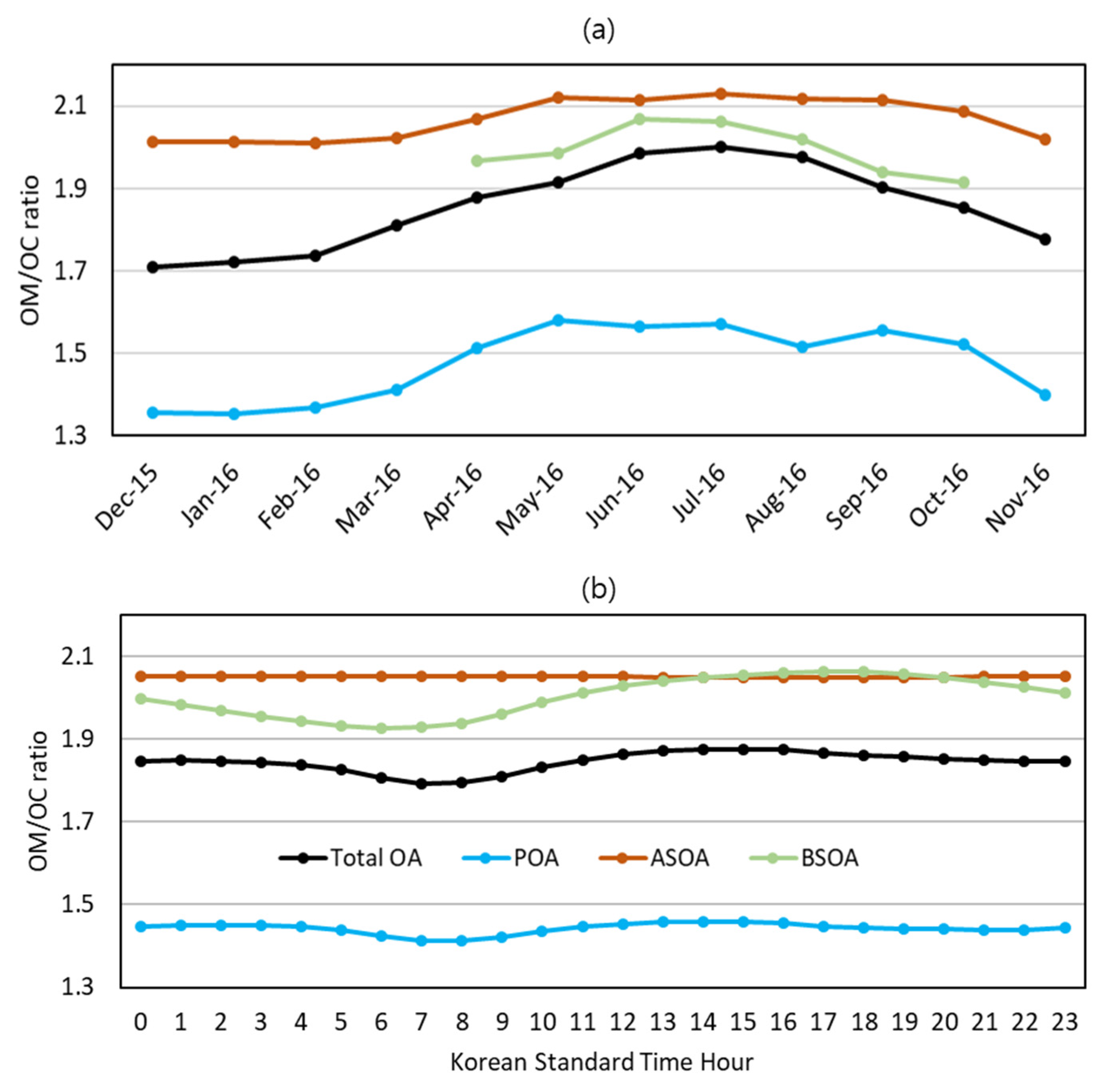
3.4. Organic Matter to Organic Carbon Ratio

The organic matter to organic carbon ratios (OM/OCs) were calculated using aerosol surrogate species concentrations predicted by the CMAQ with AERO7. As shown in Figure 7a, the monthly average OM/OCs of total OA ranged between 1.7~2.1, which is consistent with the AMS monitoring data [56]. In the warm months, strong solar radiation accelerated the photochemical oxidation of OAs to increase the monthly average OM/OCs of total OA to as high as 2.0. The monthly average OM/OCs dropped to as low as 1.7 in the cool months.
Additionally displayed in the same figure are the OM/OCs of the OA subgroups, POA, ASOA, and BSOA. They exhibited monthly variations similar to the OM/OCs of the total OA: high in the warm months and low in the cool months. The ASOA has the highest OM/OC and the POA has the lowest OM/OC. The OM/OCs and O/Cs of individual species constituting each subgroup are presented in Table 1 and Table 2. The seasonal variations of the OM/OCs of each subgroup were determined by seasonal changes in chemical constituents. As an oxidation of OAs proceeds, the oxygen atoms are added to the aerosol to increase the OM/OC ratios. Therefore, the concentrations of the highly oxidized form of OA, AAVB1 and AOLGA for ASOA, ALVOO1 for POA, and AISO3 for BSOA, increased in the warm months as shown in Figure 6b–d. As a result, the OM/OCs in the warm months are higher than those in the cool months by approximately 11% for the total OA, 5% for the ASOA, and 13% for the POA.
Figure 7b shows the annually average diurnal variation of the OM/OC of total OA and individual OA groups. The ASOA had the highest OM/OC and the POA had the lowest OM/OC. The diurnal variation was small compared to the annual variation: the daytime average OM/OCs of total OA, POA, ASOA, and BSOA were 1.85, 1.44, 2.05, and 2.02, respectively, approximately the same as the nighttime average OM/OCs.

4. Summary and Conclusions

It is well known that OA is one of the major components of PM2.5 in Korea along with sulfate and nitrate [38,57]. In this work, a newly released aerosol module, the AERO7, was implemented onto CMAQ to simulate the OA for the year of 2016 in Seoul, Korea. The AERO7 introduced a new OA species to reduce the underprediction of OA suffered by the previous aerosol modules. The CMAQ model with AERO7 performs very well, satisfying the accuracy goal or criteria for EC, OC, and PM2.5 concentrations. Moreover, the calculated OM/OCs ranged from 1.5 to 2.1, which agrees well with the AMS measurements in Seoul in May 2016.
The present model simulation shows that the POA and ASOA were major organic groups in the cool months (from November to March) while BSOA was a major organic group in the warm months (from April to October) in Seoul. The seasonal changes in the emissions of POA and VOC precursors appeared to be responsible for the seasonal variations in POA, ASOA, and BSOA. Each OA group, POA, ASOA, and BSOA, consists of 6~15 individual OA surrogate species classified according to volatility and oxygen content. The ambient temperature and solar radiation intensity affect the distribution of individual OA surrogate species within each organic group. In the present work, ALVPO1 maintains the highest fraction the whole year around. In addition, ASVPO1 and ASVPO2 were major POA surrogate species in the cool months whereas ALVOO1 was a major POA surrogate species in the warm months. AISO3, AGLY, AMTHYD, and AOLGB were major BSOA surrogate species and pcSOA was a major ASOA surrogate species.
pcSOA is one of the major OA components, which is formed by the oxidation of pcVOC. The pcVOC emission is estimated by scaling the POA emissions. There is no theoretical way to estimate the pcVOC emission scale factor. Therefore, most works including the present one adjust the scale factor until the modeled OA concentration matches the observed one. It is recommended to have a better representation of pcVOC and compile the emission factors. Other VOC precursors of ASOA rather than pcVOC are aromatics and long-chain alkanes. Model performance evaluation in predicting long-chain alkanes is substantially lacking compared to aromatics, thus requiring future work on emissions and ambient concentration monitoring.

Supplementary Materials

The following are available online at https://www.mdpi.com/article/10.3390/atmos14050874/s1, Figure S1: Monthly Deming regression analysis results in BG supersite, Figure S2: Monthly Deming regression analysis results in BN supersite.

Author Contributions

H.-Y.P. conducted the model simulation and analyzed the results, S.-Y.C. analyzed the results and wrote this paper, S.-C.H. and J.-B.L. contributed to the forecast interpretation and performance evaluation. All authors have read and agreed to the published version of the manuscript.

Funding

This research was funded by the National Institute of Environmental Research of South Korea, grant number: NIER-2022-01-02-072, and supported by a grant from the National Institute of Environmental Research, funded by the Ministry of Environment (MOE) of South Korea, grant number: NIER-2021-03-03-007.

Institutional Review Board Statement

Not applicable.

Informed Consent Statement

Not applicable.

Data Availability Statement

The monitoring data were obtained from the National Institute of Environmental Research (NIER), and they are available from the authors with the permission of NIER.

Acknowledgments

The authors would like to thank the Korean National Institute of Environmental Research for providing the PM supersite data.

Conflicts of Interest

The authors declare no conflict of interest.

References

  1. Dockery, D.W.; Pope, C.A.; Xu, X.; Spengler, J.D.; Ware, J.H.; Fay, M.E.; Ferris, B.G., Jr.; Speizer, F.E. An association between air pollution and mortality in six US cities. N. Engl. J. Med. 1993, 329, 1753–1759. [Google Scholar] [CrossRef]
  2. Pope, C.A.; Thun, M.J.; Namboodiri, M.M.; Dockery, D.W.; Evans, J.S.; Speizer, F.E.; Heath, C.W. Particulate air pollution as a predictor of mortality in a prospective study of US adults. Am. J. Respir. Crit. Care Med. 1995, 151, 669–674. [Google Scholar] [CrossRef] [PubMed]
  3. Pui, D.Y.; Chen, S.-C.; Zuo, Z. PM2.5 in China: Measurements, sources, visibility and health effects, and mitigation. Particuology 2014, 13, 1–26. [Google Scholar] [CrossRef]
  4. Wang, X.; Zhang, R.; Yu, W. The effects of PM2.5 concentrations and relative humidity on atmospheric visibility in Beijing. J. Geophys. Res. Atmos. 2019, 124, 2235–2259. [Google Scholar] [CrossRef]
  5. Jimenez, J.L.; Canagaratna, M.; Donahue, N.; Prevot, A.; Zhang, Q.; Kroll, J.H.; DeCarlo, P.F.; Allan, J.D.; Coe, H.; Ng, N. Evolution of organic aerosols in the atmosphere. Science 2009, 326, 1525–1529. [Google Scholar] [CrossRef] [PubMed]
  6. National Institute of Environmental Research (NIER). Analysis of Characteristics and Formation Mechanism of Fine Particulate Matter (PM2.5) Concentration by Province (I); NIER: Incheon, Republic of Korea, 2011. Available online: https://scienceon.kisti.re.kr/srch/selectPORSrchReport.do?cn=TRKO201300007595 (accessed on 28 March 2023).
  7. Shon, Z.-H.; Kim, K.-H.; Song, S.-K.; Jung, K.; Kim, N.-J.; Lee, J.-B. Relationship between water-soluble ions in PM2.5 and their precursor gases in Seoul megacity. Atmos. Environ. 2012, 59, 540–550. [Google Scholar] [CrossRef]
  8. Lee, Y.-J.; Park, M.-K.; Jung, S.-A.; Kim, S.-J.; Jo, M.-R.; Song, I.-H.; Lyu, Y.-S.; Lim, Y.-J.; Kim, J.-H.; Jung, H.-J.; et al. Characteristics of Particulate Carbon in the Ambient Air in the Korean Peninsula. J. Korean Soc. Atmos. Environ. 2015, 31, 330–344. [Google Scholar] [CrossRef]
  9. Cho, S.-H.; Kim, P.-R.; Han, Y.-J.; Kim, H.-W.; Yi, S.-M. Characteristics of Ionic and Carbonaceous Compounds in PM2.5 and High Concentration Events in Chuncheon, Korea. J. Korean Soc. Atmos. Environ. 2016, 32, 435–447. [Google Scholar] [CrossRef]
  10. Park, E.H.; Heo, J.; Kim, H.; Yi, S.M. The major chemical constituents of PM2.5 and airborne bacterial community phyla in Beijing, Seoul, and Nagasaki. Chemosphere 2020, 254, 126870. [Google Scholar] [CrossRef]
  11. Simon, H.; Bhave, P.V. Simulating the degree of oxidation in atmospheric organic particles. Environ. Sci. Technol. 2012, 46, 331–339. [Google Scholar] [CrossRef]
  12. Li, J.; Cleveland, M.; Ziemba, L.D.; Griffin, R.J.; Barsanti, K.C.; Pankow, J.F.; Ying, Q. Modeling regional secondary organic aerosol using the Master Chemical Mechanism. Atmos. Environ. 2015, 102, 52–61. [Google Scholar] [CrossRef]
  13. Ying, Q.; Li, J.; Kota, S.H. Significant contributions of isoprene to summertime secondary organic aerosol in eastern United States. Environ. Sci. Technol. 2015, 49, 7834–7842. [Google Scholar] [CrossRef] [PubMed]
  14. Li, J.; Zhang, M.; Tang, G.; Sun, Y.; Wu, F.; Xu, Y. Assessment of dicarbonyl contributions to secondary organic aerosols over China using RAMS-CMAQ. Atmos. Chem. Phys. 2019, 19, 6481–6495. [Google Scholar] [CrossRef]
  15. Lee, H.-J.; Jo, H.-Y.; Song, C.-K.; Jo, Y.-J.; Park, S.-Y.; Kim, C.-H. Sensitivity of Simulated PM2.5 Concentrations over Northeast Asia to Different Secondary Organic Aerosol Modules during the KORUS-AQ Campaign. Atmosphere 2020, 11, 1004. [Google Scholar] [CrossRef]
  16. Yu, Z.; Jang, M.; Kim, S.; Son, K.; Han, S.; Madhu, A.; Park, J. Secondary organic aerosol formation via multiphase reaction of hydrocarbons in urban atmospheres using CAMx integrated with the UNIPAR model. Atmos. Chem. Phys. 2022, 22, 9083–9098. [Google Scholar] [CrossRef]
  17. Oak, Y.J.; Park, R.J.; Jo, D.S.; Hodzic, A.; Jimenez, J.L.; Campuzano-Jost, P.; Nault, B.A.; Kim, H.; Kim, H.; Ha, E.S.; et al. Evaluation of Secondary Organic Aerosol (SOA) Simulations for Seoul, Korea. J. Adv. Model. Earth Syst. 2022, 14, e2021MS002760. [Google Scholar] [CrossRef]
  18. Byun, D.; Schere, K.L. Review of the governing equations, computational algorithms, and other components of the Models-3 Community Multiscale Air Quality (CMAQ) modeling system. Appl. Mech. Rev. 2006, 59, 51–77. [Google Scholar] [CrossRef]
  19. Binkowski, F.S.; Roselle, S.J. Models-3 Community Multiscale Air Quality (CMAQ) model aerosol component 1. Model description. J. Geophys. Res. Atmos. 2003, 108, 4183. [Google Scholar] [CrossRef]
  20. Bhave, P.V.; Roselle, S.J.; Binkowski, F.S.; Nolte, C.G.; Yu, S.; Gipson, G.L.; Schere, K.L. CMAQ aerosol module development: Recent enhancements and future plans. In Proceedings of the 2004 Models-3/CMAQ Conference, Chapel Hill, NC, USA, 18–20 October 2004; p. 20. [Google Scholar]
  21. Sakulyanontvittaya, T.; Guenther, A.; Helmig, D.; Milford, J.; Wiedinmyer, C. Secondary organic aerosol from sesquiterpene and monoterpene emissions in the United States. Environ. Sci. Technol. 2008, 42, 8784–8790. [Google Scholar] [CrossRef]
  22. Baek, J.; Hu, Y.; Odman, M.T.; Russell, A.G. Modeling secondary organic aerosol in CMAQ using multigenerational oxidation of semi-volatile organic compounds. J. Geophys. Res. Atmos. 2011, 116, D22204. [Google Scholar] [CrossRef]
  23. Edney, E.; Kleindienst, T.; Lewandowski, M.; Offenberg, J. Updated SOA Chemical Mechanism for the Community Multi-Scale Air Quality Model; US Environmental Protection Agency: Research Triangle Park, NC, USA, 2007.
  24. Carlton, A.G.; Turpin, B.J.; Altieri, K.E.; Seitzinger, S.P.; Mathur, R.; Roselle, S.J.; Weber, R.J. CMAQ model performance enhanced when in-cloud secondary organic aerosol is included: Comparisons of organic carbon predictions with measurements. Environ. Sci. Technol. 2008, 42, 8798–8802. [Google Scholar] [CrossRef]
  25. Zhang, H.; Chen, G.; Hu, J.; Chen, S.-H.; Wiedinmyer, C.; Kleeman, M.; Ying, Q. Evaluation of a seven-year air quality simulation using the Weather Research and Forecasting (WRF)/Community Multiscale Air Quality (CMAQ) models in the eastern United States. Sci. Total Environ. 2014, 473, 275–285. [Google Scholar] [CrossRef] [PubMed]
  26. Appel, K.W.; Bash, J.O.; Fahey, K.M.; Foley, K.M.; Gilliam, R.C.; Hogrefe, C.; Hutzell, W.T.; Kang, D.; Mathur, R.; Murphy, B.N.; et al. The Community Multiscale Air Quality (CMAQ) model versions 5.3 and 5.3.1: System updates and evaluation. Geosci. Model Dev. 2021, 14, 2867–2897. [Google Scholar] [CrossRef] [PubMed]
  27. Murphy, B.N.; Woody, M.C.; Jimenez, J.L.; Carlton, A.M.G.; Hayes, P.L.; Liu, S.; Ng, N.L.; Russell, L.M.; Setyan, A.; Xu, L.; et al. Semivolatile POA and parameterized total combustion SOA in CMAQv5.2: Impacts on source strength and partitioning. Atmos. Chem. Phys. 2017, 17, 11107–11133. [Google Scholar] [CrossRef] [PubMed]
  28. Zhao, J.; Lv, Z.; Qi, L.; Zhao, B.; Deng, F.; Chang, X.; Wang, X.; Luo, Z.; Zhang, Z.; Xu, H. Comprehensive Assessment for the Impacts of S/IVOC Emissions from Mobile Sources on SOA Formation in China. Environ. Sci. Technol. 2022, 56, 16695–16706. [Google Scholar] [CrossRef]
  29. An, J.; Huang, C.; Huang, D.; Qin, M.; Liu, H.; Yan, R.; Qiao, L.; Zhou, M.; Li, Y.; Zhu, S. Sources of organic aerosols in eastern China: A modeling study with high-resolution intermediate-volatility and semivolatile organic compound emissions. Atmos. Chem. Phys. 2023, 23, 323–344. [Google Scholar] [CrossRef]
  30. Pennington, E.A.; Seltzer, K.M.; Murphy, B.N.; Qin, M.; Seinfeld, J.H.; Pye, H.O. Modeling secondary organic aerosol formation from volatile chemical products. Atmos. Chem. Phys. 2021, 21, 18247–18261. [Google Scholar] [CrossRef]
  31. Seltzer, K.M.; Murphy, B.N.; Pennington, E.A.; Allen, C.; Talgo, K.; Pye, H.O. Volatile chemical product enhancements to criteria pollutants in the United States. Environ. Sci. Technol. 2021, 56, 6905–6913. [Google Scholar] [CrossRef]
  32. Seltzer, K.M.; Pennington, E.; Rao, V.; Murphy, B.N.; Strum, M.; Isaacs, K.K.; Pye, H.O. Reactive organic carbon emissions from volatile chemical products. Atmos. Chem. Phys. 2021, 21, 5079–5100. [Google Scholar] [CrossRef]
  33. Turpin, B.J.; Huntzicker, J.J. Identification of secondary organic aerosol episodes and quantitation of primary and secondary organic aerosol concentrations during SCAQS. Atmos. Environ. 1995, 29, 3527–3544. [Google Scholar] [CrossRef]
  34. Delfino, R.J.; Staimer, N.; Tjoa, T.; Arhami, M.; Polidori, A.; Gillen, D.L.; George, S.C.; Shafer, M.M.; Schauer, J.J.; Sioutas, C. Associations of primary and secondary organic aerosols with airway and systemic inflammation in an elderly panel cohort. Epidemiology 2010, 892–902. [Google Scholar] [CrossRef]
  35. Pio, C.; Cerqueira, M.; Harrison, R.M.; Nunes, T.; Mirante, F.; Alves, C.; Oliveira, C.; de la Campa, A.S.; Artíñano, B.; Matos, M. OC/EC ratio observations in Europe: Re-thinking the approach for apportionment between primary and secondary organic carbon. Atmos. Environ. 2011, 45, 6121–6132. [Google Scholar] [CrossRef]
  36. Park, S.-S.; Jung, S.-A.; Gong, B.-J.; Cho, S.-Y.; Lee, S.-J. Characteristics of PM2.5 haze episodes revealed by highly time-resolved measurements at an air pollution monitoring Supersite in Korea. Aerosol Air Qual. Res. 2013, 13, 957–976. [Google Scholar] [CrossRef]
  37. Lim, H.-J.; Turpin, B.J. Origins of primary and secondary organic aerosol in Atlanta: Results of time-resolved measurements during the Atlanta supersite experiment. Environ. Sci. Technol. 2002, 36, 4489–4496. [Google Scholar] [CrossRef] [PubMed]
  38. Cho, S.; Park, H.; Son, J.; Chang, L. Development of the Global to Mesoscale Air Quality Forecast and Analysis System (GMAF) and Its Application to PM2.5 Forecast in Korea. Atmosphere 2021, 12, 411. [Google Scholar] [CrossRef]
  39. Rémy, S.; Kipling, Z.; Flemming, J.; Boucher, O.; Nabat, P.; Michou, M.; Bozzo, A.; Ades, M.; Huijnen, V.; Benedetti, A. Description and evaluation of the tropospheric aerosol scheme in the European Centre for Medium-Range Weather Forecasts (ECMWF) Integrated Forecasting System (IFS-AER, cycle 45R1). Geosci. Model Dev. 2019, 12, 4627–4659. [Google Scholar] [CrossRef]
  40. Emery, C.; Jung, J.; Koo, B.; Yarwood, G. Improvements to CAMx snow cover treatments and Carbon Bond chemical mechanism for winter ozone. In Final Report; Ramboll Environ: Novato, CA, USA, 2015. [Google Scholar]
  41. Emery, C.; Liu, Z.; Russell, A.G.; Odman, M.T.; Yarwood, G.; Kumar, N. Recommendations on statistics and benchmarks to assess photochemical model performance. J. Air Waste Manag. Assoc. 2017, 67, 582–598. [Google Scholar] [CrossRef]
  42. Donahue, N.M.; Robinson, A.; Stanier, C.; Pandis, S. Coupled partitioning, dilution, and chemical aging of semivolatile organics. Environ. Sci. Technol. 2006, 40, 2635–2643. [Google Scholar] [CrossRef]
  43. Murphy, B.N.; Donahue, N.M.; Robinson, A.L.; Pandis, S.N. A naming convention for atmospheric organic aerosol. Atmos. Chem. Phys. 2014, 14, 5825–5839. [Google Scholar] [CrossRef]
  44. Boy, M.; Karl, T.; Turnipseed, A.; Mauldin, R.L.; Kosciuch, E.; Greenberg, J.; Rathbone, J.; Smith, J.; Held, A.; Barsanti, K. New particle formation in the Front Range of the Colorado Rocky Mountains. Atmos. Chem. Phys. 2008, 8, 1577–1590. [Google Scholar] [CrossRef]
  45. Pye, H.O.; Luecken, D.J.; Xu, L.; Boyd, C.M.; Ng, N.L.; Baker, K.R.; Ayres, B.R.; Bash, J.O.; Baumann, K.; Carter, W.P. Modeling the current and future roles of particulate organic nitrates in the southeastern United States. Environ. Sci. Technol. 2015, 49, 14195–14203. [Google Scholar] [CrossRef] [PubMed]
  46. Guenther, A.; Jiang, X.; Heald, C.L.; Sakulyanontvittaya, T.; Duhl, T.A.; Emmons, L.; Wang, X. The Model of Emissions of Gases and Aerosols from Nature version 2.1 (MEGAN2. 1): An extended and updated framework for modeling biogenic emissions. Geosci. Model Dev. 2012, 5, 1471–1492. [Google Scholar] [CrossRef]
  47. Guenther, A.; Baugh, B.; Brasseur, G.; Greenberg, J.; Harley, P.; Klinger, L.; Serça, D.; Vierling, L. Isoprene emission estimates and uncertainties for the Central African EXPRESSO study domain. J. Geophys. Res. Atmos. 1999, 104, 30625–30639. [Google Scholar] [CrossRef]
  48. Vettikkat, L.; Miettinen, P.; Buchholz, A.; Rantala, P.; Yu, H.; Schallhart, S.; Petäjä, T.; Seco, R.; Männistö, E.; Kulmala, M. High emission rates and strong temperature response make boreal wetlands a large source of isoprene and terpenes. Atmos. Chem. Phys. 2023, 23, 2683–2698. [Google Scholar] [CrossRef]
  49. Lim, J.; Park, H.; Cho, S. Evaluation of the ammonia emission sensitivity of secondary inorganic aerosol concentrations measured by the national reference method. Atmos. Environ. 2022, 270, 118903. [Google Scholar] [CrossRef]
  50. Saylor, R.D.; Edgerton, E.S.; Hartsell, B.E. Linear regression techniques for use in the EC tracer method of secondary organic aerosol estimation. Atmos. Environ. 2006, 40, 7546–7556. [Google Scholar] [CrossRef]
  51. Pye, H.O.; Pinder, R.W.; Piletic, I.R.; Xie, Y.; Capps, S.L.; Lin, Y.-H.; Surratt, J.D.; Zhang, Z.; Gold, A.; Luecken, D.J. Epoxide pathways improve model predictions of isoprene markers and reveal key role of acidity in aerosol formation. Environ. Sci. Technol. 2013, 47, 11056–11064. [Google Scholar] [CrossRef]
  52. Worton, D.R.; Surratt, J.D.; LaFranchi, B.W.; Chan, A.W.; Zhao, Y.; Weber, R.J.; Park, J.-H.; Gilman, J.B.; De Gouw, J.; Park, C. Observational insights into aerosol formation from isoprene. Environ. Sci. Technol. 2013, 47, 11403–11413. [Google Scholar] [CrossRef]
  53. Mahilang, M.; Deb, M.K.; Pervez, S. Biogenic secondary organic aerosols: A review on formation mechanism, analytical challenges and environmental impacts. Chemosphere 2021, 262, 127771. [Google Scholar] [CrossRef]
  54. Fu, T.M.; Jacob, D.J.; Wittrock, F.; Burrows, J.P.; Vrekoussis, M.; Henze, D.K. Global budgets of atmospheric glyoxal and methylglyoxal, and implications for formation of secondary organic aerosols. J. Geophys. Res. Atmos. 2008, 113, D15303. [Google Scholar] [CrossRef]
  55. Griffin, R.J.; Cocker III, D.R.; Flagan, R.C.; Seinfeld, J.H. Organic aerosol formation from the oxidation of biogenic hydrocarbons. J. Geophys. Res. Atmos. 1999, 104, 3555–3567. [Google Scholar] [CrossRef]
  56. Kim, H.; Zhang, Q.; Heo, J. Influence of intense secondary aerosol formation and long-range transport on aerosol chemistry and properties in the Seoul Metropolitan Area during spring time: Results from KORUS-AQ. Atmos. Chem. Phys. 2018, 18, 7149–7168. [Google Scholar] [CrossRef]
  57. Crawford, J.H.; Ahn, J.-Y.; Al-Saadi, J.; Chang, L.; Emmons, L.K.; Kim, J.; Lee, G.; Park, J.-H.; Park, R.J.; Woo, J.H. The Korea–United States Air Quality (KORUS-AQ) field study. Elem. Sci. Anth. 2021, 9, 00163. [Google Scholar] [CrossRef] [PubMed]
Figure 1. The study area and the selected PM supersite locations: (a) outer domain, (b) inner domain, (c) BG supersite, and (d) BN supersite.
Atmosphere 14 00874 g001
Figure 2. Monthly average VOC emissions in the Korea model domain. (a) POA and (b) AVOCs and BVOCs.
Atmosphere 14 00874 g002
Figure 3. Daily variations of OC, EC, and PM2.5 concentrations (μg/m3) from observation and model in BG supersite. ‘obs’ denotes observation and ‘model’ denotes modeling.
Atmosphere 14 00874 g003
Figure 4. Daily variations in OC, EC, and PM2.5 concentrations (μg/m3) from observations and modeling in at BN supersite. ‘obs’ denotes observation and ‘model’ denotes modeling.
Atmosphere 14 00874 g004
Figure 5. Monthly average SOC to POC concentration ratios (SOC/POCs) from observations and modeling. (a) The BG supersite and (b) the BN supersite. ‘obs’ denotes SOC/POCs calculated by the EC tracer method and ‘model’ denotes those calculated by CMAQ.
Atmosphere 14 00874 g005
Figure 6. Monthly mass composition in Seoul. (a) OA, (b) POA, (c) ASOA, and (d) BSOA. The AIVPO1, ASVOO1, ASVOO2, ASVOO3, AAVB2, AAVB3, AAVB4, and AORGC are not shown in (bd) due to their negligible mass compositions. In (d), the notation of ‘AMT’ means the sum of AMT1~AMT6, and the percent bars for the cool months were omitted because of negligible BSOA mass concentrations.
Atmosphere 14 00874 g006
Figure 7. OM to OC ratios (OM/OCs) in Seoul: (a) seasonal variation and (b) diurnal variation. In (a), the OM/OCs of BSOA in the cool months are not shown due to negligible mass concentrations of BSOA.
Atmosphere 14 00874 g007
Table 1. Names and chemical properties of the EPOA and OPOA surrogate species at 298K.
NameC* 5 (μg/m3)O/COM/OC 6
EPOAALVPO1 10.10.1851.39
ASVPO1 210.1231.32
ASVPO2100.0731.26
ASVPO31000.0321.21
AIVPO1 310000.0001.17
OPOAALVOO1 40.010.8862.27
ALVOO20.10.7112.06
ASVOO110.5671.88
ASVOO2100.4471.73
ASVOO31000.3451.60
1 A = aerosol; LV = low volatility; PO = primary organic; 2 SV = semi-volatile; 3 IV = intermediate volatility; 4 OO = oxidized organic; 5 C* = effective saturation concentration; 6 OM = organic matter, OC = organic carbon.
Table 2. Names and chemical properties of the ASOA surrogate species at 298 K.
NameFormation ProcessesC* (μg/m3)O/COM/OC
AAVB1Oxidation products of anthropogenic VOCs0.011.2272.70
AAVB210.9472.35
AAVB3100.8032.17
AAVB41000.6591.99
pcSOAOxidation products of pcVOCs10−50.6672.00
AOLGAOligomer products of anthropogenic SOA compounds10−101.0672.50
Table 3. Names and chemical properties of the BSOA surrogate species at 298K.
NameFormation ProcessesC* (μg/m3)O/COM/OC
AMT1SOA product from monoterpene photo-oxidation0.010.4001.67
AMT20.10.4001.67
AMT31 0.4441.72
AMT4100.3001.53
AMT51000.3331.57
AMT610000.2001.40
AMTNO3Semi-volatile organic nitrates from monoterpene oxidation120.5871.90
AMTHYDNon-volatile organic hydrolysis product of MTNO3 10−100.2991.54
ASQTSemi-volatile SOA product from
sesquiterpene oxidation
24.9840.2831.52
AISO1Semi-volatile SOA products from isoprene 116.010.8272.20
AISO20.6170.8512.23
AISO3Acid-catalyzed isoprene SOA compounds10−101.3072.80
AOLGBOligomer products of biogenic SOA compounds10−100.7472.10
AGLYSOA from the aerosol uptake of glyoxal and methylglyoxal10−100.7712.13
AORGCSOA from the cloud processing of glyoxal and methylglyoxal10−100.6672.00
Table 4. Annual average concentrations of observed and modeled OC, EC, and PM2.5 and model performance metrics for OC, EC, and PM2.5 at the BG and BN sites.
Number of DataAverage
Observation
(μg/m3)
Average
Model
(μg/m3)
RNME (%)NMB (%)
OCBG79123.643.330.6430.68−8.05
BN65023.123.250.7639.4512.75
ECBG79091.231.490.7530.5420.44
BN64610.850.900.5644.1011.30
PM2.5BG843727.7525.680.8122.02−7.63
BN822521.8020.770.7529.81−4.49
Table 5. The intercept and slope with a 95% confidence interval calculated by the Deming linear regression, standard errors of the regression, and the correlation coefficients (R) at the BG and BN sites.
BGBN
MonthSlopeIntercept
(μg/m3)
Standard Error (μg/m3)RSlopeIntercept
(μg/m3)
Standard
Error
(μg/m3)
R
Dec1.43 ± 0.10−0.21 ± 0.100.370.982.14 ± 0.27−0.05 ± 0.170.440.98
Jan1.66 ± 0.26−0.24 ± 0.430.720.891.63 ± 0.20−0.07 ± 0.110.200.94
Feb1.20 ± 0.250.02 ± 0.260.480.961.65 ± 0.10−0.13 ± 0.080.110.98
Mar1.14 ± 0.20−0.15 ± 0.380.510.901.36 ± 0.160.13 ± 0.120.240.97
Apr1.10 ± 0.07−0.02 ± 0.110.160.991.65 ± 0.17−0.11 ± 0.130.240.96
May0.78 ± 0.120.05 ± 0.130.350.931.73 ± 0.040.02 ± 0.060.130.99
Jun1.28 ± 0.24−0.17 ± 0.360.450.901.83 ± 0.37−0.16 ± 0.200.120.82
Jul0.82 ± 0.10−0.14 ± 0.050.100.950.83 ± 0.310.12 ± 0.100.170.79
Aug0.94 ± 0.09−0.16 ± 0.050.110.97No dataNo dataNo dataNo data
Sep1.05 ± 0.04−0.12 ± 0.060.130.98No dataNo dataNo dataNo data
Oct1.44 ± 0.17−0.27 ± 0.250.730.932.49 ± 0.30−0.10 ± 0.200.170.96
Nov2.02 ± 0.25−0.39 ± 0.500.290.932.07 ± 0.120.10 ± 0.090.110.99
Table 6. Model performance metrics for POC and SOC at the BG and BN sites.
Average
Estimates
(μg/m3)
Average
Model
(μg/m3)
RNME (%)NMB (%)
POCBG1.391.030.6839.77−26.22
BN1.451.160.5448.88−20.44
SOCBG2.262.320.5041.852.98
BN1.702.390.5772.4840.29
Disclaimer/Publisher’s Note: The statements, opinions and data contained in all publications are solely those of the individual author(s) and contributor(s) and not of MDPI and/or the editor(s). MDPI and/or the editor(s) disclaim responsibility for any injury to people or property resulting from any ideas, methods, instructions or products referred to in the content.

