Article

Dynamic Prediction and Driving Factors of Carbon Emission in Beijing, China, under Carbon Neutrality Targets

College of Economics and Management, Beijing University of Technology, Beijing 100124, China
*
Author to whom correspondence should be addressed.
Atmosphere 2023, 14(5), 798; https://doi.org/10.3390/atmos14050798
Submission received: 21 March 2023 / Revised: 20 April 2023 / Accepted: 25 April 2023 / Published: 27 April 2023
(This article belongs to the Special Issue Anthropic Activities and Greenhouse Gas Emission)

Abstract

:
China has made remarkable achievements in reducing carbon emissions in recent years. However, there is still much reduction room before achieving carbon neutrality. In Beijing, the capital of China, it is a strategic choice to respond to global climate change by promoting green and low-carbon development. This paper calculates the carbon dioxide emissions of key industries in Beijing and analyzes the temporal evolution trend of carbon emissions. Carbon dioxide emissions in Beijing before 2030 are predicted based on the grey prediction GM (1,1) and BP neural network model. The effects of factors of carbon dioxide emissions are discussed using the threshold regression model under different economic conditions. The results show that energy consumption intensity, GDP per capita, and the ownership of civil cars have a positive impact on carbon dioxide emissions, while the number of permanent residents and urban green space areas have a negative impact on carbon dioxide emissions. These findings of carbon emission prediction and influencing factors contribute to carbon reduction path design. Related policy implications on carbon emission reduction are put forward from the aspects of promoting industrial upgrading, accelerating the construction of advanced economic structures, optimizing transportation structures, and strengthening green building development.

1. Introduction

With the continuous advancement of global industry and the economic activities of human society depending heavily on resource consumption [1], the problem of climate warming caused by excessive greenhouse gas emissions is becoming increasingly serious [2,3]. From 2000 to 2019, global carbon emissions increased from 232 billion tons to 344 billion tons. To tackle climate change, promoting the transformation of the economic development mode to green and low-carbon and implementing carbon emission reduction measures are essential [4,5]. Controlling carbon emissions and achieving net zero emissions are common goals of global climate governance. Only some European countries, such as France and Germany, have achieved overall carbon reduction [6]. Most responsibility for carbon emissions lies with industrialized countries [7]. Some developed countries have imposed strict restrictions on the use of fossil fuels to cope with the increase in carbon emissions [8]. Climate change is a global issue that brings a serious challenge to developing countries [9]. China has committed to reach a carbon peak by 2030 and become carbon neutral by 2060. The proposal of carbon peaking and carbon neutrality goals has also become an opportunity and challenge for society’s comprehensive green transformation [10]. To achieve the “double carbon” target, the Chinese government promulgates many related files. The implementation of carbon emission reduction policies will accelerate the comprehensive green and low-carbon transformation of the economy. The 14th Five Year Plan for China’s national economic and social development and the outline of long-term goals for 2035 put forward the objectives and tasks related to the ecological environment, such as achieving remarkable results in the green transformation of production and lifestyle, more reasonable allocation of energy resources, significantly improving utilization efficiency, and reducing energy intensity and carbon dioxide emissions by 13.5% and 18%, respectively. The government will improve the dual control system of total energy consumption and energy intensity, focus on controlling fossil energy consumption, and further promote low-carbon transformation in industry, construction, transportation, and other key fields [11].
China is facing huge pressure to reduce carbon emissions, with primary energy consumption accounting for 26.1% of global primary energy consumption in 2020 [12]. Since being identified as a low-carbon pilot city in 2012, Beijing has achieved positive results in low-carbon development. Industrial structure and energy structure have been optimized, and the problem of economy, energy, and population have been alleviated, which has gradually promoted the goal of carbon emission reduction [13,14]. In 2020, coal consumption in Beijing accounted for 1.5% of the total energy consumption. Therefore, the space for reducing carbon emissions through the removal of coal is relatively small [15]. During the 14th Five Year Plan period, Beijing will carry out special actions on pollutants and carbon emission reduction. These actions will be effectively combined with economic growth, green energy development, and industrial structure optimization to ensure a steady decline in carbon emission reduction. Beijing will continue to support the growth of green energy and environmental protection sectors, prioritize the low-carbon transformation of key industries, conduct concurrent research on the path to carbon neutrality, encourage regional collaborative emission reduction, and speed up the achievement of carbon neutrality goals.
In recent years, carbon emission reduction has received extensive attention. Many scholars have researched the path of carbon emission reduction in different industries and regions and put forward some targeted emission reduction measures. Khalil et al. [16] evaluated carbon reduction levels through the Global Cleantech Innovation Program (GCIP) project and compared the differences between zero-emission technologies and traditional practices, thereby providing support for Pakistan’s carbon reduction efforts. Chhabra et al. [17] examined the impact of trade openness and institutional quality on CO2 emissions in BRICS countries and discovered that trade openness aggravates CO2 emissions. Konstantinavicete and Bobinaite [18] evaluated the carbon dioxide emission coefficients of the energy industry in EU countries and compared the estimated carbon dioxide emissions with the calculations provided by the IPCC. Honma et al. [19] examined the carbon efficiency of the metal industry in Japan and analyzed the relationship between carbon emission, output, and carbon efficiency. Gordic et al. [20] found that European grid-connected households can reduce their carbon footprint using electricity generated from local renewable energy, and voluntary carbon offset can become a practical solution for achieving a carbon-neutral household. Wu et al. [21] considered that improving the percentage of tertiary industry and decreasing the percentage of primary industry and secondary industries are beneficial for improving total factor carbon emission efficiency and energy efficiency utilization.
Furthermore, reasonable prediction of carbon emission levels is an essential reference basis for optimizing carbon emission reduction measures. Some scholars used the nonlinear multivariate grey model [22], random forest model [23], machine learning algorithms [24], and deep neural networks [25] to predict and analyze the carbon emission levels of different regions and departments. Additional research has investigated the decomposition of influencing factors of carbon emission [26,27]. However, few studies predicted carbon dioxide emission by combining the GM (1,1) model with the backpropagation (BP) neural network model and analyzing the influencing factors of carbon emission using the threshold model in Beijing.
This paper calculates carbon emissions of the sub-sector in Beijing, analyzes carbon emission characteristics, makes a time series dynamic prediction of carbon emission levels before 2030 using the grey GM (1,1) model and BP neural network model, and examines the factors of carbon emission using the threshold model. Based on the results, several suggestions for carbon emission reduction are put forward. A single prediction method may have a consistent trend in the predicted results, leading to the possibility of inaccurate results. To avoid the shortcomings of single method prediction, this study considers the advantages and disadvantages of the GM (1,1) model and BP neural network model and combines these two methods to predict carbon emissions, which can ensure the prediction results are more reliable. For the advanced analysis of the impact of the economic development level on carbon emissions, we introduced the level of technological development as a threshold value. We not only observed the changes in carbon emissions under the influence of a single factor but also effectively analyzed the impact of control variables included in the extended STRPAT model on carbon emissions. This paper studies carbon emission reduction from the perspectives of carbon emission prediction and influencing factors, thereby providing effective support for carbon emission reduction work.

2. Model and Methodology

2.1. GM (1,1) Grey Prediction Model

The grey model is simple and capable of better handling sudden parameter changes without many data points for prediction updates [28]. The GM (1,1) model, the basic model of the grey prediction model, is a prediction method with a small amount of data and is suitable for uncertain systems [29]. Compared with other prediction models, the advantage of the GM (1,1) model is that it only requires a small sample size, at least four data values, to summarize the rules of the original data and to predict the values. Additionally, the GM (1,1) model can make accurate predictions for monotonic processes [30]. It is widely used in predicting energy consumption [31], greenhouse gas emissions [32], Novel Coronavirus [33], air pollution [34], and other fields. This paper applies the GM (1,1) model to predict carbon dioxide emissions in Beijing. The sample size is fully suitable for the data requirements of this model. The prediction results based on the GM (1,1) model are more accurate than those based on the complex network prediction model, which requires larger samples.
The modeling process is as follows:
Set the original data as:
X ( 0 ) = { X ( 0 ) ( 1 ) , X ( 0 ) ( 2 ) , , X ( 0 ) ( N ) } .
The formula satisfies the condition of X ( 0 ) ( K ) 0 , K = 1, 2, …N.
Conduct an accumulation calculation to obtain:
X ( 1 ) = { X ( 1 ) ( 1 ) , X ( 1 ) ( 2 ) , , X ( 1 ) ( N ) } .
Suppose X ( 1 ) satisfies the first-order ordinary differential equation:
d X ( 1 ) d t + a X ( 1 ) = u .
a is a constant.
The discrete value of equally spaced sampling is:
X ( 1 ) ( K + 1 ) = [ X ( 1 ) ( 1 ) u a ] e a K + u a .
At this time, the condition t is satisfied, t 0 = 1 , and the a and u values are estimated by the least square method.
Because the calculation of X ( 1 ) involves the two time values of X ( 1 ) ( t ) , the mean value of the two nodes before and after is taken for the calculation. Therefore, based on the original sequence X ( 0 ) and the accumulated sequence X ( 1 ) , the average sequence is calculated as follows:
Z ( 1 ) = { Z ( 1 ) ( 1 ) , Z ( 1 ) ( 2 ) , , Z ( 1 ) ( N ) } .
The data matrix is constructed as follows:
B = [ Z ( 1 ) ( 1 ) 1 Z ( 1 ) ( 2 ) 1 Z ( 1 ) ( N ) 1 ] ,
A = ( a , u ) T .
Therefore, the matrix form is as follows:
Y = BA ,
A ^ = ( a ^ , u ^ ) T = ( B T B ) 1 B T y n .
By calculating the values of a and u , and bringing the calculated values into Formula (7), we successively calculate the fitting value when K = 1, 2, …N − 1 and the predicted value when K is greater than or equal to n.
Regardless of whether the data before the construction of the model can carry out high-precision GM (1,1), prediction requires testing. Generally, X ( 0 ) is subject to the level ratio test. It is considered that X ( 0 ) can be used for GM (1,1) modeling and prediction if the following conditions are met
δ = X ( 0 ) ( K 1 ) X ( 0 ) ( K ) ϵ ( e 2 N + 1 , e 2 N + 1 ) .
The prediction results of the model should also be tested accordingly, and the posterior error test should be adopted.
X ¯ is the mean of X ( 0 ) . The variance of X ( 0 ) is as follows:
S 1 = 1 N K = 1 N [ X ( 0 ) ( K ) X ¯ ] 2 .
ε ( K ) is the residual and ε ¯ is the residual’s mean value. The variance of the residual between the actual value and the fitted value of X ( 0 ) is as follows:
S 2 = 1 N 1 K = 2 N [ ε ( K ) ε ¯ ] 2 .
The ratio of calculated posterior error is as follows:
C = S 2 S 1 .
The small error probability values are as follows:
P = P { | ε ( K ) ε ¯ | < 0.6745 S 1 } .
The prediction accuracy is comprehensively evaluated according to the actual calculation data and the accuracy standard. The accuracy of the forecast is higher when C is smaller, and P is larger.

2.2. BP Neural Network Model

Artificial neural networks appeared in the middle of the 19th century and were widely used after 1940. Backpropagation (BP) neural networks, one of the most popular artificial neural network models, are neural networks that simulate the structure and thinking modes of the human brain. They are utilized extensively in a variety of domains, including nano samples volume determination [35], nonlinear fitting [36], management system construction [37], data mining [38], and other fields. The BP algorithm is an error back propagation network learning algorithm proposed by Rumelhart and McClelland [39]. The BP neural network is a perception that uses the BP algorithm to adjust weights. It contains two procedures known as forward signal transmission and reverse error propagation. The structure of the general BP neural network prediction model is shown in Figure 1. m, n, and i represent the number of layers, respectively, and X and Z represent the input and output of data.

2.3. Carbon Emissions Drivers Model Construction

The IPAT model of environmental pressure regulation was first suggested by Ehrlich and Holdren [40], and the precise formula is as follows:
I = P × A × T .
I is the interpreted variable, indicating the environmental impact. P is population impact, A is the degree of affluence, and T is the technical influence factor.
Richard and Eugene [41] proposed the environmental impact assessment model (STIRPAT) and incorporated the elasticity coefficient to examine the effects of each driving element on the environment in order to solve the shortcomings of the model that is too simple. The precise formula is written as follows:
I = a P b A c T d ε ,
where a is the model coefficient; b, c, and d depict the indices of variables P, A, and T; ε is the model error term.
The model is improved and expanded to be applied to the analysis of driving factors of carbon emissions, and relevant indicators of natural factors and traffic structure are added. The formula is as follows:
I = a P b × A c × T d × H f × L g × ε ,
where H and L represent specific indicators of natural factors and traffic structure, respectively; f and g represent their indices.
The STIRPAT model is a nonlinear model with multiple driving factors and generally analyzes the logarithm of the formula data. Therefore, the driving factors selected according to the model can be effectively applied to the threshold regression model. The approach of merging the extended environmental impact assessment model with the threshold model is used to examine the influence relationship of each driving element on carbon emissions in order to effectively identify the variables that cause carbon dioxide emissions.
The threshold effect refers to a variable indicator reaching a specific value and causing a shift in the relationship between other variable indices. Hansen’s panel threshold model [42] endogenously divides the intervals according to the data’s characteristics and finds the threshold values, which can effectively avoid the bias caused by artificially divided sample intervals or quadratic term models. Its advantage is that it can assess the existence of a threshold feature, determine the precise threshold value, and perform a significant test on the threshold effect.
We use the technology level at various stages as the threshold variable to examine the nonlinear relationship between the level of economic development of the core explanatory variable and the carbon emissions of the explained variable. The multiple threshold model is constructed by logarithmic processing of data, as shown in the formula:
ln y = m t + d i ln x i t + b 1 ln x 1 t × I ( ln x 2 t γ 1 ) + b 2 ln x 1 t × I ( γ 1 < ln x 2 t γ 2 ) + + b s ln x 1 t × I ( γ s 1 < ln x 2 t γ s ) + b s + 1 ln x 1 × I ( ln x 2 t γ s ) + ε t
t is the year, s is the number of threshold values, I(.) is the indicative function, γ is the threshold, and ε is the random disturbances. x1 is the core explanatory variable; xi is the control variable. The value of i is 1 to N. N is the number of control variables.

3. Data Description

To calculate carbon dioxide emissions in Beijing, this paper adopts the carbon dioxide data provided by Guan [43] and Shan [44] (https://www.ceads.net/data/province/ (accessed on 20 March 2023)) and combines the IPCC national greenhouse gas guidelines method. We mainly focus on the carbon dioxide emission from the primary energy of raw coal, coke, crude oil, fuel oil, gasoline, kerosene, diesel, natural gas, and liquefied petroleum gas. The data come from the Beijing Statistical Yearbook from 2004 to 2020. The following is the calculation formula for total carbon dioxide emissions from primary energy combustion:
E C = i = 1 m E C i = i = 1 m E i × C G i × C C i × C O F i × 44 12 ,
where EC stands for carbon emissions, ECi represents the carbon emission of the ith energy source, and Ei represents the ith energy consumption. CGi represents the low calorific value of the ith energy source, CCi stands for carbon content per unit calorific value, and COFi indicates the carbon oxidation factor.
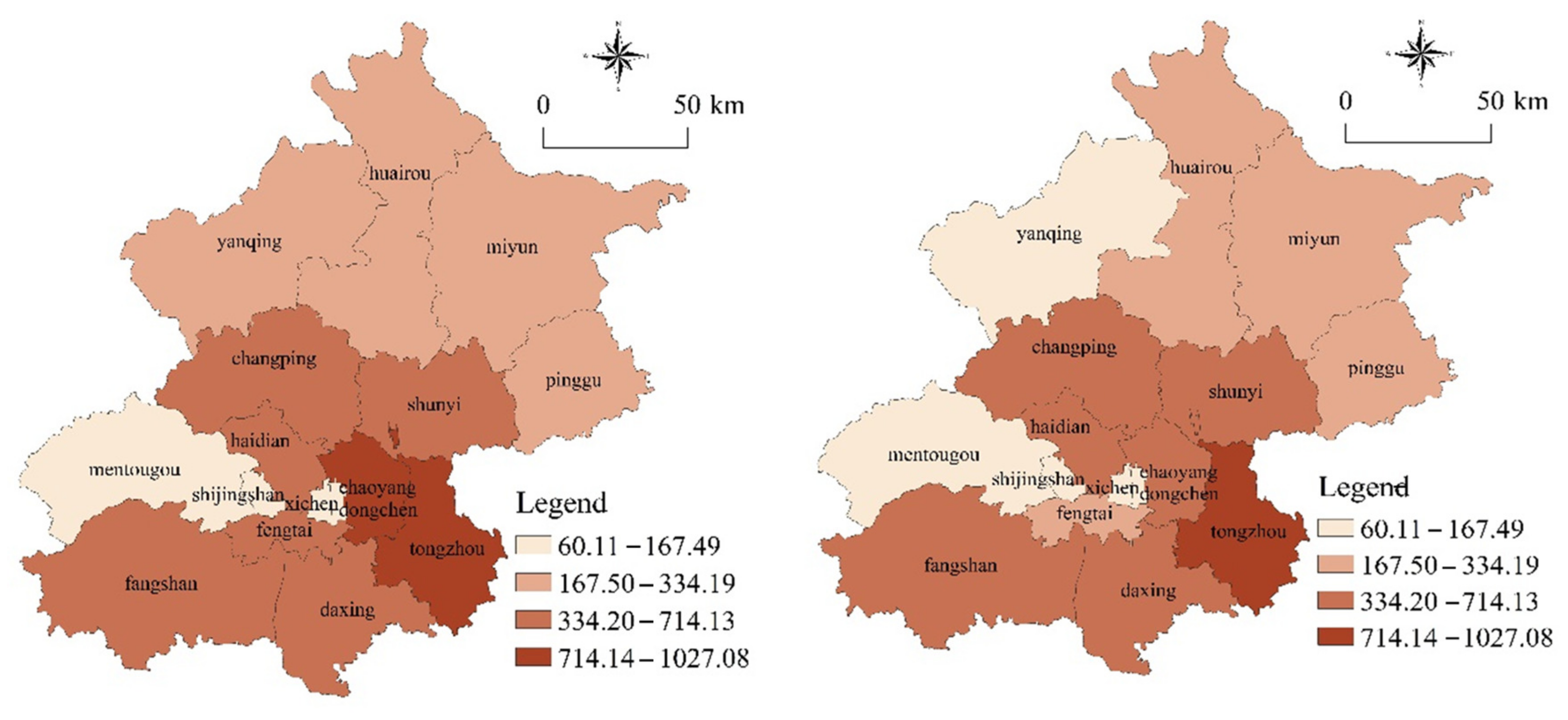
The carbon dioxide emissions of 16 districts in Beijing were calculated. Considering the availability of data, we selected carbon dioxide emissions during the period of 2003 and 2017 to further observe the temporal variation characteristics of carbon dioxide emissions in various districts, as shown in Figure 2. Figure 2 demonstrates that the carbon dioxide emissions in Chaoyang District, Yanqing County, and Fengtai District in 2017 were much lower than those in 2003, indicating the significant progress made in energy saving and emission reduction.

4. Results

4.1. Energy Carbon Emissions and Sectoral Carbon Emissions

As shown in Figure 3, the total carbon dioxide emission in Beijing and the carbon dioxide emission in key departments, including residential, architecture, transportation, and industry, are described.
Figure 3 indicates that carbon dioxide emissions in Beijing showed an earlier increasing and later decreasing trend from 2003 to 2019. Carbon dioxide emissions were about 81.9 million tons in 2003 and increased to 103 million tons in 2010, which shows a high carbon dioxide emission level. After 2010, carbon dioxide emissions gradually declined. In 2019, carbon dioxide emissions were about 85.79 million tons, 16.7% lower than in 2010. Although industrial carbon dioxide emissions have dropped, they still account for a large proportion of the total carbon dioxide emissions. Carbon dioxide emissions from transportation, storage, post, and telecommunication services have continued to rise. Residential and construction carbon dioxide emissions are relatively similar. In 2019, the proportions of industrial, construction, residential, transportation, storage, post, and telecommunication services in total carbon dioxide emissions were 37.96%, 1.23%, 18.12%, and 31.47%, respectively.
The carbon dioxide emissions of agriculture, mining, manufacturing, construction, power, gas, and water production and supply are shown in Figure 4. Since the tertiary industry involves many industries, its comprehensive data are used for descriptive statistics.
The carbon dioxide emissions of agriculture, forestry, animal husbandry, and fisheries have demonstrated relative stability since 2003, making up a modest fraction of Beijing’s overall carbon dioxide emissions. As an essential part of the industrial sector, the carbon dioxide emissions of the mining industry have maintained a relatively low level. They only increased significantly in 2010, with about 8.1 million tons of carbon dioxide emissions, and then gradually decreased. The manufacturing industrial sector’s carbon dioxide emissions were very high in the beginning but have now decreased significantly, by roughly 86.5% in 2019 compared to 2003. The carbon dioxide emissions of the building industry contribute a modest amount of overall emissions, gradually dropping after 2010. In recent years, carbon dioxide emissions from the production and supply of water, gas, and electricity have shown a slow downward trend but still significantly impact Beijing’s total carbon dioxide emissions. In 2019, its carbon emissions accounted for about 33.5% of the total emissions. The carbon dioxide emission of the tertiary industry in Beijing have increased significantly, with an increase of about 21.63 million tons in 2019 compared with 2003. The carbon dioxide emission data of primary, secondary, and tertiary industries can be obtained by classifying each industry into three groups for calculation, as shown in Figure 5.
Following a succession of strategies for changing the industrial structure and energy-saving and emission-reduction initiatives, carbon dioxide emissions from the secondary industry have shown a clear downward trend since 2003, decreasing by about 42% in 2019 compared with 2003. In 2017, the carbon dioxide emissions from the secondary industry were lower than those from the tertiary industry. The proportion of primary industry carbon dioxide emissions in total emissions is relatively small, and its carbon dioxide emissions show a downward trend. The carbon dioxide emissions from the tertiary industry are rising, particularly those generated by the post office, storage, and transportation sectors’ continued growth, which could play a crucial role in future efforts to reduce carbon emissions.

4.2. Carbon Emission Intensity and Per Capita Emission

From 2000 to 2019, Beijing’s energy consumption and CO2 emissions increased at first and then decreased. In 2010, CO2 emissions exceeded 100 million tons. The overall dispersion of the data is low. With the continuous growth of per capita GDP, the growth rate of carbon dioxide emissions is much lower than that of economic development. Beijing has achieved certain results in controlling and reducing coal consumption.
Figure 6 indicates that under the condition that Beijing’s regional GDP increases annually, the carbon emission per unit GDP (CEPUG) decreases year by year. With the growth of Beijing’s overall economic development level, carbon dioxide emission shows a negative correlation change. In 2007, Beijing’s carbon emissions per capita (CEPC) reached an average of 63,000 tons per 10,000 people. The number of permanent residents in Beijing increased yearly from 2003 to 2016 and then decreased. The overall CEPC shows a fluctuating decreasing trend.

4.3. Time Series Dynamic Prediction of Carbon Emissions

4.3.1. CO2 Emission Prediction Results Based on GM (1,1)

Beijing’s carbon dioxide emissions are predicted based on the GM (1,1) model. First, an ex-ante test is performed according to the steps predicted. Since the statistical data are from 2003 to 2019, we define the value of N as 17 to test whether δ belongs to the ( e 2 N + 1 , e 2 N + 1 ) range. The original data column can be predicted by GM (1,1), modeling if the conditions are met. The original data are tested by MATLAB software through the pre-prediction test, and the obtained response function is as follows.
X ( 1 ) ( K + 1 ) = 15844441.1 e 0.0062 K + 1592631.1 .
The average relative error between the initial value obtained after translational transformation and the fitted value is about 3.9%. Then, the trend simulation of the data is performed, as shown in Figure 7. The changes in emissions can be observed more intuitively through the simulation data graph. According to the simulation results, the average growth rate declined after 2004.
The prediction results of the model are also tested accordingly, and the posterior difference test is adopted. The prediction accuracy is comprehensively evaluated according to the comparison between the actual calculation data and the accuracy standard. When P > 0.95 ,   C < 0.35 , the prediction accuracy of the model is high. When 0.8 < P < 0.95 , 0.35 < C < 0.5 , the result is good. When 0.7 < P < 0.8 ,   0.5 < C < 0.65 , the result is qualified. When P < 0.7 , C > 0.65 , the result is unqualified, and the residual can be corrected until the accuracy meets the requirements. According to the test, P = 1, C = 0.58, which meets the prediction accuracy standard, then the carbon dioxide emission of Beijing before 2030 is predicted. Table 1 presents the results.
According to the prediction results, Beijing’s overall carbon dioxide emissions will trend downward in the next few years. Beijing’s carbon dioxide emissions in 2030 are set to be 83.76 million tons, reducing by 2.03 million tons compared with 2019. The actual decline is expected to exceed this estimation through the implementation of a series of emission reduction measures.

4.3.2. CO2 Emission Prediction Based on the BP Neural Network

First, the carbon dioxide emission data of each of the first five years are taken as a training sample by grouping the data. The data of the sixth year are affected by the data of the previous five years. The data from the sixth year are used as a result and divided into groups in turn. Since the first five groups of data are used as training samples, in order to obtain the simulation values from 2003 to 2019, the five-year CO2 emission data from 1998 to 2002 should be added for training, and then 14 groups of sliding time series can be obtained. Next, the data are normalized and processed using MATLAB, and the maximum number of training times is set to 20,000. A comparison chart of the simulated fitted value and the actual value is drawn in order to compare the accuracy of the prediction, as shown in Figure 8. The simulation results show that there is an average absolute error of approximately 338 between the forecast value and the actual figure and an average relative error of 3.9%. The goodness of fit R2 is 0.913, close to 1. The goodness of fit is high, and the prediction results meet the standard.
After data training through BP neural network perceptron, the carbon dioxide emissions before 2030 are predicted, and the data obtained are shown in Table 2. From 2020 to 2030, Beijing’s carbon dioxide emissions will show a fluctuating trend. There will be higher peaks in emissions in 2021, 2024, and 2027, respectively. After 2027, the emissions will show a fluctuating downward trend.

4.3.3. Comparison of CO2 Emission Prediction Results

According to the comparison between the above GM (1,1) model and BP neural network prediction results, both prediction results are scientific to a certain extent, with the same average relative error and good prediction accuracy, which plays an important guiding role in observing the emission characteristics of carbon dioxide in Beijing in the next 10 years and judging whether the carbon neutrality target will be achieved. During the 14th Five Year Plan period, through the implementation of the Action Plan for peaking carbon dioxide emissions, China deeply promoted low-carbon and clean transformation in energy, industry, construction, transportation, and other fields, and vigorously developed non-fossil fuels. Therefore, actual carbon dioxide emissions in the future may be even smaller.
There are also some differences between the results predicted by the two models. It can be seen from Figure 5 and Figure 6 that the GM (1,1) model prediction value is close to the actual value in fewer years, while the BP neural network prediction value is more coincident with the actual value, and its fitting effect is relatively better. The changing trend of prediction results based on the GM (1,1) model is relatively gentle, and the overall emissions showed a downward trend after reaching their peak. The results predicted by the BP neural network vary greatly, showing that carbon dioxide emissions will rise and fall suddenly. From this feature, it can be seen that the GM (1,1) model can be used to predict the change characteristics of carbon dioxide emissions, which can better grasp the overall change trend in the future so as to clarify its emission rules. However, the predicted carbon dioxide emissions have been showing a downward trend in the next few years, and it is impossible to accurately observe the time when carbon emissions become neutral in Beijing. The prediction results of the BP neural network show fluctuating change. The change is relatively slow after reaching a large value in a period. However, the changing trend of overall control of carbon dioxide emissions is relatively weak due to the high frequency of data fluctuation.

4.4. Threshold Model Results

4.4.1. Threshold Result Analysis

Analyzing the driving factors of carbon dioxide emissions is essential for formulating targeted emission reduction measures. This study introduces the extended STIRPAT model to examine the implementation path of carbon reduction from the perspective of key driving forces, such as economic development, natural factors, transportation structure, population size, and technological progress. The threshold regression model is used to examine the relationship between carbon dioxide emissions and the primary driving forces in Beijing. This paper discusses the phased impact of economic development level on carbon dioxide emissions with the change of energy consumption intensity. In the aspect of selecting driving indicators, we refer to the research of Wang et al. [45] and Ma et al. [46] and consider the representativeness and availability of data given the current status of carbon emission characteristics in Beijing. The technical level is selected as the threshold variable, and its specific indicator is energy consumption intensity, represented by ECI. GDP per capita is the core explanatory variable, which is expressed by PCGDP. The index of carbon dioxide emission is the explained variable, represented by CDE. Subsequently, the control variables include the number of permanent residents, the number of civilian vehicles, energy consumption intensity, and the area of urban green space, represented by PR, CV, ECI, and UGS, respectively. According to the above indicators, we conducted a descriptive statistical analysis of the relevant data from 2004 to 2019, as shown in Table 3.
Before analyzing the threshold model, it is necessary to test the threshold effect to determine whether there is a threshold value and its number. Bootstrap was used to repeatedly sample 500 times to improve the efficiency of the threshold effect significance test. This model does not have double or triple threshold values according to a regression test. The threshold test results are significant at the 1% significance level through the single threshold test. The threshold significance test results are shown in Table 4.
The threshold regression model results are shown in Table 5.
According to the regression analysis results, the above results passed the significance test. The factor of per capita GDP has a periodic impact on carbon dioxide emissions under the change in energy consumption intensity. With the improvement of per capita GDP, CO2 emissions will increase. The increase rate will decrease when the logarithm of the value of energy consumption intensity exceeds the threshold value of −0.3769, according to the regression coefficient analysis. Lower energy intensity represents a higher level of technological development. Therefore, in the case of high technological development, the elastic coefficient of the impact of economic development level on carbon dioxide emissions is large. The single factor of technical progress cannot directly control the amount of carbon dioxide emissions, so various factors should be considered.
The results show that the GDP per capita, energy consumption intensity, and the ownership of civil vehicles have a positive impact on carbon dioxide emissions; that is, the increase in the GDP per capita, energy consumption intensity, and the ownership of civil vehicles will increase CO2 emissions. The factors of permanent residents and the area of urban green space have a negative impact on carbon dioxide emissions, which indicates that the increase in population is conducive to the reduction of carbon dioxide emissions. At the same time, the expansion of urban green space has effectively reduced carbon dioxide emissions.

4.4.2. Threshold Model Test

The threshold value can be tested by judging the confidence interval structure of the likelihood ratio statistic (LR) of the threshold variable. LR is the ordinate, and the threshold value of the threshold variable to be estimated is the abscissa. A horizontal dashed line c is drawn to determine the reference confidence level. Among them, α is the significant level, c = 2 l n   ( 1 ( 1 α ) ) . Because of the existence of a single threshold, the confidence level detection charts will be generated by detecting the single threshold value, as shown in Figure 9.
The maximum likelihood ratio is the LR level of the threshold variable. The threshold effect of the threshold variable is present and significant when the LR value of the threshold variable falls inside its 95% confidence interval. The significance of the threshold effect and the number of threshold values (inflection points) are judged by the number and range of LR values of threshold variables falling within their 95% confidence interval. Figure 9 shows that the threshold variable indicator meets the 95% significance level.

4.4.3. Robustness Test

In order to further analyze whether the development of economy and technology has a certain cumulative effect on carbon emissions and weakens the possible endogenous, this study lags behind the core explanatory variables for one year to study its impact on carbon dioxide emissions for a robustness test. The threshold significance test is shown in Table 6.
Table 6 shows that the regression findings are significant and that the threshold value remained constant. Table 7 displays the outcomes of the threshold regression model. The findings indicate that the impact on carbon emissions under the influence of technological level gradually increases as economic development improves. In addition, the elastic coefficient of each control variable has little change. Therefore, it is believed that the impact trend of various variables on carbon dioxide emissions is basically consistent, and the result is robust.

5. Discussion

According to the predicted analysis results, it can be verified that the GM (1,1) model can be used to predict with scanty amounts of imperfect data and be appropriated for data prediction with clear trends. It can be used for short-term forecasting activities. This finding is consistent with previous studies [47]. The BP neural network model can effectively analyze nonlinear data samples by constructing a parallel interconnected network composed of multiple nonlinear simple units. This backpropagation algorithm aims to enhance the connectivity between layers to obtain optimal results [48]. Therefore, it is necessary to combine the BP neural network advantages in nonlinear quantitative analysis of data with the characteristics of the GM (1,1) model of research on carbon emission prediction trends. Based on the two prediction results, the carbon emission prediction trend can be described.
From the regression results in Table 5, it can be seen that Beijing’s carbon dioxide emissions can be reduced in proportion to a decrease in energy intensity. This finding is in line with the studies of Chen et al. [49]. In Beijing, carbon emissions can be reduced by improving the technical level and rationally planning the traffic structure. Similarly, Awan et al. [50] and Sun et al. [51] demonstrated that technological innovation is beneficial for reducing carbon dioxide emissions from a variety of sectors. High-quality economic development can also accelerate the reduction of carbon dioxide emissions, and scientifically expanding the area of urban green space can effectively increase carbon absorption in Beijing. The previous studies indicated that economic development promotes carbon dioxide emissions in selected Sub-Saharan African (SSA) countries [52]. Although their research differs from the regions in this paper, the research results on the impact of economic growth on carbon emissions are similar. Then, the implementation mode of Beijing’s carbon emission reduction path is further explored from the aspect of threshold regression analysis of driving factors. Based on the above discussion, it can be concluded that the relevant research findings are not only applicable to the studied region but also provide a reference for the carbon reduction work of other regions and countries.
The limitations and improvements of this paper are mainly in the following aspects. First, we used the GM (1,1) model to predict carbon emissions. This model predicts current data, easily ignoring new information and failing to consider the impact of more factors. It also has certain requirements for data, which must be positive and have the same time interval. As for further work, we can improve the methods based on actual data to obtain more accurate forecast results. Second, we used data in Beijing for threshold regression analysis. In order to obtain reliable regression results, although we conducted repeated sampling of time series data, there may also be a problem of insufficient sample size. In future research, we can analyze the national data and form panel data for regression to make the research results more reliable. Third, due to the limitations in data availability, the studied factors affecting carbon emissions are limited. Thus, we should further develop and use different indicators in future research to fully analyze the influencing factors of carbon emissions reduction.

6. Conclusions

This study analyzed the carbon dioxide emission characteristics of various departments and three important industries in Beijing. In order to provide references for the analysis of Beijing’s future carbon emission trend, we developed a time series dynamic prediction of the levels of carbon emissions in Beijing before 2030 using the grey GM (1,1) and BP neural network models. Then, the influencing factors of carbon dioxide emissions in Beijing were identified based on the threshold model. The technology level was used as the threshold variable in the study of the relationship between per capita GDP and carbon emissions, and the degree to which each control variable affects carbon emissions was observed. The number of permanent residents and the amount of urban green space had a negative impact on carbon dioxide emissions, while the GDP per capita, energy consumption intensity, and ownership of civil vehicles had positive effects. The carbon emission reduction paths and countermeasures under the carbon neutrality target were discussed based on the analysis of the characteristics and contributing factors of CO2 in Beijing. We proposed several countermeasures and suggestions for Beijing’s implementation of carbon emission reduction measures. Our specific recommendations are as follows:
  • Government departments should further integrate modern service and advanced manufacturing sectors to encourage the upgrading of industrial structures. Beijing should use the tertiary sector to propel the growth of the primary and secondary industries in the future. Regarding primary industries, the government assures the availability of essential agricultural goods and minimizes waste generation and environmental degradation. Enterprises should continue to strive to improve the quality of the secondary industry, enhance the modernization level of industry and supply chain, and pursue the goal of intelligent production and high-end manufacturing.
  • The government should boost carbon emission reduction in the industrial sector while accelerating the development of a high-quality, accurate, and modern economic structure. Beijing should continue to adhere to the direction of intelligent manufacturing and high-end manufacturing and upgrade and transform the energy terminal sector to achieve low-carbon emissions. Subsequently, the regulatory authorities should strictly control the industrial access threshold. Promoting the development of low-carbon technology is also crucial.
  • It is necessary to optimize the transportation structure and implement low-carbon transportation. The carbon emission level of Beijing’s transportation system has been increasing, which is a relatively large emission department after the industrial sector. Therefore, Beijing needs to strengthen the management and control of traffic activities in the process of urbanization, reduce the increase in long-distance traffic activities caused by the expansion of built-up areas, and pay attention to the organic integration of road resources. Furthermore, the government and enterprises should promote the development of transportation energy technology, reduce the energy consumption intensity of urban transportation, and take green transportation as the future development direction.
  • Beijing should implement the green building development strategy and strengthen carbon emission reduction in the construction field. Government departments should improve the qualification standard of green buildings and continue to develop energy-saving technologies. Additionally, Beijing can also establish ultra-low energy consumption buildings, promote near-zero energy consumption buildings, and vigorously develop the recycling of building materials to promote carbon emission reduction through energy conservation.

Author Contributions

Conceptualization, Y.L. and J.D.; methodology, J.D. and H.C.; software, J.D. and S.Z.; validation, Y.L. and H.C.; data curation, J.D. and S.Z.; writing—original draft preparation, J.D.; writing—review and editing, J.D. and H.C.; supervision, Y.L.; project administration, Y.L. All authors have read and agreed to the published version of the manuscript.

Funding

This research was supported by the Key Project of the Beijing Social Science Foundation of China (19YJA002), the Post-funded Project of the National Social Science Foundation of China (21FJYB023), and the Key Project of the Beijing University of Technology for Major Strategic Decision-making Consultation in the Capital in 2022 (011000514122545).

Institutional Review Board Statement

Not applicable.

Informed Consent Statement

Not applicable.

Data Availability Statement

The relevant data used in the study are presented in the data and result section.

Conflicts of Interest

The authors declare no conflict of interest.

References

  1. Shen, Y.; Sun, X.; Fu, Y. The spatial network and its driving factors for sustainable total-factor ecology efficiency: The case of China. Environ. Sci. Pollut. Res. 2021, 28, 68930–68945. [Google Scholar] [CrossRef] [PubMed]
  2. Skytt, T.; Nielsen, S.N.; Jonsson, B.G. Global warming potential and absolute global temperature change potential from carbon dioxide and methane fluxes as indicators of regional sustainability—A case study of Jämtland, Sweden. Ecol. Indic. 2020, 110, 105831. [Google Scholar] [CrossRef]
  3. Yi, S.H.; Xiang, B.; Meng, B.P.; Wu, X.D.; Ding, Y.J. Modeling the carbon dynamics of alpine grassland in the Qinghai-Tibetan Plateau under scenarios of 1.5 and 2 °C global warming. Adv. Clim. Change Res. 2019, 10, 80–91. [Google Scholar] [CrossRef]
  4. Chen, Y.; Liu, S.; Wu, H.; Zhang, X.; Zhou, Q. How can Belt and Road countries contribute to glocal low-carbon development? J. Clean. Prod. 2020, 256, 120717. [Google Scholar] [CrossRef]
  5. Man, Y.; Li, J.; Hong, M.; Han, Y. Energy transition for the low-carbon pulp and paper industry in China. Renew. Sust. Energy Rev. 2020, 131, 109998. [Google Scholar] [CrossRef]
  6. Wei, G.; Bi, M.; Liu, X.; Zhang, Z.; He, B. Investigating the impact of multi-dimensional urbanization and FDI on carbon emissions in the belt and road initiative region: Direct and spillover effects. J. Clean. Prod. 2023, 384, 135608. [Google Scholar] [CrossRef]
  7. Lu, J.; Chen, H.; Cai, X. From global to national scenarios: Exploring carbon emissions to 2050. Energy Strateg. Rev. 2022, 41, 100860. [Google Scholar] [CrossRef]
  8. Xiao, Y.; Ma, D.; Zhang, F.; Zhao, N.; Wang, L.; Guo, Z.; Zhang, J.; An, B.; Xiao, Y. Spatiotemporal differentiation of carbon emission efficiency and influencing factors: From the perspective of 136 countries. Sci. Total Environ. 2023, 879, 163032. [Google Scholar] [CrossRef]
  9. Acheampong, A.O. The impact of de facto globalization on carbon emissions: Evidence from Ghana. Int. Econ. 2022, 170, 156–173. [Google Scholar] [CrossRef]
  10. Bruno, M.; Lopes, D.; Jabbour, C.; Paula, D.; Yusoff, Y.M.; Thomé, A.M.T. Business opportunities and challenges as the two sides of the climate change: Corporate responses and potential implications for big data management towards a low carbon society. J. Clean. Prod. 2018, 189, 763–774. [Google Scholar] [CrossRef]
  11. Gao, J.; Li, G.; Zhang, Y.; Zou, C. Analysis on Goals, Tasks and Realization Path of China’s 14th Five-Year Plan for Ecological and Environmental Protection. Environ. Prot. 2021, 49, 45–51. [Google Scholar]
  12. Tong, Y.; Wang, K.; Liu, J.; Zhang, Y.; Gao, J.; Dan, M.; Yue, T.; Zuo, P.; Zhao, Z. Refined assessment and decomposition analysis of carbon emissions in high-energy intensive industrial sectors in China. Sci. Total Environ. 2023, 872, 162161. [Google Scholar] [CrossRef]
  13. Shen, L.; Wu, Y.; Lou, Y.; Zeng, D.; Shuai, C.; Song, X. What drives the carbon emission in the Chinese cities?—A case of pilot low carbon city of Beijing. J. Clean. Prod. 2018, 174, 343–354. [Google Scholar] [CrossRef]
  14. Zhang, P.; Cai, W.; Yao, M.; Wang, Z.; Yang, L.; Wei, W. Urban carbon emissions associated with electricity consumption in Beijing and the driving factors. Appl. Energy 2020, 275, 115425. [Google Scholar] [CrossRef]
  15. Wang, P.; Huang, R.; Zhang, S.; Liu, X. Pathways of carbon emissions reduction under the water-energy constraint: A case study of Beijing in China. Energy Policy 2023, 173, 113343. [Google Scholar] [CrossRef]
  16. Khalil, A.; Javed, A.; Bashir, H. Evaluation of Carbon Emission Reduction via GCIP Projects: Creating a Better Future for Pakistan. Earth Syst. Environ. 2019, 3, 19–28. [Google Scholar] [CrossRef]
  17. Chhabra, M.; Giri, A.K.; Kumar, A. Do trade openness and institutional quality contribute to carbon emission reduction? Evidence from BRICS countries. Environ. Sci. Pollut. Res. 2023, 30, 50986–51002. [Google Scholar] [CrossRef]
  18. Konstantinaviciute, I.; Bobinaite, V. Comparative analysis of carbon dioxide emission factors for energy industries in European Union countries. Renew. Sust. Energy Rev. 2015, 51, 603–612. [Google Scholar] [CrossRef]
  19. Honma, S.; Ushifusa, Y.; Okamura, S.; Vandercamme, L. Measuring carbon emissions performance of Japan’s metal industry: Energy inputs, agglomeration, and the potential for green recovery reduction. Resour. Policy 2023, 82, 103519. [Google Scholar] [CrossRef]
  20. Gordic, D.; Nikolic, J.; Vukasinovic, V.; Josijevic, M.; Aleksic, A.D. Offsetting carbon emissions from household electricity consumption in Europe. Renew. Sust. Energy Rev. 2023, 175, 113154. [Google Scholar] [CrossRef]
  21. Wu, F.; He, J.; Cai, L.; Du, M.; Huang, M. Accurate multi-objective prediction of CO2 emission performance indexes and industrial structure optimization using multihead attention-based convolutional neural network. J. Environ. Manag. 2023, 337, 117759. [Google Scholar] [CrossRef] [PubMed]
  22. Huang, S.; Xiao, X.; Guo, H. A novel method for carbon emission forecasting based on EKC hypothesis and nonlinear multivariate grey model: Evidence from transportation sector. Environ. Sci. Pollut. Res. 2022, 29, 60687–60711. [Google Scholar] [CrossRef] [PubMed]
  23. Khajavi, H.; Rastgoo, A. Predicting the carbon dioxide emission caused by road transport using a Random Forest (RF) model combined by Meta-Heuristic Algorithms. Sust. Cities Soc. 2023, 93, 104503. [Google Scholar] [CrossRef]
  24. Bai, F.J.J.S. A Machine Learning Approach for Carbon di oxide and Other Emissions Characteristics Prediction in a Low Carbon Biofuel-Hydrogen Dual Fuel Engine. Fuel 2023, 341, 127578. [Google Scholar] [CrossRef]
  25. Maino, C.; Misul, D.; Di Mauro, A.; Spessa, E. A deep neural network based model for the prediction of hybrid electric vehicles carbon dioxide emissions. Energy AI 2021, 5, 100073. [Google Scholar] [CrossRef]
  26. De Oliveira-De Jesus, P.M. Effect of generation capacity factors on carbon emission intensity of electricity of Latin America & the Caribbean, a temporal IDA-LMDI analysis. Renew. Sust. Energy Rev. 2019, 101, 516–526. [Google Scholar] [CrossRef]
  27. Wang, Z.; Xie, W.; Zhang, C. Towards COP26 targets: Characteristics and influencing factors of spatial correlation network structure on US carbon emission. Resour. Policy 2023, 81, 103285. [Google Scholar] [CrossRef]
  28. Bezuglov, A.; Comert, G. Short-term freeway traffic parameter prediction: Application of grey system theory models. Expert Syst. Appl. 2016, 62, 284–292. [Google Scholar] [CrossRef]
  29. Guefano, S.; Tamba, J.G.; Azong, T.E.W.; Monkam, L. Methodology for forecasting electricity consumption by Grey and Vector autoregressive models. MethodsX 2021, 8, 101296. [Google Scholar] [CrossRef]
  30. Kayacan, E.; Ulutas, B.; Kaynak, O. Grey system theory-based models in time series prediction. Expert Syst. Appl. 2010, 37, 1784–1789. [Google Scholar] [CrossRef]
  31. Khan, A.M.; Osińska, M. Comparing forecasting accuracy of selected grey and time series models based on energy consumption in Brazil and India. Expert Syst. Appl. 2023, 212, 118840. [Google Scholar] [CrossRef]
  32. Kazancoglu, Y.; Ozbiltekin-Pala, M.; Ozkan-Ozen, Y.D. Prediction and evaluation of greenhouse gas emissions for sustainable road transport within Europe. Sust. Cities Soc. 2021, 70, 102924. [Google Scholar] [CrossRef]
  33. Saxena, A. Grey forecasting models based on internal optimization for Novel Corona virus (COVID-19). Appl. Soft Comput. 2021, 111, 107735. [Google Scholar] [CrossRef]
  34. Pai, T.Y.; Ho, C.L.; Chen, S.W.; Lo, H.M.; Sung, P.J.; Lin, S.W.; Lai, W.J.; Tseng, S.C.; Ciou, S.P.; Kuo, J.L.; et al. Using seven types of GM (1, 1) model to forecast hourly particulate matter concentration in Banciao city of Taiwan. Water Air. Soil Pollut. 2010, 217, 25–33. [Google Scholar] [CrossRef]
  35. Soleimani, L.F.; Khorrami, M.K.; Zandbaaf, S.; Bardajee, G.R.; Noor, P.; Ghasemi, K. Determination of micropore volumes of ZSM-5 zeolite samples by diffuse reflectance infrared Fourier transform (DRIFT) spectroscopy using back-propagation artificial neural network (BP-ANN) and non-negative matrix factorization-alternating least squares (NMF-ALS) as chemometric approaches. Infrared Phys. Technol. 2020, 111, 103543. [Google Scholar] [CrossRef]
  36. Cui, Z.Q.; Wang, C.H.; Gao, X.H.; Tian, S.S. State of health estimation for lithium-ion battery based on the coupling-loop nonlinear autoregressive with exogenous inputs neural network. Electrochim. Acta 2021, 393, 139047. [Google Scholar] [CrossRef]
  37. Xue, W. Construction of low carbon city economic security management system based on BP artificial neural network. Sustain. Energy Technol. Assess. 2022, 53, 102699. [Google Scholar] [CrossRef]
  38. Wang, Y.; Li, K.Q.; Zeng, X.H.; Gao, B.L.; Hong, J.C. Energy consumption characteristics based driving conditions construction and prediction for hybrid electric buses energy management. Energy 2022, 245, 123189. [Google Scholar] [CrossRef]
  39. Rumelhart, D.E.; Mcclelland, J.L. The Appeal of Parallel Distributed Processing; MIT Press: Cambridge, MA, USA, 1987. [Google Scholar]
  40. Ehrlich, P.R.; Holdren, J.P. Impact of Population Growth. Science 1971, 171, 1212–1217. [Google Scholar] [CrossRef]
  41. Richard, Y.; Eugene, A.R.; Thomas, D. STIRPAT, IPAT and ImPACT: Analytic tools for unpacking the driving forces of environmental impacts. Ecol. Econ. 2003, 46, 351–365. [Google Scholar] [CrossRef]
  42. Hansen, B.E. Threshold effects in non-dynamic panels: Estimation, testing, and inference. J. Econ. 1999, 93, 345–368. [Google Scholar] [CrossRef]
  43. Guan, Y.; Shan, Y.; Huang, Q.; Chen, H.; Wang, D.; Hubacek, K. Assessment to China’s recent emission pattern shifts. Earth Future 2021, 9, e2021EF002241. [Google Scholar] [CrossRef]
  44. Shan, Y.; Huang, Q.; Guan, D.; Hubacek, K. China CO2 emission accounts 2016–2017. Sci. Data 2020, 7, 54. [Google Scholar] [CrossRef] [PubMed]
  45. Wang, Y.; Xu, Z.Y.; Zhang, Y.X. Influencing factors and combined scenario prediction of carbon emission peaks in megacities in China: Based on Threshold—STIRPAT Model. Acta Sci. Circumst. 2019, 39, 4284–4292. [Google Scholar]
  46. Ma, X.; Wang, C.; Dong, B.; Gu, G.; Chen, R.; Li, Y.; Zou, H.; Zhang, W.; Li, Q. Carbon emissions from energy consumption in China: Its measurement and driving factors. Sci. Total Environ. 2019, 648, 1411–1420. [Google Scholar] [CrossRef]
  47. Ceylan, Z.; Bulkan, S.; Elevli, S. Prediction of medical waste generation using SVR, GM (1,1) and ARIMA models: A case study for megacity Istanbul. J. Environ. Health Sci. Eng. 2020, 18, 687–697. [Google Scholar] [CrossRef]
  48. Amin, S. Backpropagation–artificial neural network (BP-ann): Understanding gender characteristics of older driver accidents in west midlands of United Kingdom. Saf. Sci. 2020, 122, 104539. [Google Scholar] [CrossRef]
  49. Zhu, C.; Chang, Y.; Li, X.; Shan, M. Factors influencing embodied carbon emissions of China’s building sector: An analysis based on extended STIRPAT modeling. Energy Build. 2022, 255, 111607. [Google Scholar] [CrossRef]
  50. Sun, Y.; Hao, S.; Long, X. A study on the measurement and influencing factors of carbon emissions in China’s construction sector. Build. Environ. 2023, 229, 109912. [Google Scholar] [CrossRef]
  51. Awan, A.; Alnour, M.; Jahanger, A.; Onwe, J.C. Do technological innovation and urbanization mitigate carbon dioxide emissions from the transport sector? Technol. Soc. 2022, 71, 102128. [Google Scholar] [CrossRef]
  52. Alaganthiran, J.R.; Anaba, M.I. The effects of economic growth on carbon dioxide emissions in selected Sub-Saharan African (SSA) countries. Heliyon 2022, 8, e11193. [Google Scholar] [CrossRef]
Figure 1. Structure of BP neural network prediction model.
Atmosphere 14 00798 g001
Figure 2. Distribution map of carbon dioxide emissions in Beijing in 2003 (left) and 2017 (right).
Atmosphere 14 00798 g002
Figure 3. Total carbon dioxide emissions and carbon dioxide emissions of key industries.
Atmosphere 14 00798 g003
Figure 4. Carbon emissions of various industries.
Atmosphere 14 00798 g004
Figure 5. Changing trend of carbon emissions of various industries.
Atmosphere 14 00798 g005
Figure 6. Carbon emissions per capita (Unit: tons/person) and per unit GDP (Unit: Ton/104 yuan).
Atmosphere 14 00798 g006
Figure 7. Comparison of simulated data with actual data.
Atmosphere 14 00798 g007
Figure 8. Comparison between actual values and predicted values based on BP neural network.
Atmosphere 14 00798 g008
Figure 9. Test of threshold value.
Atmosphere 14 00798 g009
Table 1. Predicted emission of CO2 in Beijing (unit: 104 tons).
YearPredicted ValueYearPredicted Value
2020891620268588
2021886020278535
2022880520288482
2023875020298429
2024869620308376
20258642
Table 2. Predicted emissions of CO2 (unit: 104 tons).
YearPredicted ValueYearPredicted Value
2020887120269712
202110,327202710,089
2022904520289142
2023961120299867
202410,60220309526
20258870
Table 3. Descriptive statistics of variables.
VariableUnitMEANS.D.MinMax
Carbon dioxide emissions (CED)104 tons9405565849710,300
Energy consumption intensity (ECI)tons of standard coal0.490.240.231.03
GDP per capita (PCGDP)yuan89,76337,08341,099164,000
Permanent population (PR)104 persons194224914932173
Civil car ownership (CV)104 vehicles460132229.6608.4
Urban green space (UGS)104 hectares6.561.524.448.87
Data source: Beijing Statistical Yearbook (2005–2020), China Urban Statistical Yearbook (2005–2020).
Table 4. Threshold value test (a).
ThresholdRSSMSEFPThreshold Value
Single0.01940.000667.15 ***0.00−0.3769
Note: *** mean significant at 1% significance levels.
Table 5. Threshold regression results (a).
VariablesParameters
Ln PR−0.204 ***
Ln CV0.254 ***
Ln ECI0.387 ***
Ln UGS−0.083 ***
ln PCGDP (ln ECI ≤ −0.3769)0.189 ***
ln PCGDP (ln ECI > −0.3769)0.173 ***
Constant7.495 ***
R-squared0.881
*** p < 0.01.
Table 6. Threshold value test (b).
ThresholdRSSMSEFPThreshold Value
Single0.02000.000744.05 ***0.00−0.3769
Note: *** mean significant at 1% significance levels.
Table 7. Threshold regression results (b).
VariablesParameters
Ln PR−0.196 ***
Ln CV0.233 ***
Ln ECI0.277 ***
Ln UGS−0.052 ***
ln PCGDP (ln ECI ≤ −0.3769)0.066 ***
ln PCGDP (ln ECI > −0.3769)0.053 ***
Constant8.813 ***
R-squared0.8665
*** p < 0.01.
Disclaimer/Publisher’s Note: The statements, opinions and data contained in all publications are solely those of the individual author(s) and contributor(s) and not of MDPI and/or the editor(s). MDPI and/or the editor(s) disclaim responsibility for any injury to people or property resulting from any ideas, methods, instructions or products referred to in the content.

