Article

Semiempirical Models of Speedup Effect for Downburst Wind Field over 3-D Hills

Chongqing Key Laboratory of Wind Engineering and Wind Resource Utilization, Chongqing University, Chongqing 400044, China
*
Author to whom correspondence should be addressed.
Atmosphere 2023, 14(4), 694; https://doi.org/10.3390/atmos14040694
Submission received: 9 February 2023 / Revised: 30 March 2023 / Accepted: 4 April 2023 / Published: 7 April 2023
(This article belongs to the Special Issue Advances in Computational Wind Engineering and Wind Energy)

Abstract

:
Downbursts occur frequently in mountainous regions, such as the southwest of China, and causing extensive damage to engineering structures. While some researchers have developed semiempirical models for the speedup effect, most are based on the wind field in the boundary layer over the hill, and there is a lack of semiempirical models for the downburst wind field over the hill. This study employs three RANS (Reynolds Average Navier-Stokes) turbulence models to numerically simulate the downburst wind field over a quadratic curved hill. The realizable k-ε model is selected as the optimal model for the subsequent numerical simulations based on comparison with wind tunnel test results. Then, a semiempirical model of the speedup effect of the downburst wind field over the hill is constructed by numerically simulating the downburst wind field over the hill with different radial locations and different slopes. Finally, the constructed semiempirical model is validated and demonstrates good accuracy.

1. Introduction

When downbursts impact the ground, airflow spreads around the surrounding area [1]. In this process, catastrophic winds possessing a significant destructive force are generated, resulting in potential severe wind damage to engineering structures such as buildings and transmission line towers [2,3,4]. The load values specified in China’s existing load code [5] are determined by the wind field of the atmospheric boundary layer (ABL). The wind characteristics of downbursts are considerably distinct from those of the ABL wind field. Consequently, the study of the wind characteristics of downbursts holds substantial practical significance.
Downbursts mostly occur in mountainous and hilly areas, where the topography exerts a considerable influence on the near-surface wind field. Some researchers have validated these findings by conducting microscale and mesoscale numerical simulations. Homar et al. [6] analyzed intense convective weather in Spain in 1999 and pointed out that the complex mountainous terrain can significantly enhance the destructiveness of storms. Wang Q et al. [7,8,9] emphasized that the wind field environment in complex terrain is intricate and requires a mesoscale model to analyze wind resource data comprehensively for investigating wind farm wake flow. Furthermore, they investigated the impact of atmospheric stability on wind farms located in complex terrain. The objective of this study is to develop a model for downburst wind fields over hilly terrain, assuming neutral conditions. Therefore, the interference effect of terrain on the downbursts is also of interest.
Selvam and Holmes [10] conducted a study of downburst wind fields over a single hill with a slope of 0.25 using the impinging jet model and Computational Fluid Dynamics (CFD) simulations. Their research concluded that the wind speed at the top of the hill under the downburst wind field was lower compared to that under the boundary layer wind field. Letchford and Illidge [11] conducted numerical simulations to investigate the hilltop speedup factor of a cosine-shaped hill and escarpment by varying the slope and radial distance. The results demonstrated that the hilltop speedup factor is directly proportional to the hill’s slope and inversely proportional to the radial distance increase. Mason et al. [12] utilized the cooling source method to investigate the downburst wind field over the escarpment, triangular hill, and bell-shaped hill. The study obtained characteristics of the downburst wind field by varying parameters such as the slope, radial position, and diameter of the downburst. While many researchers [13,14,15,16] have studied downburst wind characteristics over real topography, applying their findings to wind resistance design remains challenging. Thus, it is increasingly apparent that semiempirical models are necessary for the wind-resistant design of structures. These models can simplify and directly describe downburst wind profiles. Despite the complex nature of downburst wind characteristics and the incomplete understanding of their dynamics, simplified semiempirical models provide valuable tools for wind resistance design in regions where downbursts are a dominant extreme wind.
There have been several semiempirical models proposed to study wind fields influenced by hills under the boundary layer. Jackson and Hunt [17] proposed an analytical algorithm to study speedup effects in mountains under the boundary layer, based on two-dimensional hills. They proposed a linear theory of neutrally stratified turbulence on hills. Taylor [18] proposed a simplified algorithm that can consider the effects of different heights of hills. Weng and Taylor [19] investigated the impact of mountain dimension and ground roughness on the speedup ratio using the boundary layer numerical simulation program MSFD (mixed spectral finite difference). They proposed an algorithm for the hilltop speedup ratio that can consider the effect of ground roughness. There are also many research results in constructing semiempirical models of downbursts in flat terrain. Osegura and Bowles [20] proposed a three-dimensional downburst wind speed model, referred to as the OB model, representing that two directional components of downburst wind speed are mainly expressed using horizontal or vertical shape functions. Based on the OB model, Vicroy [21] improved the horizontal and vertical shape functions of the horizontal wind speed and modified the model, referred to as the OBV model. Holmes and Oliver [22] proposed a radial wind profile expression for the horizontal component of mean wind speed, which mainly considers the radial distance from the impinging jet nozzle and the transit time of the downburst, referred to as the Holmes model. The Holmes model was proposed based on experimental and numerical simulations and was limited to the horizontal wind speed profile. Based on the OBV model and Holmes model, Li et al. [23] combined with the measured mean wind speed from Hjelmfelt [24] and the results of CFD simulations, redefined the parameters of shape functions and introduced the maximum horizontal wind speed as a function of radial position and vertical position into the empirical model, i.e., the development of boundary layer nonlinearity was considered, referred to as the Li model. The Li model can simulate the horizontal wind speed considering the nonlinear development of the wind field and shows promising results.
Downburst wind fields over hilly and mountainous terrain have been extensively studied by researchers. Likewise, semiempirical models for downburst wind fields over flat terrain have also been the subject of numerous investigations. However, the development of additional semiempirical models that account for the speedup effect of downburst wind fields over hills remains necessary. This paper aims to construct and verify such models through numerical simulations, which consider different slopes and radial distances. Ultimately, this research will provide some reference for the future construction of speedup ratio models for complex terrain impacted by downbursts.
Section 2 mainly introduces the overview of numerical simulation. In addition, the wind tunnel tests verify the accuracy of numerical simulation. In Section 3, the speedup ratio model is constructed based on the hill’s radial distance, the hill’s slope, and the height above the ground. The paper concludes with Section 4.

2. Numerical Simulations

This section begins with a concise overview of three RANS models and their computational settings. Next, numerical results from these turbulence models are compared quantitatively and qualitatively with wind tunnel test results to verify the reliability of the simulations. Finally, the section presents the settings for various computational cases, which primarily focus on specifying the different slopes and radial positions of hills.

2.1. Flowchart for Numerical Simulations

To demonstrate better the methodology of numerical simulations in this paper, the corresponding flowchart is given in Figure 1.

2.2. RANS Models

The RANS model is the most commonly used numerical simulation method due to its fast computational speed and low cost. The basic idea behind this method is to avoid direct solution of the transient Navier–Stokes (N–S) equation. Instead, the transient N–S equation is averaged using statistical turbulence theory, and the transient velocity is decomposed into its average and fluctuating components. By employing the Boussinesq assumption [25] for the unsteady N–S equations, the governing equations of the RANS model can be expressed as:
u i ¯ x i = 0
ρ u i ¯ t + ( ρ u i u j ¯ ) x i = p ¯ x i + τ i j x j + x j μ u i ¯ x j
where ρ is the fluid density, u i ¯ is the velocity vector, μ is turbulence viscosity, and τ i j = ρ u i u j ¯ is Reynolds stress.
In this study, the RNG k-ε, Realizable k-ε (REA k-ε), and SST k-ω models were chosen to study the flow characteristics of downbursts over the hill. The RNG k-ε model, proposed by Yakhot and Orzag [26], includes an additional term in the input equation to improve the accuracy of fast strain flows, and analytically derives a differential formulation for effective viscosity to account for low Reynolds number effects. The REA k-ε model, proposed by Tsan-Hsing et al. [27], includes alternative equations for turbulent viscosity and a modified transport equation for the dissipation rate ε based on the mean square value transport equation for the vortex pulsation. Compared to the standard k-ε model, the REA k-ε model has a broader range of applications and enables accurate predictions in simulations with large curvature walls, inverse pressure gradients, and flow separation, and can simulate rotation, separation, and secondary flow. The SST k-ω model, improved by Menter [28], revises the definition of turbulent viscosity and takes into account the transport of the main turbulent shear stress. It can solve the standard turbulent kinetic energy equation and the equation of specific turbulence rate, with high accuracy in simulating flows featuring separation, wall jets, and curvature.

2.3. Computational Settings

In this paper, a three-dimensional computational domain was established for numerical simulations using a geometric scale ratio of 1:1000. Figure 2a shows the computational domain, with a quadratic curve-shaped hill as the model in the simulation. The hill model is determined using Equation (3), where z represents the local elevation of the topographic feature, h represents the hilltop height, L represents the maximum radius of the hill in the horizontal direction, and x and y represent the radial distance in the horizontal direction to the hilltop on the x and y-axis, respectively. Additionally, the topographic slope is defined by Equation (4).
z = h ( ( x 2 + y 2 ) L 2 + 1 )
ϕ = h L
Due to the high computational cost of the overall modeling, only one-fourth of the cylinder was used instead of the entire computational domain. The validity of using a partial cylindrical domain instead of the full cylindrical domain was confirmed by Li et al. [20] and Abd-Elaal et al. [10]. In addition, the downburst diameter is Djet = 600 mm, the radial distance from the jet centre line to the outlet side is 7.0 Djet, and the jet height is equal to 1.0 Djet. The hill model is placed at radial distances (refer to r in Figure 2) 1.0 Djet to 2.0 Djet from the jet centre line. The velocity inlet boundary is set at an input wind speed of uj = 10 m/s for the entrance of the computational domain. The outlet applies a pressure boundary condition with a zero gradient for both velocity and pressure in the downstream direction. The side and top surfaces of the computational domain adopt symmetric boundaries. Additionally, the ground uses a no-slip wall boundary condition with zero velocity components and normal pressure gradients for all velocities.
The grid layout is shown in Figure 2b, and the grid in the near-wall region of the hill model is refined to accurately capture the complex turbulent characteristics of the flow field around the hill. In areas with large wind speed gradients, such as the near wall surface and wake area of the hill model, the size of adjacent grids should be similar to minimize numerical truncation error. Through grid-independent analysis, the first layer grid is considered as 0.002 m, the grid growing ratio is 1.05, and the total number of grids is 5.6 × 10⁶.
For all the numerical simulations in this study, the SIMPLE (Semi-Implicit Method for Pressure-Linkage Equations) algorithm is used for the pressure–velocity coupling. Second-order discretization schemes are used for both the convection terms and the viscous terms of the governing equations.

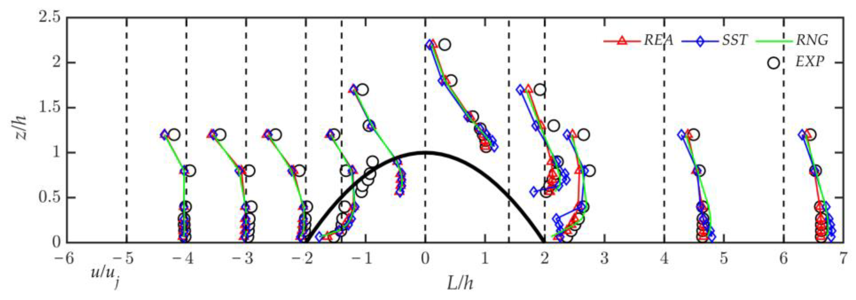
2.4. Verification of Numerical Simulations

An impinging jet test was conducted at the Laboratory of Structural Wind Engineering and Urban Wind Environment of Beijing Jiaotong University to verify the numerical simulation. The impinging jet device is shown in Figure 3. The outlet diameter of the downburst simulator is Djet = 600 mm, the outlet height in this experiment is H = 1.0 Djet, and the outlet wind speed is 10 m/s. Figure 3b shows the arrangement of measuring points. There are 9 measurement points along the horizontal direction with x = −4h, −3h, −2h, −1.4h, 0, 1.4h, 2h, 4h, and 6h. In addition, there are 7 measurement points arranged along the vertical direction, namely z = 5 mm, 10 mm, 15 mm, 20 mm, 30 mm, 60 mm, and 90 mm, respectively.
Three RANS turbulence models, including the REA k-ε, RNG k-ε, and SST k-ω, are used to perform numerical simulations with the identical settings, respectively. Figure 4 compares the numerical simulation results and the wind tunnel test results of the impinging jet. The distribution trends of the two sets of numerical results are the same. In the windward position of the hill, the simulated wind velocities are generally consistent with the measured values. At the foot of the hill, each of the three turbulence models underestimates the wind speed at the near-wall position. At the leeward hillside, each of the three turbulence models overestimate the wind speed near the surface. The test results differ significantly from the wind speed on the leeward hillside since the return flow cannot be measured. At the leeward foothill location, the results of the REA k-ε model are in good agreement with the experimental near-wall wind speeds.
To quantify the accuracy of the results for different turbulence models, Table 1 shows the percentage of differences between simulated and experimental values less than 10%, 20%, and 30% and the Mean Normalized Bias (MNB) [29], where MNB represents the mean relative error between simulated and experimental values, defined as follows.
M N B = 1 N i = 1 N ( V i , f i t t i n g V i , exp ) V i , exp
where N is the number of wind speed measurement points in the test, and Vi,exp, and Vi,fitting are the wind speed values obtained from the test and simulation, respectively.
MNB provides a comprehensive correlation analysis. A negative MNB value indicates that the simulated values are overall smaller than the experimental values, and vice versa. Upon error analysis, the error percentage for the REA k-ε model falls outside the 30% confidence interval by a significant margin (more than 85%). As a result, the REA k-ε model outperforms other RANS models and has been selected for subsequent numerical simulations.

2.5. Arrangement of Different Hill Models

To investigate the effect of hill slope, the study compared eight models of hills with quadratic curves, as listed in Table 2. For example, the Quad-L500-H075 model is a quadratic curve-shaped hill with a maximum base radius of 500 mm and a height from the base to the highest point of 75 mm. These models were positioned at a radial distance of 1.5 times the diameter of the jet. The aim of using these models was to examine their influence on the system’s outcome.
To examine how the speedup ratio varies with the radial position of the hill within the computational domain, the study selected the Quad-L150-H075 model and placed it at various radial distances. Specifically, the hill was positioned at 1.0 Djet, 1.1 Djet, 1.2 Djet, 1.3 Djet, 1.4 Djet, 1.5 Djet, 1.6 Djet, 1.7 Djet, 1.8 Djet, 1.9 Djet, and 2.0 Djet.

3. Semiempirical Model of Speedup Effect for Downburst over the Hill

This section presents and validates semiempirical speedup models for downbursts over hills with varying slopes and radial distances.
To measure the “fractional speedup ratio” [14], one common test of any model, whether analytic or numerical, is to define the following speedup ratio—the ratio of the flow velocity at a certain height above the hilltop to the free-flow velocity at the same height. For clarity, in the following text, this ratio will be referred to as the “speedup ratio”.
Δ S = u ( x , Z ) u f ( Z ) u f ( Z )
where u ( x , Z ) is the velocity measured at a specified elevation, Z = z z h , above a topographical feature. Similarly u f ( Z ) is the velocity measured at the same radial location and elevation with no topography. z h = h ( x ) is the height of the mountain corresponding to the x-axis.

3.1. Modeling Based on the Radial Position of the Hill

The study aimed to explore the speedup effect of placing the Quad-L150-H075 hill model at different radial positions. Figure 5a displays the speedup ratio at the foothill of the windward side, with a maximum absolute value that can reach 0.8. This indicates a significant deceleration effect. As the vertical height increases, the speedup ratio also increases, resulting in a speedup effect. This trend is attributed to a smaller wind speed on flat terrain at this location. Conversely, at r/Djet = 1.0, the speedup ratio increases only slightly with increasing vertical height, while significant deceleration effects occur at the near ground. Figure 5b shows the speedup ratio at the foothill of the leeward side, which exhibits pronounced deceleration effects at all hill positions and a maximum absolute value of 0.9 at r/Djet = 1.0. Near to the ground, the speedup ratio increases with increasing radial distance. Figure 5c illustrates the speedup ratio at the hilltop, which maximum value occurs at near-ground height around radial position 1.5 Djet. When the radial position is before 1.5 Djet, the speedup ratio is similar at the near-ground position. Conversely, the speedup ratio decreases with radial distance as the wind speed is smaller on flat terrain at radial position 1.5 Djet~2.0 Djet. The speedup ratio decays faster when the radial position is closer to the impinging jet center at increasing vertical height.
Figure 6 shows the distribution of the speedup ratio along the vertical height direction at different radial distances at the hilltop. The speedup ratio reaches its maximum value at the near-ground position, with no change in the near-ground speedup ratio observed at radial distances less than 1.5 Djet position. The speedup ratio decreases with the increase of radial distance at the radial distance greater than 1.5 Djet. This relationship can be attributed to the larger radial distance and the larger decreasing gradient of velocity along the height in the downbursts.
For hills with the same slope in the fully developed region of the jet, the corresponding flow separation would be the same and, correspondingly, the speedup ratio distribution along the hill model should also be the same. Figure 7 compares the distribution of the speedup ratio values along the windward side of the hill for near-surface heights of Z/h = 0.0133, Z/h = 0.067, and Z/h = 0.133, using the same slope of the hill model.
Figure 7a shows the speedup at radial distances of 1.2 Djet, 1.5 Djet, and 1.8 Djet for three vertical heights: Z/h = 0.0133, Z/h = 0.067, and Z/h = 0.133. At each height, the speedup ratios for each radial distance are similar. Figure 7b shows the dimensionless distribution of the speedup ratio at each height. On the windward side, the maximum value of the speedup ratio is used as a reference. As seen in Figure 7, the highest speedup ratio occurs between 0.7h and 0.9h on the windward side, rather than at the hilltop. The trend of the dimensionless speedup ratio at each radial distance is consistent across different heights, and the dimensionless distribution of the speedup ratio can be described by Equation (7).
Δ S W + 1 Δ S max + 1 = 0.998 exp ( z h h 0.83 ) 2 0.81
where ΔSW is the speedup ratio at each position on the windward side of the hill, and ΔSmax is the maximum speedup ratio at the windward side of the hill.
Figure 8 illustrates the distribution of the speedup ratio values on the leeward side of the hill at various radial distances with respect to changes in downstream distance. According to Figure 8a, at the same elevation level, the speedup ratio values on the leeward side of the hill reach the maximum value at the hilltop for each radial distance, and the speedup ratio values at each radial distance exhibit a linear correlation with the downstream distance. Furthermore, based on Figure 8b, the trend of the speedup ratio at different radial distances changes in the same pattern concerning the downstream distance, with approximately equivalent slopes. Therefore, the maximum speedup ratio can be normalized, and the hilltop speedup ratio can be used to express the speedup ratio values at different positions in the hill model; the distribution of speedup ratio values along the hill model can be represented by Equation (8).
Δ S L + 1 Δ S T + 1 = 0.73 z h h + 0.22
where ΔSL is the speedup ratio at each location on the leeward side of the hill, and ΔST is the speedup ratio at the hilltop.
The speedup ratios at different radial distances along the windward and leeward sides were obtained from Equations (7) and (8), respectively. The hilltop speedup ratio variation with radial distance was determined from these ratios. The speedup ratio distribution of the hill model at different radial positions was then obtained. Figure 9 displays the variation of the hilltop position speedup ratio with radial distance at the near ground position (Z/h = 0.0133). Before 1.5 Djet, the speedup ratio remained relatively constant with increasing radial distance, but after 1.5 Djet, the speedup ratio decreased more rapidly. The equation for the hilltop speedup ratio variation with radial distance is presented below.
Δ S T r = 0.489 ( r D j e t ) 2 1.2 ( r D j e t ) + 1   r D j e t 1.5 1.5 ( r D j e t ) 2 5.6 ( r D j e t ) + 5.31 r D j e t > 1.5
where ΔSTr is the hilltop speedup ratio at different radial positions.

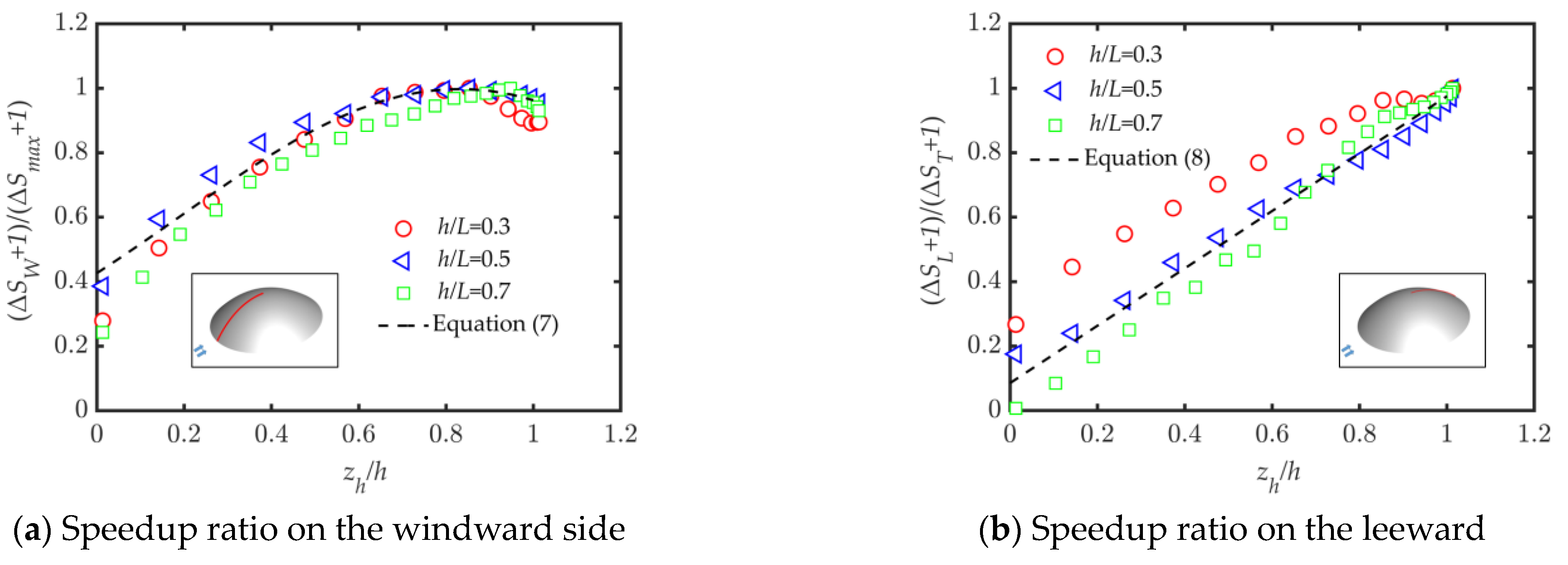
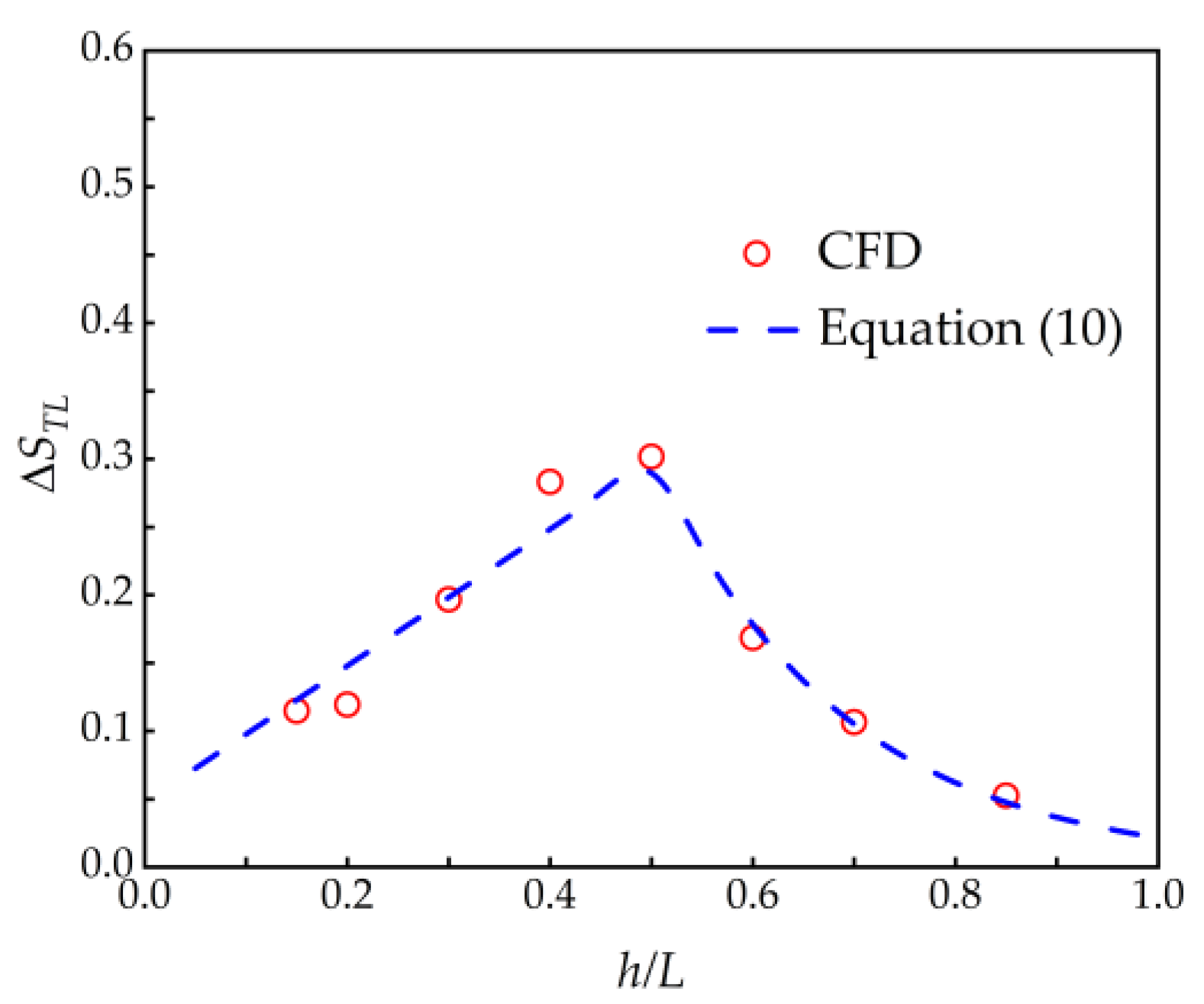
3.2. Modeling Based on the Hill Slopes

Section 3.2 discusses the speedup ratio equations for the windward and leeward sides of the hill, as well as the near-ground hilltop for different radial distances with a slope of 0.5. Next, hills with varying slopes are numerically simulated and analyzed at a 1.5 Djet radial position.
Figure 10 illustrates the speedup ratios at the windward foothill, leeward foothill, and hilltop for different slopes. In Figure 10a, the speedup ratios of the windward foothills are all negative at the near-ground position, increasing in absolute value with the increase in slope. The deceleration effect is significant at a slope of 0.6, and then the speedup ratio decreases with further increases in slope. The speedup ratio at the leeward side is the same as that at the foothill of the windward side, with its absolute value reaching maximum at a slope of 0.6, nearly 1.0, as shown in Figure 10b. Figure 10c displays the maximum speedup ratio of the hill, which reaches approximately 0.35. The speedup ratio increases initially and then decreases in response to the increasing slope.
From the investigation above, it can be noted that in the hill model the speedup ratio at the hilltop position is the maximum value, so the speedup ratio at the hilltop position at different slopes is selected for the study. As shown in Figure 11, at near-ground locations on the hilltop, the speedup ratio increases and then decreases with the increase of the hill slope at each height of the hilltop, and the speedup ratio reaches the maximum value of 0.35 at the slope of 0.5. The reason for this phenomenon is that the nonconfined nature of the wall jet does not allow for a quick reattachment of the separated flow, which is consistent with Mason et al. [9]. The speedup ratio decreases with the increase in the vertical height at each slope and reaches the maximum speedup ratio at the position near the ground. Since the distribution trend of the speedup ratio along the hill is similar at each vertical height, the trend of the speedup ratio at each position along the windward and leeward sides of the hill is studied by selecting the near-ground position (Z/h = 0.0133) to provide a basis for building the speedup ratio model for hilly terrain.
Figure 12 shows the trend of the distribution of speedup ratios along the windward and leeward sides of the hill model for slopes of 0.3, 0.5, and 0.7, respectively. Figure 12a shows the results of dimensionless processing of the speedup ratio on the windward side of the hill model at different slopes with the maximum speedup ratio value. The comparison with Equation (7) shows the same trend, so it can be considered that the speedup ratio on the windward side at different slopes can be expressed by using Equation (7). Figure 12b shows the dimensionless speedup ratios on the leeward side at different slopes and, compared with Equation (8), it is found that the agreement is better, so Equation (8) can express the speedup ratios at different slopes.
The variation of the speedup ratio at the hilltop with slope is shown in Figure 13. When the slope is less than 0.5, the speedup ratio at each position increases linearly with the increase in slope. When the slope is greater than 0.5, the speedup ratio decays in a quadratic curve shape with the increase of slope. The specific expression is shown in Equation (10).
Δ S T L = h L × 0.502 + 0.047 h L 0.5 4.182 exp 5.278 ( h L ) h L > 0.5
where ΔSTL is the speedup ratio at the hilltop for different slopes.
Equation (10) is the speedup ratio of the hilltop at the radial position 1.5 Djet under different slopes. The speedup ratio of the hilltop at different radial distances under any slope can be obtained by combining Equation (9), and the maximum speedup ratio on the windward side of the hill can be obtained by combining Equation (7) to get the speedup ratio at the position along the windward side of the hill. Meanwhile, the speedup ratio near the ground on the leeward side of the hill can be obtained based on Equation (8).

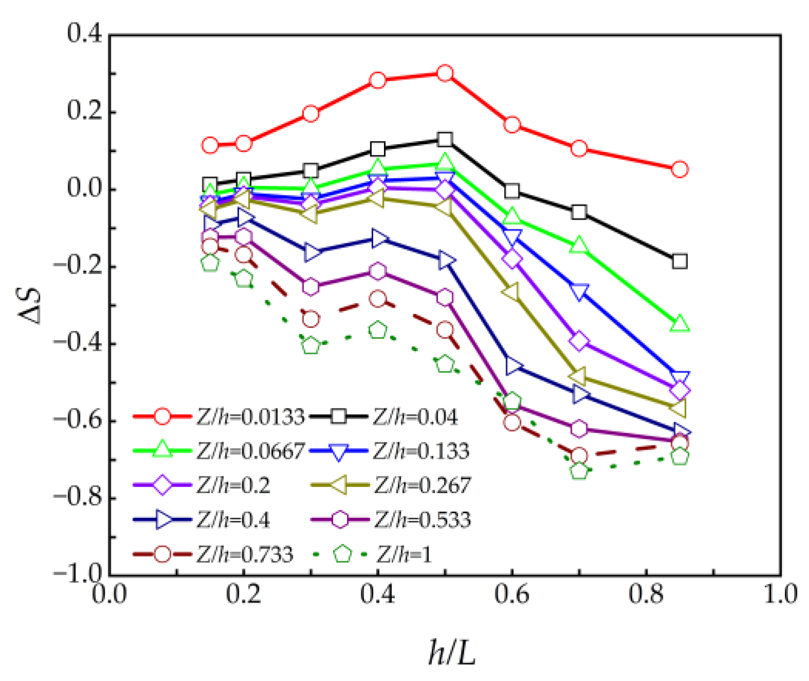
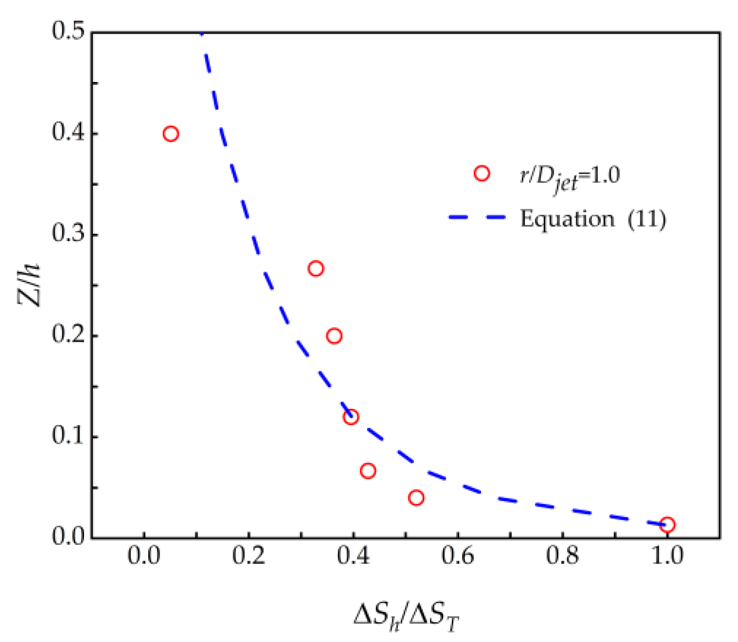
3.3. Modeling Based on the Height of the Hill above the Ground

The above two subsections have obtained the speedup ratio equations for leeward, windward, and near-ground of the hilltop considering the slope and radial distance. Next, analyze the variation of hilltop speedup ratio with height above ground at different radial distances.
Combining Equation (9) with Equation (10) yields the speedup ratio at the hilltop for any radial position and hill slope, whereby the speedup ratio at any position along the hill surface can be obtained according to Equations (7) and (8). To establish a comprehensive wind field model for downburst flow over hilly terrain, the distribution of the speedup ratio along the vertical height of the hill is considered. In Figure 5 and Figure 10, the speedup ratios on the windward and leeward foothills display a deceleration effect. In contrast, the speedup effect increases with the vertical height, but the horizontal wind speed is smaller at higher heights. In contrast, a larger speedup ratio appears at the hilltop, so the speedup ratios at the hilltop at different radial positions are selected for analysis. As shown in Figure 14, the speedup ratio is smaller and decays faster with height for the radial position greater than 1.5 Djet. The deceleration effect appears at the hilltop when the vertical height is below 0.1h. Therefore, only the variation of the hilltop speedup ratio with vertical height for the radial position less than 1.5 Djet position is considered.
As shown in Figure 14, the speedup ratio at the hilltop can be obtained from Equation (9), so the speedup ratio at the hilltop is dimensionless and used to investigate the variation of the speedup ratio with vertical height. At a vertical height of 0.45h and a radial position of 1.0 Djet, the hill’s speedup ratio displays a deceleration effect, and this trend remains consistent until then. In order to ensure the effectiveness and universal applicability of the model, a working condition was selected where the speedup ratio changes gradually with vertical height. Specifically, the speedup ratio of a hill at a radial position of 1.0 Djet was selected as the basis for model development.
The expressions for the variation of the speedup ratio of the hill with height are shown below, as shown in Figure 15. That is, when the vertical height is below 0.2h, the predicted speedup ratio values of the model are all greater than those of numerical simulation. However, a deceleration effect occurs when the hill height exceeds 0.5h, which means the speedup effect is not considered at this point.
Δ S h Δ S T = ( Z h ) 0.161 1.01
where Z 0.5 h , and ΔSh is the hilltop speedup ratio at different heights.
Figure 16 shows the dimensionless speedup ratios at the hilltop of different slopes located at the radial position of 1.5 Djet. The speedup ratios are dimensionless based on that at the hilltop and compared with Equation (11). It is found that the speedup ratios of each hill slope decayed more slowly than Equation (11) after dimensionless with the speedup ratios at the hilltop; so, it can be considered that Equation (11) can be used to describe the variation of the speedup ratios of the hill with vertical height. The prediction results are larger and relatively conservative than the numerical simulation values. According to Figure 7, it can be seen that the range of speedup ratio in the hilly area is mostly concentrated in the range zh/h > 0.5, so only in this range the speedup effect is considered, and the rest of the locations are deceleration effects. The speedup effect is not considered in the design of the building structure, and the wind speed of flat terrain is used for structural design.

3.4. Verification of the Semiempirical Model

In the previous section, the variation of the speedup ratio with the hill slope, radial distance, and vertical height for the hill at the hilltop and at the foothill on the leeward side is studied; based on this, the semiempirical model of the speedup ratio of the downburst winds distribution along the hill model is established, and the above results are verified in this section.
The radial positions of 1.3 Djet and 1.7 Djet are to ensure the accuracy of the model, considering the speedup ratios of the hill placed at different radial positions. The hilltop speedup ratios at the 1.3 Djet and 1.5 Djet positions are calculated according to Equation (9). Then the hilltop speedup ratios at the windward side can be obtained according to Equation (7). Then the distributed speedup ratios at the leeward side can be obtained according to Equation (8). Table 3 gives the distribution of speedup ratios at different radial positions at the hilltop and foothill on the leeward side. It can be seen from Table 3 that the predicted hilltop speedup ratios at the 1.7 Djet and 1.3 Djet positions are close to the simulated values, and the predicted maximum values at 1.3 Djet are closer to the simulated values. The predicted maximum speedup values at 1.7 Djet are smaller than the simulated values, with some differences.
Figure 17 shows the distribution of speedup ratios at 1.3 Djet and 1.7 Djet radial positions along the hill model. From Figure 17a, it can be learned that the measured and tested values match better when the speedup ratio values are near the hilltop, the simulation accuracy of 1.3 Djet is higher than the results of 1.7 Djet, and the predicted values of 1.7 Djet are overall smaller than the simulated values. As shown in Figure 17b, the speedup ratios at each radial position show a linear relationship with the change in downstream distance, and the predicted values at both positions agree with the simulated values. Overall, it is believed that the accuracy of using the model which changes with the radial position of the hill to calculate the distribution of speedup ratios is high.
The hill models with a slope of 0.35 and 0.65 at the foot of the hill are selected to compare speedup ratios. The speedup ratios obtained at each location are shown in Table 4, and the speedup ratios distributed along the hill model are shown in Figure 16.
When using the hill model, the speedup ratio of the hill at the hilltop position is firstly derived from Equation (10) based on the existing slope, the speedup ratio of the windward foot at each position is derived from Equation (7), and then the speedup ratio of the leeward position is solved from Equation (8). The results are shown in Table 4. The maximum speedup ratios obtained by the model are closer to those obtained from numerical simulations when the slope is 0.35. At a slope of 0.65, the speedup ratio obtained by this model at the hilltop position is greater than the numerical simulation value, and there is also some difference in the maximum value.
Figure 18a illustrates that the predicted speedup ratios of the hill on the windward side, as proposed in this paper, match well with the numerical simulation results when the slope angle is 0.35. However, the predicted results are lower than the simulated values in the hilltop region when the slope angle is 0.65. Nevertheless, the decay of the numerical simulation results is comparatively slower than the predicted values near the foot of the windward side. In Figure 18b, when the speedup ratios at the hilltop location and the foot of the leeward side are analyzed in a linear relationship, the outcomes demonstrate wide variation and do not show a linear decrease. Particularly, when the slope is small, the predicted results are lower than the simulated values, but when the slope is large, the predicted results are the opposite and greater than the simulated values. Hence, there is still a need for further improvement in the model when considering the deceleration effect on the leeward side.
Figure 19 confirms the change in the speedup ratio concerning the height direction at the hilltop point for various locations. The outcomes for the speedup ratios agree with the model’s predictions at the near-ground location. However, at the radial position of 1.3 Djet, the predicted speedup ratios are lower than the numerical simulation results. Moreover, the values of speedup ratios acquired from Equation (11) decrease comparatively slower and are higher than the numerical simulation results, indicating a relatively conservative prediction.

4. Conclusions

This paper primarily conducts numerical simulations to investigate the development of a speedup ratio model for downbursts over hilly terrains. The experimental results are compared with those of several turbulence models to determine the most accurate and computationally efficient one. The chosen turbulence model is then employed to examine the impact of hill parameters on the speedup ratio, and the parameter variations are used to construct a distribution of the speedup ratio close to the ground. As a result, the main conclusions drawn from this study can be summarized as follows.
  • By comparing the numerical simulation results for the wind field over the hill from three turbulence models with the average experimental wind speed, it was found that the accuracy of the REA k-ε model in the RANS model was higher than that of the other models.
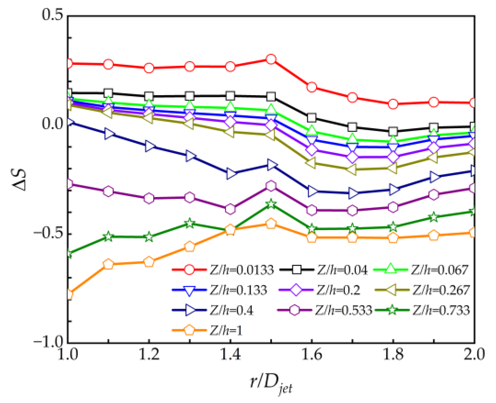
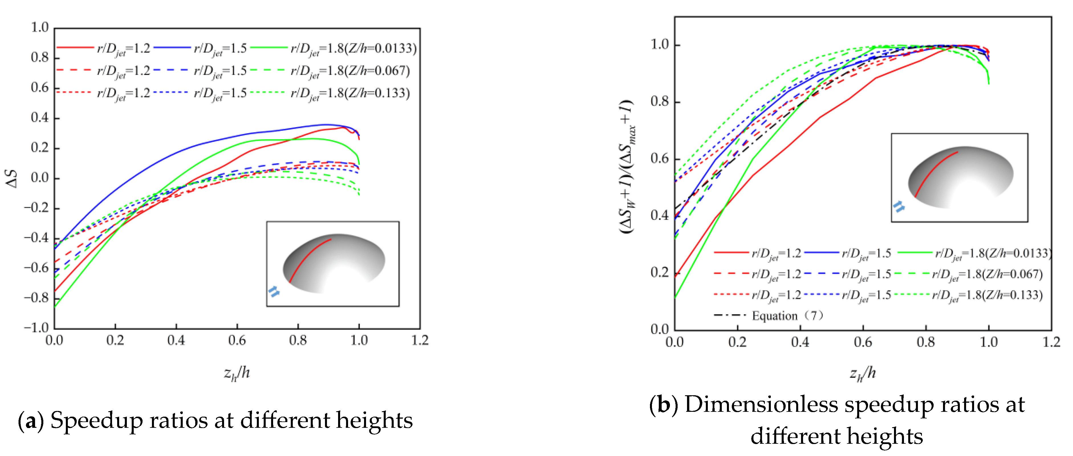
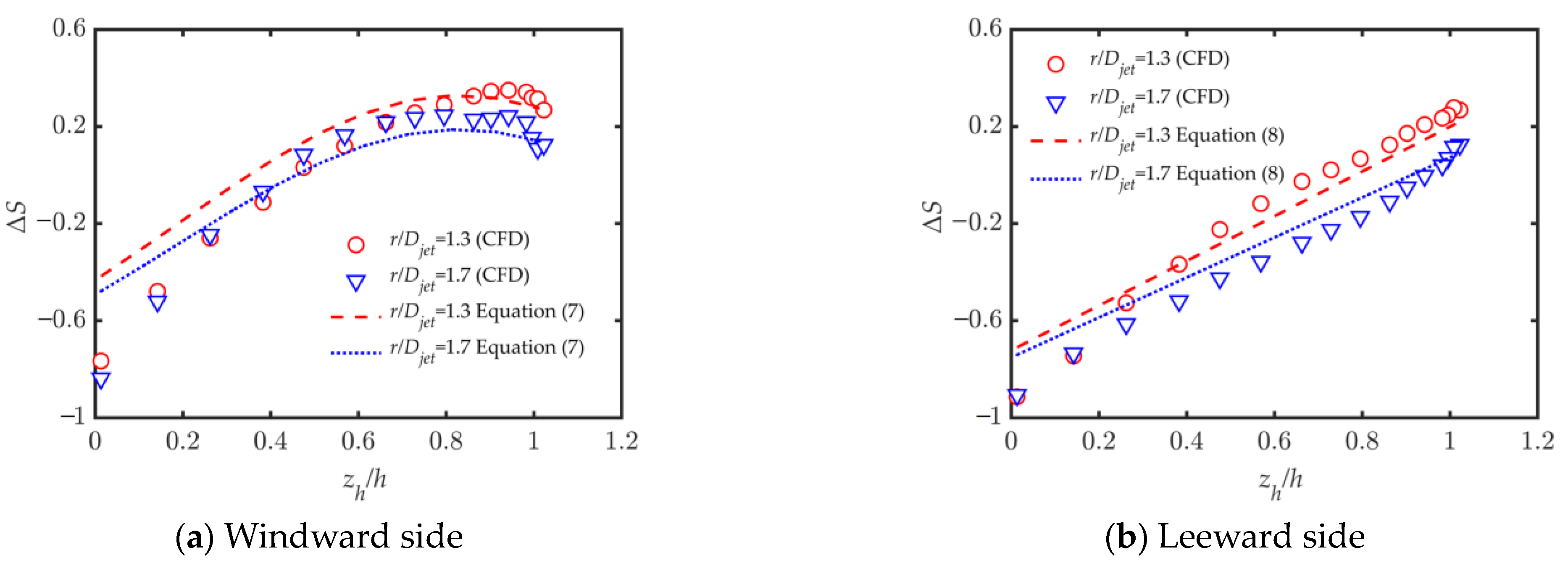
  • When using the same hill model at various radial locations, the maximum speedup ratio is observed at the windward side, typically occurring between 0.7h to 0.9h. The distribution of speedup ratios at each radial location has the same trend. The values of speedup ratios distributed along the hill model at each radial location can be obtained when the hilltop speedup ratio at each location can be predicted. The speedup ratio model of hilly terrain was validated for different radial distances, and the results showed that the model has high accuracy.
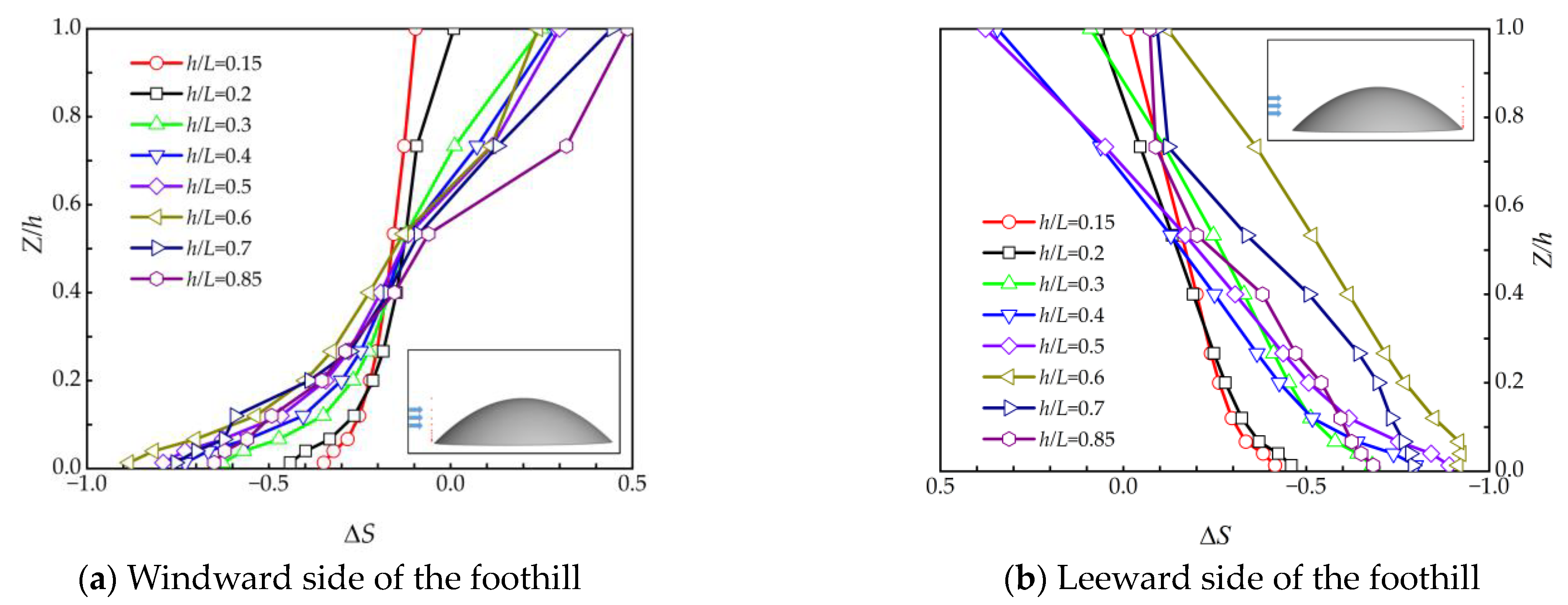
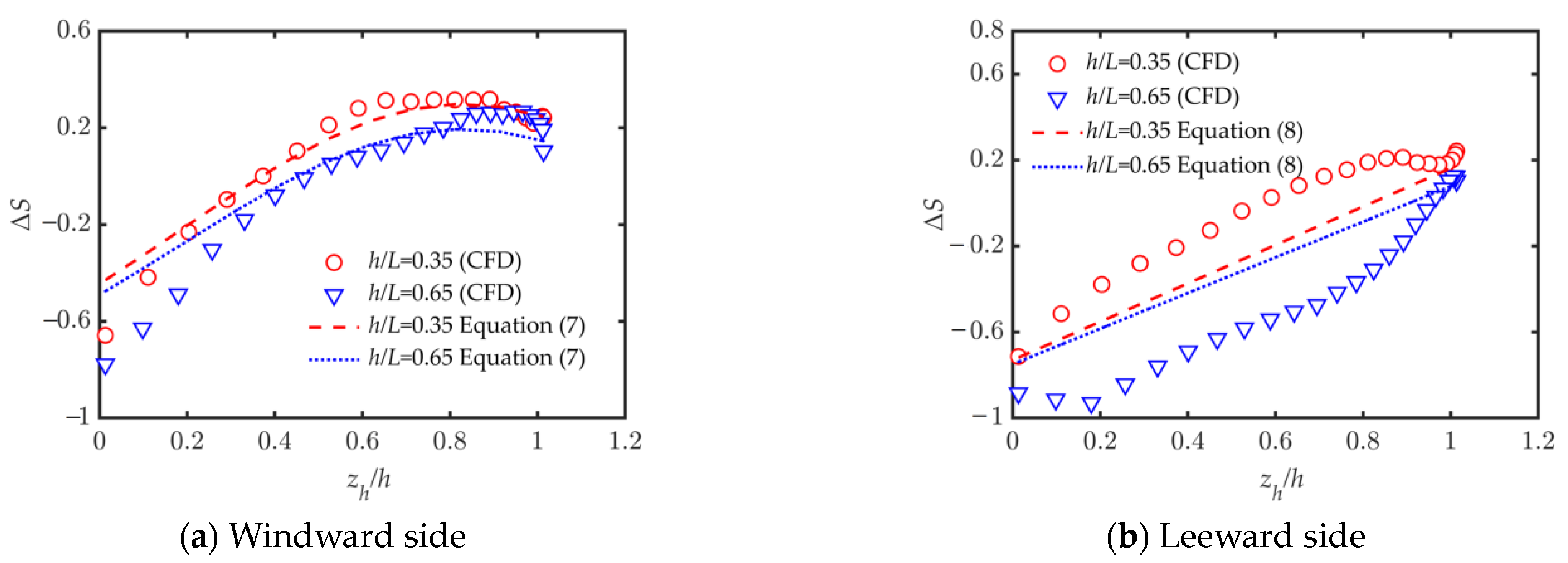
  • By changing different slopes, the model of speedup ratio distributed along the hill model was constructed. The trend of the speedup ratio distribution on the windward side was consistent, while on the leeward side it showed a linear decay. The model’s accuracy was confirmed through further validation, demonstrating its capability for predicting the speedup ratio on the windward side of the hill. Numerical simulations showed good agreement with the model, and the conservative prediction of the speedup ratio near the hilltop was confirmed. However, further improvement is necessary to consider the deceleration effect on the leeward side of the hill.
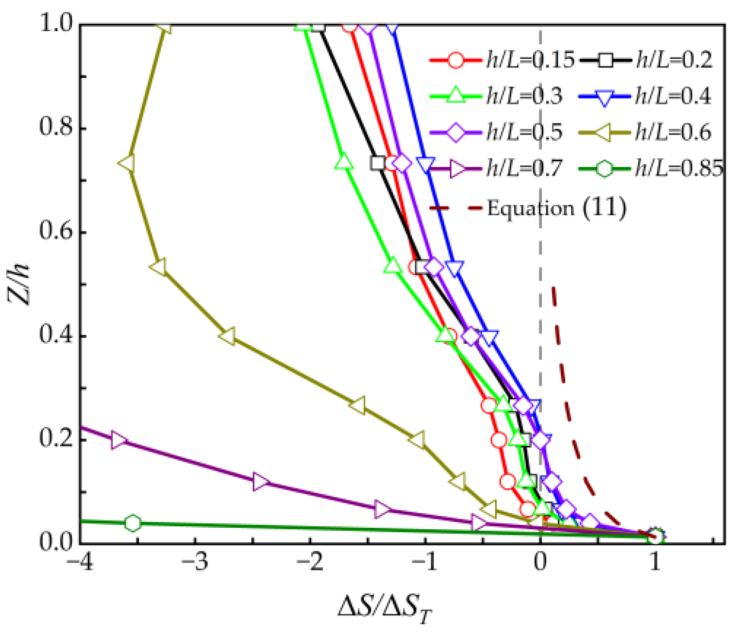
  • The speedup ratio near the ground at the hilltop can be obtained from the above study. To establish a complete model, the distribution of the speedup ratio along the height of the hill is considered. Through this study, it was found that the speedup effect typically occurs at heights of 0.5h or greater. As a result, the model focuses on this range for predicting speedup ratios. Further validation along the height direction confirms the model’s accuracy in predicting speedup ratios at locations near the ground.
While the main focus of this paper is the construction of a semiempirical model for downburst speedup ratios over hills, the potential for further research is significant. First, more complex terrain such as double ridges, steep slopes, and actual terrain can be explored to expand the model’s applicability. Additionally, the empirical model can be improved by utilizing a combination of measured data and mesoscale simulations to obtain more realistic meteorological information.

Author Contributions

Funding acquisition, B.Y.; Methodology, C.M.; Project administration, B.Y.; Validation, Y.H.; Writing—original draft, B.Y., Y.H.; Writing—review & editing, X.C. All authors have read and agreed to the published version of the manuscript.

Funding

This research was funded by the National Natural Science Foundation of China (No. 51720105005 and No. 51878104), the 111 Project (B18062), the Natural Science Foundation of Chong-qing, China (cstc2022ycjh-bgzxm0050) and Fundamental Research Funds for the Central Universi-ties (2022CDJQY-009).

Data Availability Statement

No new data were created or analyzed in this study. Data sharing is not applicable to this article.

Conflicts of Interest

The authors declare no conflict of interest.

References

  1. Fujita, T.T. Tornadoes and downbursts in the context of generalized planetary scales. J. Atmos. Sci. 1981, 38, 1511–1534. [Google Scholar] [CrossRef]
  2. Elawady, A.; Aboshosha, H.; El Damatty, A.; Bitsuamlak, G.; Hangan, H.; Elatar, A. Aero-elastic testing of multi-spanned transmission line subjected to downbursts. J. Wind Eng. Ind. Aerodyn. 2017, 169, 194–216. [Google Scholar] [CrossRef]
  3. Holmes, J.D.; Hangan, H.M.; Schroeder, J.L.; Letchford, C.W.; Orwig, K.D. A forensic study of the Lubbock-Reese downdraft of 2002. Wind Struct. 2008, 11, 137–152. [Google Scholar] [CrossRef]
  4. Solari, G.; De Gaetano, P.; Repetto, M.P. Thunderstorm response spectrum: Fundamentals and case study. J. Wind Eng. Ind. Aerodyn. 2015, 143, 62–77. [Google Scholar] [CrossRef]
  5. Ministry of Housing and Urban-Rural Development of the People’s Republic of China. Load Code for the Design of Building Structures; China Architecture & Building Press: Beijing, China, 2012. [Google Scholar]
  6. Homar, V.; Gaya, M.; Romero, R.; Ramis, C.; Alonso, S. Tornadoes over complex terrain: An analysis of the 28th August 1999 tornadic event in eastern Spain. Atmos. Res. 2003, 67, 301–317. [Google Scholar] [CrossRef] [Green Version]
  7. Wang, Q.; Luo, K.; Wu, C.; Mu, Y.; Tan, J.; Fan, J. Diurnal impact of atmospheric stability on inter-farm wake and power generation efficiency at neighboring onshore wind farms in complex terrain. Energy Convers. Manag. 2022, 267, 115897. [Google Scholar] [CrossRef]
  8. Wang, Q.; Luo, K.; Wu, C.; Zhu, Z.; Fan, J. Mesoscale simulations of a real onshore wind power base in complex terrain: Wind farm wake behavior and power production. Energy 2022, 241, 122873. [Google Scholar] [CrossRef]
  9. Wang, Q.; Luo, K.; Yuan, R.; Zhang, S.; Fan, J. Wake and performance interference between adjacent wind farms: Case study of Xinjiang in China by means of mesoscale simulations. Energy 2019, 166, 1168–1180. [Google Scholar] [CrossRef]
  10. Selvam, R.P.; Holmes, J.D. Numerical simulation of thunderstorm downdrafts. J. Wind Eng. Ind. Aerodyn. 1992, 44, 2817–2825. [Google Scholar] [CrossRef]
  11. Letchford, C.W.; Illidge, G.C. Turbulence and Topographic Effects in Simulated Thunderstorm Downdrafts by Wind Tunnel Jet; Wind Engineering into the 21th Century: Copenhagan, Denmark, 1999; pp. 1907–1912. [Google Scholar]
  12. Mason, M.S.; Wood, G.S.; Fletcher, D.F. Impinging jet simulation of stationary downburst flow over topography. Wind Struct. 2007, 10, 437–462. [Google Scholar] [CrossRef]
  13. Abd-Elaal, E.S.; Mills, J.E.; Ma, X. Numerical simulation of downburst wind flow over real topography. J. Wind Eng. Ind. Aerodyn. 2018, 172, 85–95. [Google Scholar] [CrossRef]
  14. Huang, G.Q.; Jiang, Y.; Peng, L.L.; Solari, G.; Liao, H.L.; Li, M.S. Characteristics of intense winds in mountain area based on field measurement: Focusing on thunderstorm winds. J. Wind Eng. Ind. Aerodyn. 2019, 190, 166–182. [Google Scholar] [CrossRef]
  15. Burlando, M.; Romanić, D.; Solari, G.; Hangan, H.; Zhang, S. Field data analysis and weather scenario of a downburst event in Livorno, Italy, on 1 October 2012. Mon. Weather Rev. 2017, 145, 3507–3527. [Google Scholar] [CrossRef]
  16. Canepa, F.; Burlando, M.; Solari, G. Vertical profile characteristics of thunderstorm outflows. J. Wind Eng. Ind. Aerodyn. 2020, 206, 104332. [Google Scholar] [CrossRef]
  17. Jackson, P.S.; Hunt, J. Turbulent wind flow over a low hill. Q. J. R. Meteorol. Soc. 1975, 101, 929–955. [Google Scholar] [CrossRef]
  18. Taylor, P.A. Turbulent boundary-layer flow over low and moderate slope hills. J. Wind Eng. Ind. Aerodyn. 1998, 74, 25–47. [Google Scholar] [CrossRef]
  19. Weng, W.; Taylor, P.A.; Walmsley, J.L. Guidelines for airflow over complex terrain: Model developments. J. Wind Eng. Ind. Aerodyn. 2000, 86, 169–186. [Google Scholar] [CrossRef]
  20. Oseguera, R.M.; Bowles, R.L. A Simple, Analytical 3-Dimentional Downburst Model Based on Boundary Layer Stagnation Flow; No. NASA-TM-100632; NASA: Hampton, VA, USA, 1988. [Google Scholar]
  21. Vicroy, D.D. Assessment of microburst models for downdraft estimation. J. Aircr. 1992, 29, 1781–1787. [Google Scholar] [CrossRef]
  22. Holmes, J.D.; Oliver, S.E. An empirical model of a downburst. Eng. Struct. 2000, 22, 1167–1172. [Google Scholar] [CrossRef]
  23. Li, C.; Li, Q.S.; Xiao, Y.Q.; Ou, J.P. A revised empirical model and CFD simulations for 3D axisymmetric steady-state flows of downbursts and impinging jets. J. Wind. Eng. Ind. Aerodyn. 2012, 102, 48–60. [Google Scholar] [CrossRef]
  24. Hjelmfelt, M.R. Structure and Life Cycle of Microburst Outflows Observed in Colorado. J. Appl. Meteorol. 1988, 27, 900–927. [Google Scholar] [CrossRef]
  25. Boussinesq, J. Essai sur la théorie des eaux courantes; Imprimerie Nationale: Paris, France, 1877. [Google Scholar]
  26. Yakhot, V.; Orszag, S.A. Renormalization group analysis of turbulence. I. Basic theory. J. Sci. Comput. 1986, 1, 3–51. [Google Scholar] [CrossRef]
  27. Tsan-Hsing, S.; William, W.L.; Aamir, S. A new k-ε eddy viscosity model for high Reynolds number turbulent flows: Model development and validation. Comput. Fluids 1995, 24, 30. [Google Scholar]
  28. Menter, F.R. Two-equation eddy-viscosity turbulence models for engineering applications. AIAA J. 1994, 32, 1598–1605. [Google Scholar] [CrossRef] [Green Version]
  29. Kari, E.; Kratzer, S.; Beltrán-Abaunza, J.M.; Harvey, E.T.; Vaičiūtė, D. Retrieval of suspended particulate matter from turbidity–model development, validation, and application to MERIS data over the Baltic Sea. Int. J. Remote Sens. 2017, 38, 1983–2003. [Google Scholar] [CrossRef] [Green Version]
Figure 1. Flowchart illustrating the methodology for numerical simulations.
Atmosphere 14 00694 g001
Figure 2. Computational domain, boundary conditions, and grid arrangements.
Atmosphere 14 00694 g002
Figure 3. Illustration of the wind tunnel test.
Atmosphere 14 00694 g003
Figure 4. Comparison of mean velocity between different turbulence models and experiments.
Atmosphere 14 00694 g004
Figure 5. Speedup ratio of the hill with different radial positions.
Atmosphere 14 00694 g005
Figure 6. Hilltop speedup ratio at different radial positions.
Atmosphere 14 00694 g006
Figure 7. Speedup ratio along the windward side of the hill model.
Atmosphere 14 00694 g007
Figure 8. Speedup ratio along the leeward side of the hill model.
Atmosphere 14 00694 g008
Figure 9. Change of speedup ratio with radial position (Z/h = 0.0133).
Atmosphere 14 00694 g009
Figure 10. Speedup ratio of the hill with different slopes.
Atmosphere 14 00694 g010aAtmosphere 14 00694 g010b
Figure 11. Hilltop speedup ratio with different slopes.
Atmosphere 14 00694 g011
Figure 12. Speedup ratio of different slopes (Z/h = 0.0133).
Atmosphere 14 00694 g012
Figure 13. The change in speedup ratio at the hilltop with the slope of the hill (Z/h = 0.0133).
Atmosphere 14 00694 g013
Figure 14. The dimensionless speedup ratio at the vertical height of the hilltop.
Atmosphere 14 00694 g014
Figure 15. Variation of speedup ratio with vertical height.
Atmosphere 14 00694 g015
Figure 16. Dimensionless speedup ratio at vertical height.
Atmosphere 14 00694 g016
Figure 17. Validation of hill Speedup ratio model for different radial positions.
Atmosphere 14 00694 g017
Figure 18. Validation of hill speedup ratio model for different slopes.
Atmosphere 14 00694 g018
Figure 19. Validation of Speedup ratio for vertical distribution at the hilltop.
Atmosphere 14 00694 g019
Table 1. Analysis of velocity error between different turbulence models and experiments.
ErrorRealizable k-εSST k-ωRNG k-ε
10%57.14%38.57%40%
20%75.71%54.29%70%
30%85.71%71.43%81.43%
MNB2.04%2.95%5.94%
Table 2. Parameter settings for hill models.
Model Numberh (mm)L (mm) ϕ (Slope)
Quad-L500-H075755000.15 (8.53°)
Quad-L375-H075753750.2 (11.3°)
Quad-L225-H075752250.3 (16.7°)
Quad-L187-H07575187.50.4 (26.6°)
Quad-L150-H075751500.5 (8.53°)
Quad-L125-H075751250.6 (31°)
Quad-L107-H07575107.50.7 (35°)
Quad-L088-H07575880.85 (40.36°)
Table 3. Speedup ratio of different radial positions.
1.3 Djet1.7 Djet
HilltopMaximumHilltopMaximum
CFD0.26840.34980.12590.2433
Model Prediction0.26250.33130.12900.1905
Table 4. Speedup ratio of different slopes.
0.350.65
HilltopMaximumHilltopMaximum
CFD0.24270.31840.10360.2628
Model Prediction0.22320.30150.13530.1972
Disclaimer/Publisher’s Note: The statements, opinions and data contained in all publications are solely those of the individual author(s) and contributor(s) and not of MDPI and/or the editor(s). MDPI and/or the editor(s) disclaim responsibility for any injury to people or property resulting from any ideas, methods, instructions or products referred to in the content.

