1. Introduction
The ionosphere is regarded as the part of the atmosphere with the maximum concentration of ions and electrons that lies between 80 km and 300 km altitudes. It is then defined as the region in the Earth’s atmosphere with the largest number of free electrons and ions that have the ability to affect radio waves. The ionosphere is highly variable in space and time (sunspot cycle, seasonal, and diurnal periods), also depending on geographical location (polar, aurora zones, mid-latitudes, and equatorial regions) and on certain solar-related ionospheric disturbances. Ionosphere research has attracted significant attention from the Global Positioning System (GPS) community because the ionosphere’s range delay on GPS signals is a major error source in GPS positioning and navigation. The ionosphere has practical importance in GPS applications because it influences trans-ionospheric radio wave propagation. The ionosphere causes GPS signal delays to be proportional to the total electron content (TEC) along the path from the GPS satellite to a receiver. The TEC is defined by the integral of electron density in a 1 m squared column along the signal transmission path. The TEC is a key parameter in the mitigation of ionospheric effects on the radio system. The TEC measurements obtained from dual-frequency GPS receivers are one of the most important methods for investigating the Earth’s ionosphere [
1].
In addition, with the random fluctuations in the amplitude and phase of trans-ionospheric radio signals, ionospheric plasma irregularities have become a continuous and major concern for satellite communication systems. Previous studies have shown that ionospheric scintillations are most likely to occur near the magnetic equator in the post-sunset period [
2,
3,
4,
5,
6]. These irregularities are caused by plasma instability typically formed at the bottom of the F-region during the post-sunset period due to the Rayleigh–Taylor (R-T) instability mechanism. Post-sunset, the absence of solar radiation causes the lower ionosphere to rapidly decay, thereby increasing the bottom side of the F-layer. This is synonymous with a heavy fluid being situated above a light fluid [
7]. Such a contrast in density leads to the mixing of the two layers by forming bubbles and spikes. As the bubbles develop, there is a rapid local variation in the refractive index of the Earth’s ionosphere through which radio signals traverse. The effect of these density abnormalities manifests as signal amplitude and/or phase fluctuations called ionospheric scintillation [
3]. These fluctuations cause significant degradation of trans-ionospheric signals, resulting in signal fading below the fade margin of the receiver, and could lead to signal loss and cycle slips [
4,
8]. However, these effects have been investigated using GPS receivers for many years [
4,
5,
9,
10,
11]. For instance, [
2] investigated the irregularities in Lagos state, Nigeria, using GPS observations during the 2009–2011 period. They reported that the equinoctial months recorded the highest occurrence of irregularities, while the lowest was recorded during the June solstices. In addition, [
12] studied the trend of the ionospheric irregularities in Africa using ROTI derived from Global Navigation Satellite System (GNSS) data. They found that irregularities occurred from March to November, with a minimum observed around June and very low activity around January. Despite the various studies conducted in Africa, particularly in the equatorial region where Nigeria is located, no GPS receivers have been operational in Nigeria since the year 2018. As a result of this, the characteristics of the varying ionosphere over Nigeria are not known. This led to the installation of a Connected Autonomous Space Environment Sensor (CASES) GPS receiver at Bowen University in Iwo, Osun State, Nigeria. The Center for Space Science and Engineering Research (Space@VT) at Virginia Polytechnic Institute and State University, Blacksburg, Virginia, in the United States and Bowen University, Nigeria, collaborated on the deployment of a CASES GPS receiver.
The CASES GPS receiver differs from standard GNSS receivers in two important ways: it was specifically made to measure TEC and scintillation parameters, and it has a unique feature that enables it to function reliably in the presence of strong ionospheric scintillation. Since there are no GPS receivers around that record scintillation measurements, measurements of the TEC and ionospheric irregularities from this newly installed CASES GPS receiver will be investigated. A comparison of the CASES GPS receiver will be made with a typical GNSS receiver located in a nearby country, the Benin Republic (BJCO).
Section II of this introduction includes a description of the CASES’s hardware platform and the performance specifications.
Section 2 is about the data and methodology we employed in this investigation. We present all our important results and discussions in
Section 3.
Section 4 is about our conclusions.
2. The CASES Hardware Platform
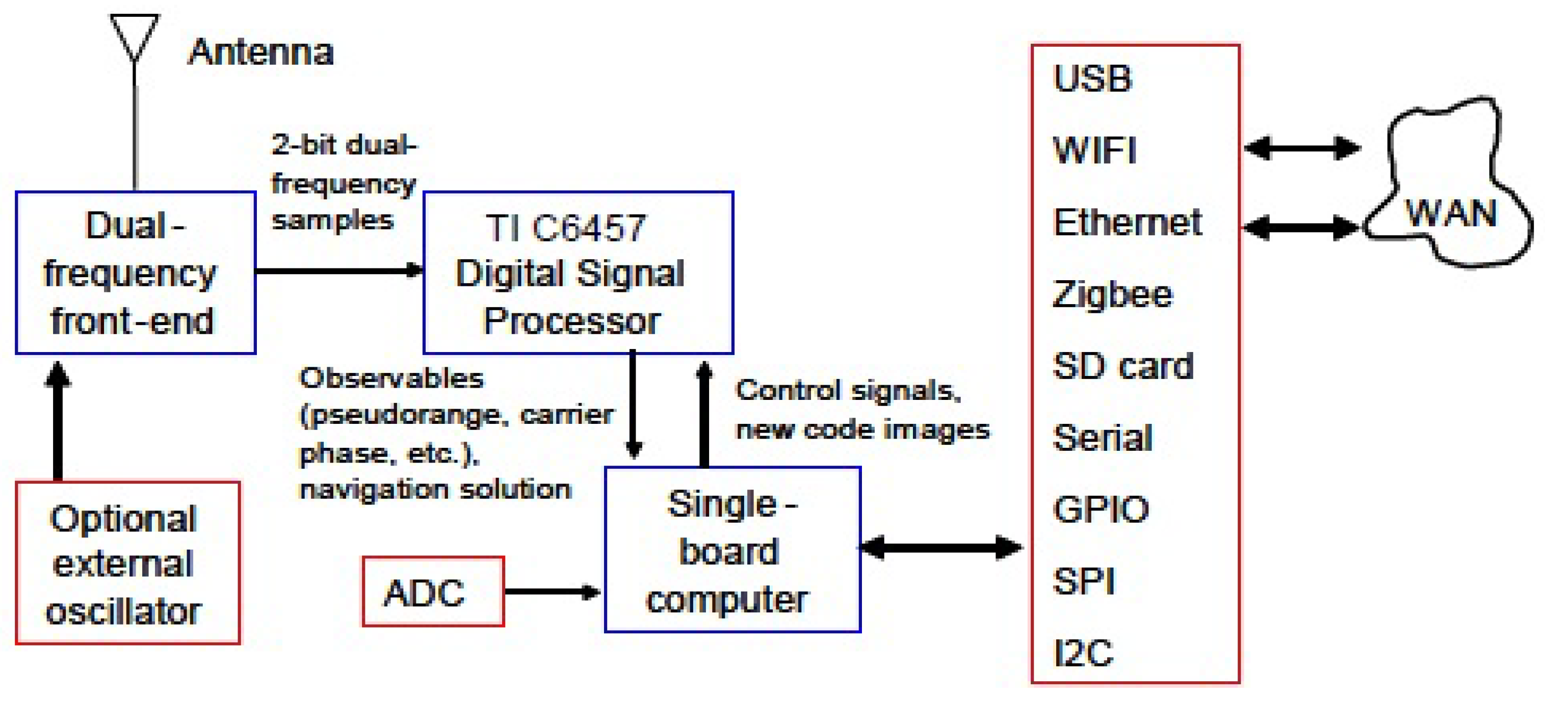
The CASES GPS receiver was made with the intention of offering a powerful platform with a wide range of peripheral options, as it is inexpensive, compact, and power-efficient. The final configuration consists of three parts, namely: a custom-built dual frequency, a digital signal processor board, and a “single board computer” with an ARM microcontroller.
Figure 1 depicts a block schematic of the receiver hardware, and
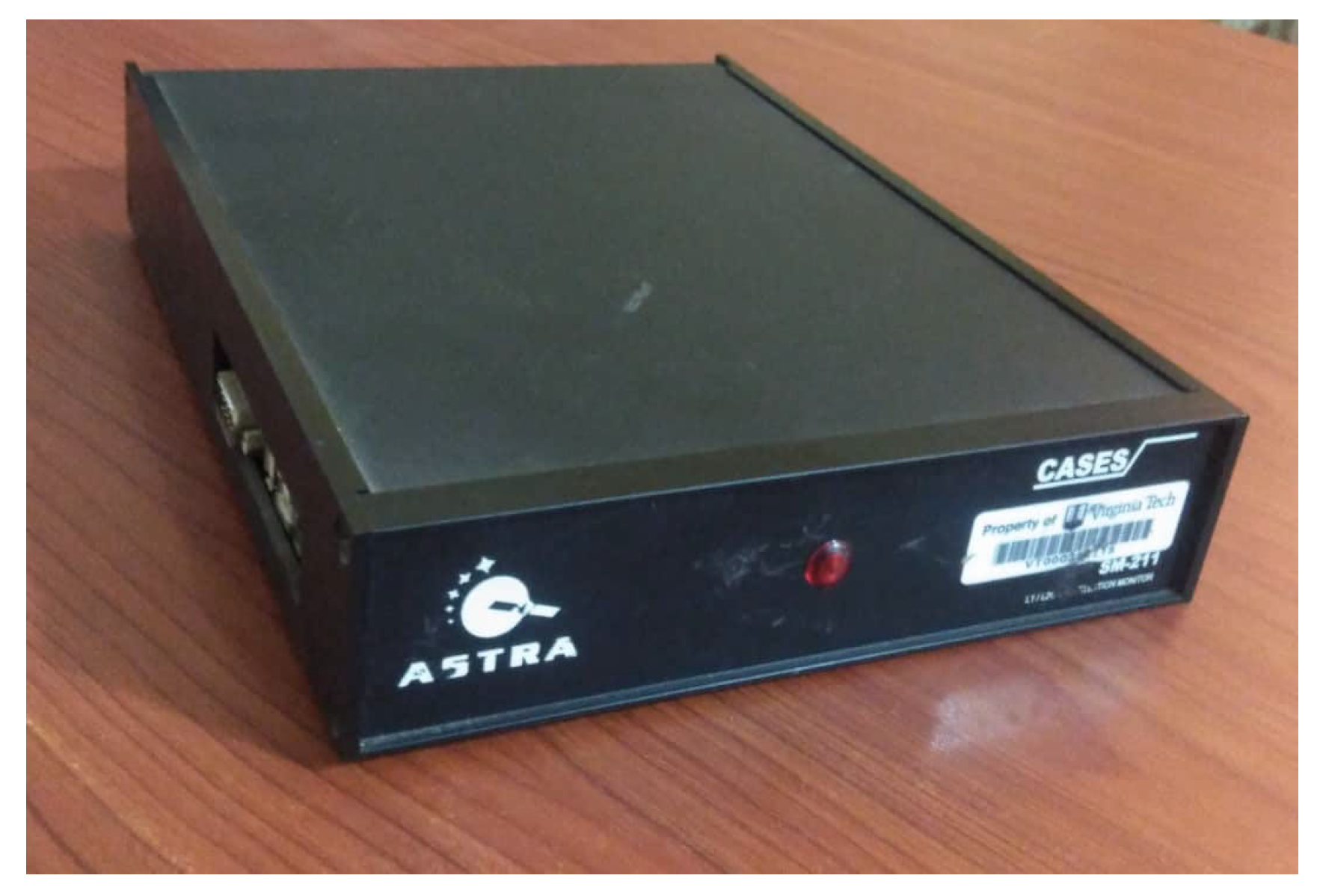
Figure 2 shows a photo of a CASES GPS receiver and antenna.
The dual-frequency back end generates 2-bit samples at a rate of 5.7 samples/second within a constrained bandwidth of 2.4 MHz that produces one set of 2-bit samples for each of the L1 and L2 GPS frequencies. In addition, the automatic gain-controlled amplification, filtering, mixing to an intermediate frequency, and sampling are all performed by this front end.
The back end provides an optional input for attaching an external 10 MHz frequency reference, with the termination of 50 or 1000 Ohms, and can supply a chosen 5-volt DC bias on the antenna input to power active antennas. The board uses about 360 milliamps at 5 volts, excluding any power needed by an active antenna that is connected. Despite the non-negligible changes in the measured carrier phase that a temperature-compensated crystal oscillator (TCXO) introduces [
13], both frequencies are sampled concurrently, with the frequency reference provided by an onboard TCXO.
A general-purpose digital signal processor handles all processing for the CASES GPS receiver, a software-defined receiver. A Texas Instruments C6457 digital signal processor is housed on a second custom-built board (DSP). The processor contains 4MB of non-volatile flash memory, 128 MB of off-chip RAM, and a 1 GHz clock speed. It also has 2 MB of on-chip RAM. All acquisition and tracking tasks, as well as the computation of the navigation solution and different observables including pseudo-range, beat carrier phase, and Doppler shift, is carried out by the DSP board. The board outputs the beat carrier phase, timestamps, in-phase and quadrature accumulations, and other data at 10 Hz or less. Approximately 75% of the processor is used when tracking 12 GPS L1 C/A code channels and 4 GPS L2CL channels, computing the navigation solution, acquiring continuous background signals, and carrying out all additional overhead. At 5 volts, the DSP board uses about 580 milliamps.
A “single-board computer” (SBC) running the GNU/Linux operating system makes up the third main reception component. An ARM AT91SAM9260 microcontroller with a wide range of available peripherals powers the SBC. This board has 128 MB of flash memory for the file system and 32 MB of RAM. Ethernet, a serial peripheral interface, a secure digital card reader, a universal serial bus, ZigBee, Wi-Fi, a 10-bit analog-to-digital converter, and general-purpose I/O pins are among the peripherals that are offered. Images or configuration files are frequently used for communication, along with an RS232 serial port, Ethernet, or Wi-Fi. The SBC also maintains a secure shell server that enables remote log-in for additional tasks that the server application does not provide. At 5 volts, the SBC uses about 260 milliamps. The SBC is equipped with a network-connected server application that enables remote data logging, code image or configuration file upload, and monitoring. It also maintains a secure shell server that enables remote log-in for additional tasks that the server application does not provide. At 5 volts, the SBC uses about 260 milliamps. Detailed descriptions of the CASES GPS receiver can also be found in the works of [
14,
15].
This Connected Autonomous Space Environment Sensor (CASES) from ASTRA is a software-defined GPS receiver with the dual frequency of L1 C/A and L2C codes for space-weather monitoring and can be remotely programmed via an internet source. The receiver employed numerous novel techniques that make it suitable for space-weather studies compared to other nearby GPS such as the different methods for eliminating local clock effects, advanced triggering mechanism for determining scintillation onset, data buffering to permit observation of the prelude to scintillation, and data-bit prediction and wipe-off for robust tracking. More so, the CASES hardware is made up of a custom-built dual frequency, a digital signal processor board, and a “single board computer” with an ARM microcontroller.
3. Methodology
Data received from GPS satellites have been very useful in TEC estimation across the Earth. In an effort to understand ionospheric irregularities at the equatorial region, a new Connected Autonomous Space Environment Sensor (CASES) GPS scintillation monitoring receiver was installed at Bowen University, Iwo, Osun State, Nigeria, in June 2019. This is in collaboration with the Center for Space Science and Engineering Research (Space@VT) at Virginia Polytechnic Institute and State University, Blacksburg, VA, USA. The objective of the collaboration involves a detailed investigation of the characteristics of Nigeria’s equatorial ionosphere. With these initiatives, more GPS receivers have been made available for space weather observations in lieu of the very expensive commercial brands.
The CASES GPS receiver is set to operate at L1 (1575.42 MHz) and L2 (1227.60 MHz) band frequencies. It can measure the ionospheric irregularities or electron density fluctuations in the ionosphere with varying sampling rate schemes every three minutes.
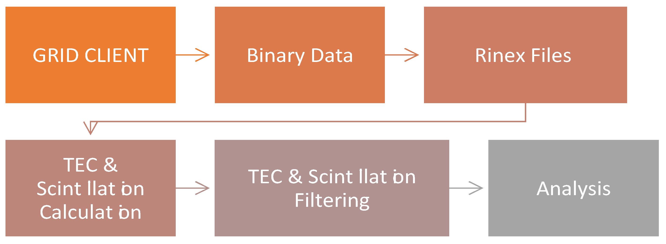
Figure 3 shows the data processing chain using the CASES GPS receiver. The Grid client software enables the data that are in binary digits to be logged into the local machine. For data post-processing, the method described by [
16] is used to remove the receiver clock effects and eliminate low-frequency effects, including tropospheric effects, satellite motion, and the multipath passed through a high pass filter. To eliminate the effect of multipath, a minimum elevation angle of 20° was used. The VTEC data estimated are then subjected to a two-sigma (2 s) iteration, which is a measure of GPS point positioning accuracy (95% confidence level). This 95% confidence level corresponds to 1.96 standard deviations, which is then approximate to two standard deviations or 2 s, and the resulting values are the average of VTEC over all pseudorandom numbers (PRNs) on a day.
Therefore, the data used for this investigation were collected from the newly installed Connected Autonomous Space Environment Sensor (CASES) GPS receiver for the period of January–December 2021 with the following coordinates: Latitude: 7.62° N, Longitude: 4.14° E, Diplat: 2.36° S. In addition, the GPS-TEC data for station BJCO in Cotonou, Benin Republic (Latitude: 6.38° N, Longitude: 2.45° E, Diplat: 3.08° S) were also retrieved for the period of January–December 2010 from
https://www.sonel.org/ (accessed on 22 January 2023). There are no data for BJCO in the year 2021. Hence, the year 2010, a low-solar-activity period with almost the same solar flux, 80 sfu compared to ~82 sfu in 2021, was chosen.
The 3 min interval logged binary digits data from the CASES GPS receiver were converted to rinex file (Receiver Independent Exchange) and log file data formats using Binflate exe from
http://cases.astraspace.net/software/ (accessed on 22 January 2023). However, the rinex files from both the CASES GPS receiver and from the GNSS station were converted to vertical TEC (VTEC) after removing the biases from the slant TEC (STEC), as shown below. This was made possible by using the GPS TEC software developed by S. G. Krishna (Global Positioning System total electron content analysis application user’s manual, 2009, Institute for Scientific Research, Boston College, Chestnut Hill, MA, USA), which read the raw data from the rinex file and the navigation file of the observation data and satellite biases from the International GNSS Service (IGS) to compute the VTEC. The output from the software is the average of VTEC over all pseudorandom numbers (PRNs) on a day, which is used to analyze the diurnal and monthly TEC variations.
To compute the VTEC, herein called TEC, the STEC will be multiplied by the mapping function S(E), as shown in the equation below:
References [
17,
18] defined S(E) as the obliquity factor with zenith angle, Z, at the ionospheric pierce point (IPP) and is represented by
where R
E is the mean radius of the Earth measured in km and h
S is the height of the ionosphere from the surface of the Earth at ~350 km. These equations are implemented into the GOPI software [
19].
In this investigation, we used the Rate of the TEC index (ROTI), as one of the most common indices to characterize ionospheric activity [
20]. Ionospheric irregularities are strongly related to scintillation because they can be used to characterize small-scale and/or rapid variations in TEC [
3,
4,
5,
9]. The calculation of the ROTI is based on the measurement from a normal GNSS receiver which is far more common than the scintillation receiver, thus making it more advantageous over the scintillation indices [
21]. These discoveries have continued to encourage more investigations on the response of fluctuations in the ionosphere using ROTI, especially around the geomagnetic equator and low latitude in the African region.
However, ROTI is derived from the time derivative of TEC (i.e., rate of change of TEC (ROT)), as given in the equations below. ROTI is calculated as the standard deviation of ROT over a 5 min period [
4,
16]. These are expressed mathematically as follows:
Reference [
22] calculated the average ROTI (ROTIave) using the expression in Equation (5). As the average of ROTI is over 30 min for a satellite and then the average across all satellites in view, ROTIave is a suitable proxy to indicate the 30 min phase fluctuation level over an area. The average level of anomalies (phase fluctuation) for a half-hour over the station is provided by this result:
where n is the number of satellites, h is the half hour, i is a 5 min section within the half hour (i = 1, 2, 3, 4, 5, and 6), nSat (0.5 h) is the number of satellites observed within the half hour, and k is the number of ROTI values available within the half hour for a particular satellite.
This ROTI (0.5 h) finds the occurrence of significant electron density anomalies on scales ranging from meters to kilometers. Over the ROTI and ROT index, it offers the advantage of eliminating errors caused by noise spikes. [
12] previously classified the values of ROTIave into three categories: ROTIave < 0.4 to denote the absence of phase fluctuation activity, ROTIave < 0.8 to denote the presence of phase fluctuation activity, and ROTIave > 0.8 to denote severe phase fluctuation activity.
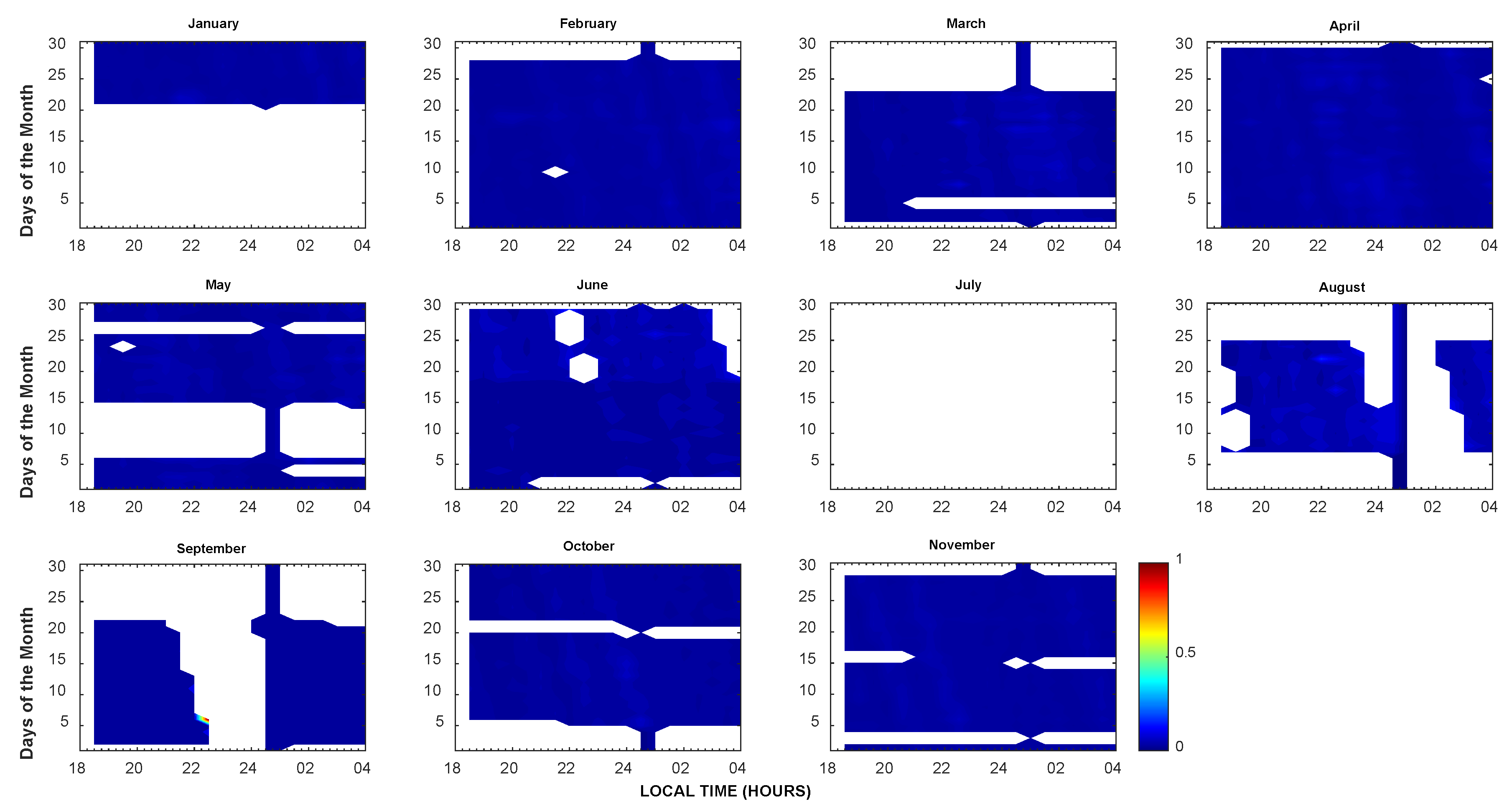
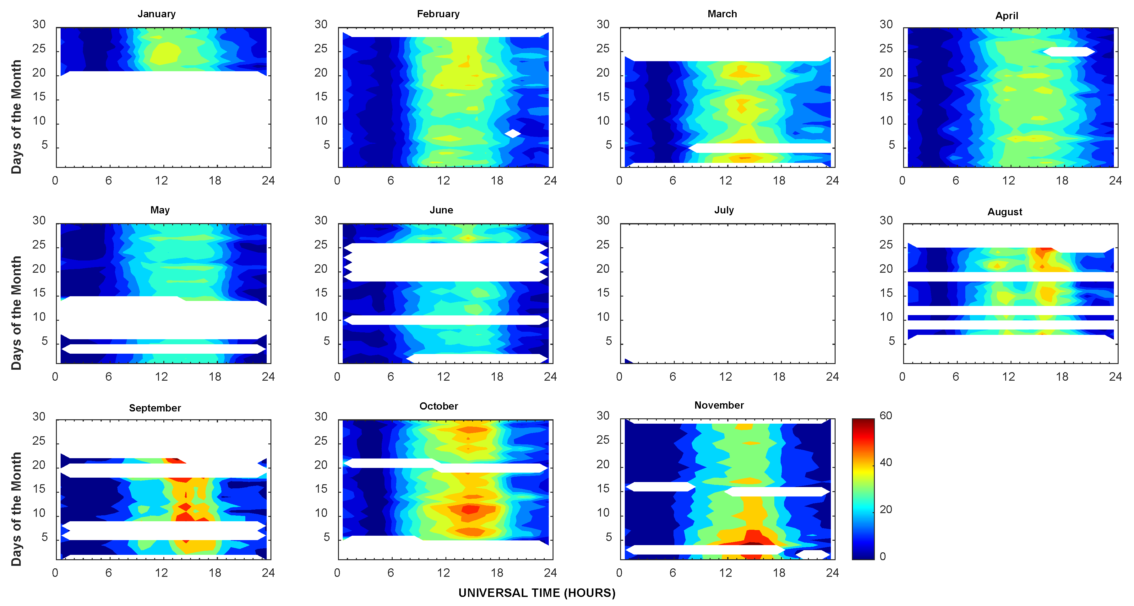
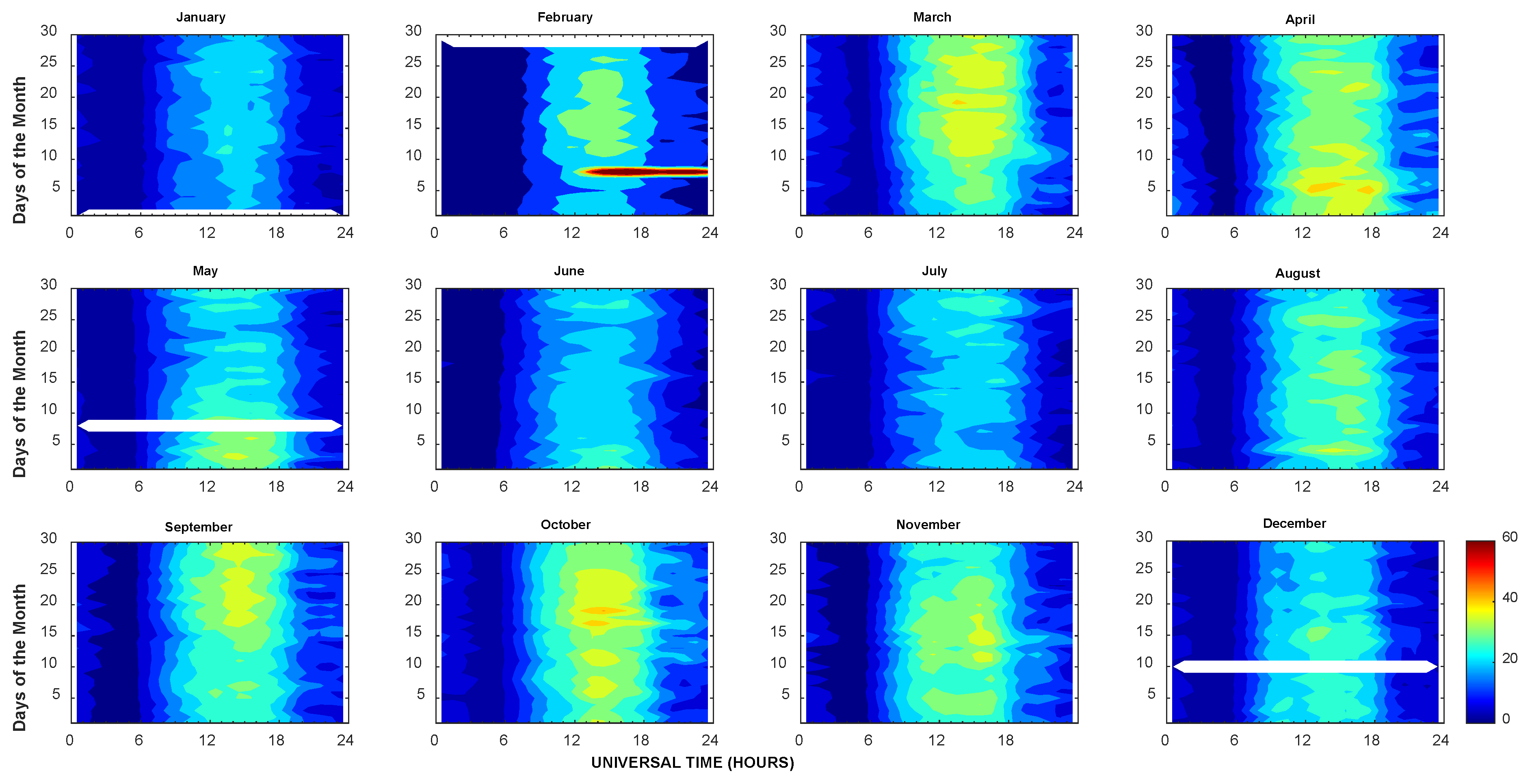
Figure 4 showed the results from our analysis concerning ROTI, which is calculated from the time variation in TEC (rate of change of TEC, ROT).
4. Results and Discussion
Figure 4 and
Figure 5 show the first results of the monthly TEC and ROTI observations from the CASES GPS receiver installed at Bowen University, Iwo, Osun State. The x and y axes of the contour plots show the days of the month and the universal time, respectively. The unfilled (white background) points represent unavailable data points due to unknown sources. Unavailable data points can be due to electric power supply or instrument errors which cannot be corrected during the CASES GPS’s recording.
The monthly TEC from the GPS data, as described in the methodology, has been computed for all months in 2021, a low-solar-activity year. These monthly observations are shown in
Figure 5 from January to November 2021. The right-handed bar shows the intensity of the monthly TEC. The monthly TEC is characterized by a minimum in magnitude at pre-sunrise (04:00 LT–06:00 LT, ~4 TECU–~5 TECU), maximum in magnitude at daytime (11:00 LT–15:00 LT, ~30 TECU–~50 TECU), decrease in magnitude at post-sunset (17:00 LT–20:00 LT, (~25 TECU–~35 TECU), and a further decrease at nighttime (20:00 LT–24:00 LT, ~7 TECU–~15 TECU).
Our observations agree with the previous investigations of [
1,
22,
23,
24,
25,
26,
27]. They reported the weakest TEC during the pre-sunrise hours. Around the equatorial station, they reported maximum TEC during the daytime, which was associated with the greater ionization of electrons due to the solar extreme ultra-violet (EUV) production, coupled with the upward vertical E X B drift [
1,
22,
23,
27,
28,
29].
According to references [
24,
30,
31], the decrease in TEC magnitude at post-sunset and nighttime hours is mostly due to the cessation of solar EUV production. This is in combination with the downward E x B drift velocity that lowers the ionosphere to an altitude where chemical losses are larger.
In comparison to the year 2021, a low-solar-activity period having a solar flux of ~82 sfu, is the year 2010, having a closer solar flux unit of 80. References [
32,
33] reported a minimum and maximum TEC magnitude at the June solstice and September equinox, respectively. Generally, the increase in electrons in the ionosphere is majorly controlled by solar flux production (photoionization) and recombination processes [
33,
34,
35]. Therefore, plasma is expected to be higher around the geomagnetic equator during the equinoctial months due to the abundance of the peak photoelectron and intense eastward electric field within the subsolar region. The plasma at the equator, associated with a decrease in photoelectron peaks during the solstice months, is due to the movement of the subsolar point to higher latitudes. In addition, we observed a semi-annual variation characterized by two maxima in equinoctial months. As reported by [
30], this was associated with the combined effect of zenith angle and magnetic field geometry.
All of these results from CASES GPS that compared well with other literature reports are good indicators as they confirm that the CASES GPS receiver at Bowen University has the required potential and capacity to capture reliable information about the varying equatorial ionosphere over Nigeria at any point in time.
Figure 4 displays the monthly variations in the ROTI. Similar to the TEC data in
Figure 5, the white background in
Figure 4 reaffirms the missing TEC data points. Our observations over all months show total suppression of irregularities. The suppression of these ionospheric irregularities may be ascribed to the decrease in the zonal neutral wind which was unable to generate the F-region dynamo near the sunset.
In order to further validate our results, we compared the TEC and ROTI measurements at BJCO with our results. Both results showed similar monthly TEC characterized by a diurnal pattern having a minimum pre-sunrise and a maximum daytime, post-sunset, and midnight decrease. Another conspicuous feature that is evident in
Figure 5 is the value of TEC at the BJCO, which is close to that of our observations. For instance, we observed 40 TECU, 45 TECU, and ~45 TECU compared to 45 TECU, 45 TECU, and ~50 TECU in September, October, and December at BJCO and Bowen, respectively. These disparities in the TEC values between both GPS stations can be traced to the annual solar flux index playing a primary role and having a value of ~82 sfu and ~80 sfu in 2021 and 2010, respectively. The longitudinal effect may not be significant in the varying TEC value between BJCO and Bowen. This is due to their longitudes, which are closer as BJCO is located at 4.14° E and Bowen is at 2.45° E. For clarity, the difference in local time due to the longitude where each of the GPSs are located is less than one hour. For example, the calculated local time (LT) at BJCO when the universal time (UT) is zero is 0.276. In the case of the Bowen location, it is 0.163. Therefore, the difference between both LT is 0.113. This value is smaller and may not have a significant impact on the varying TEC between both GPS locations. However, it may play a secondary role. It is important to note that both 2010 and 2021 are characterized by periods of low solar activity and belong to solar cycle 24. It is also important to note that the solar cycle effect is negligible for both years. Therefore, this difference in TEC magnitude may be due to the combined effect of the longitudinal difference and the solar flux index modification (
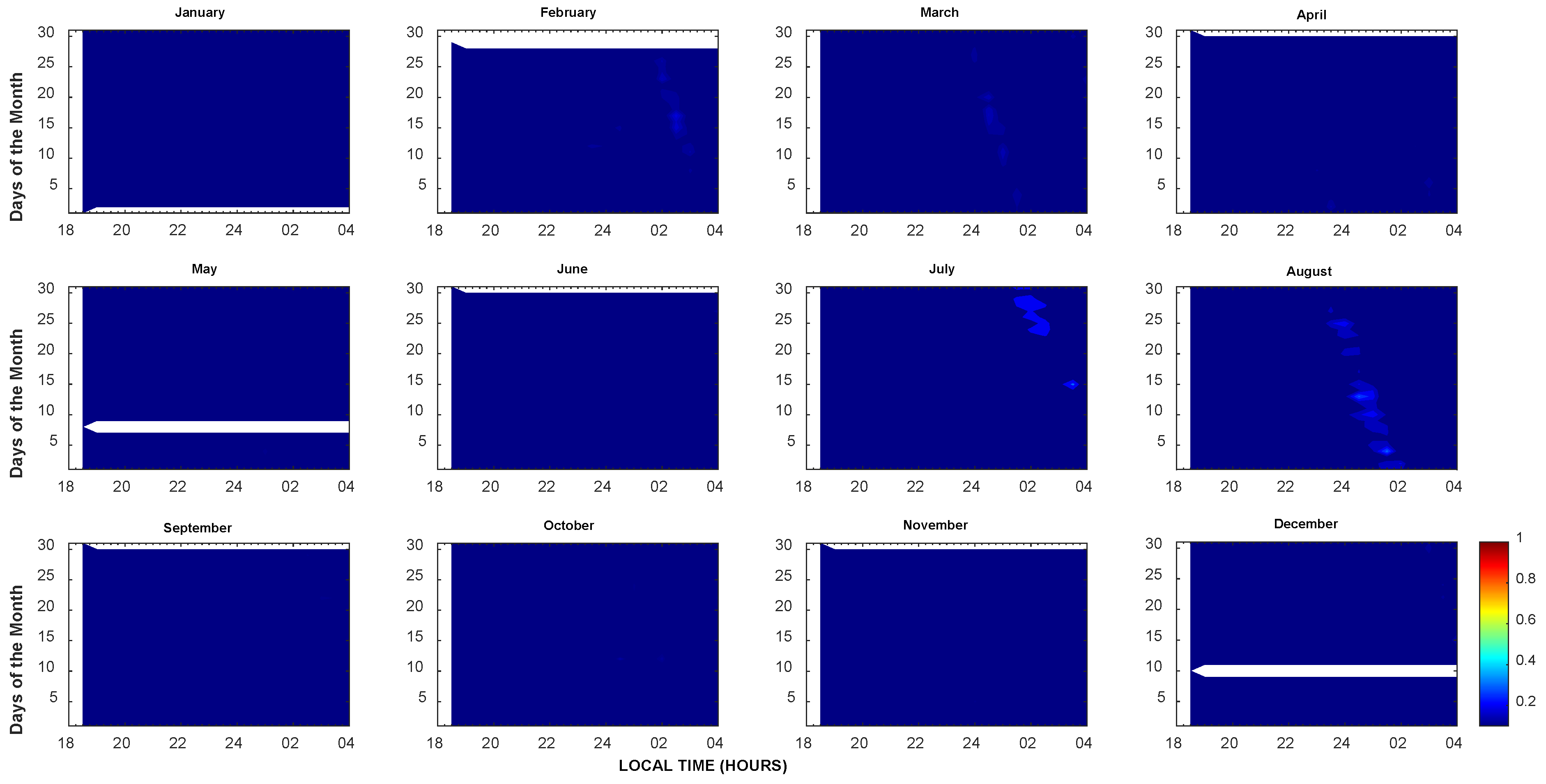
Figure 6). In addition,
Figure 7 displayed good agreement with the total suppression of ionospheric irregularities observed at BJCO when compared to Bowen.
The comparisons of ROTI results from both stations confirm similarities in their variability. These indicate that a CASES GPS receiver located at Bowen has similar capacities and reliability as that at BJCO. Therefore, it can now be known how ionospheric irregularities over the Nigerian ionosphere affect our technologies related to navigation and positioning.

 ,
, 


