

Odour Emissions and Dispersion from Digestate Spreading

 , , and
Abstract
:1. Introduction
2. Materials and Methods
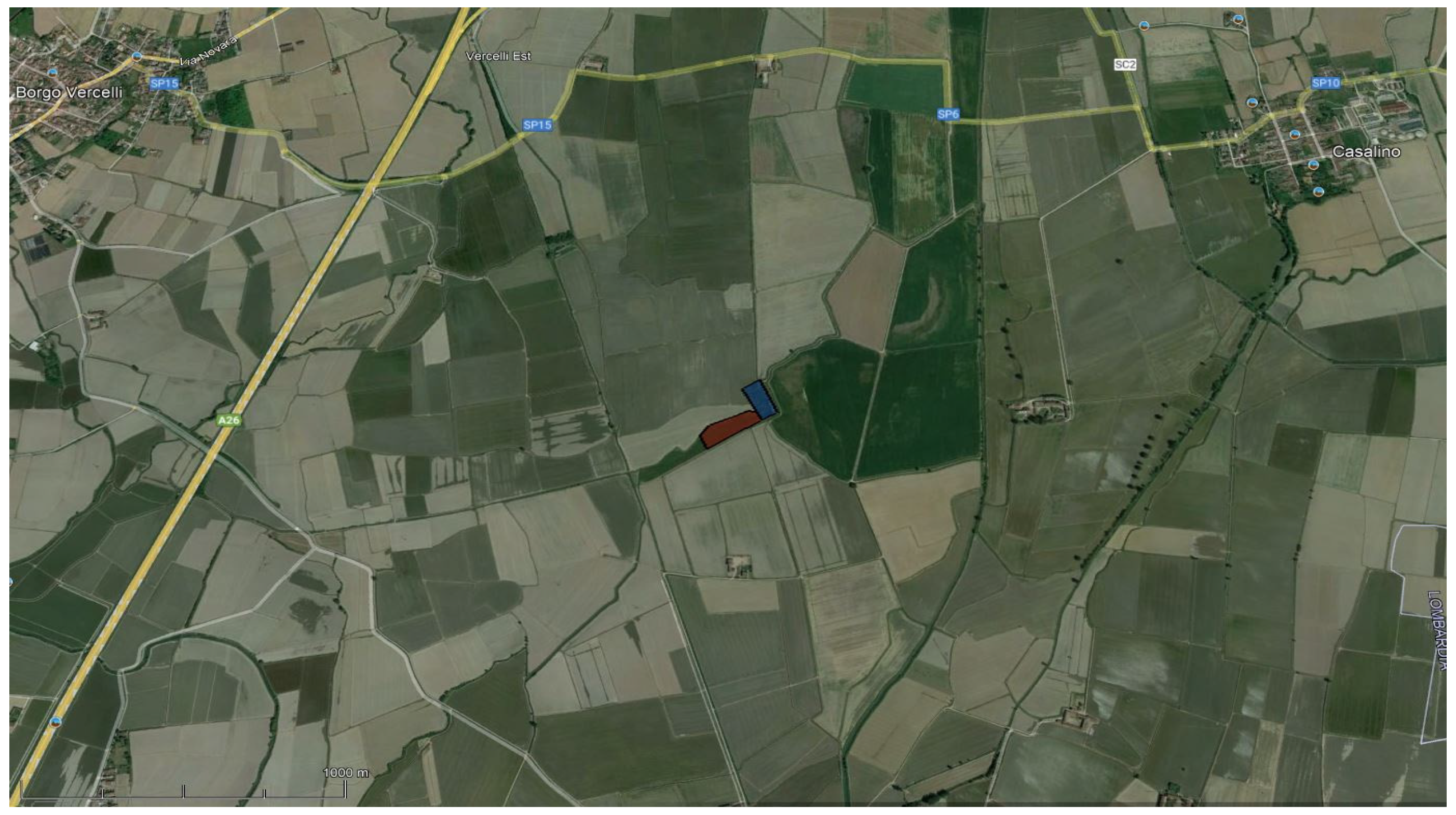
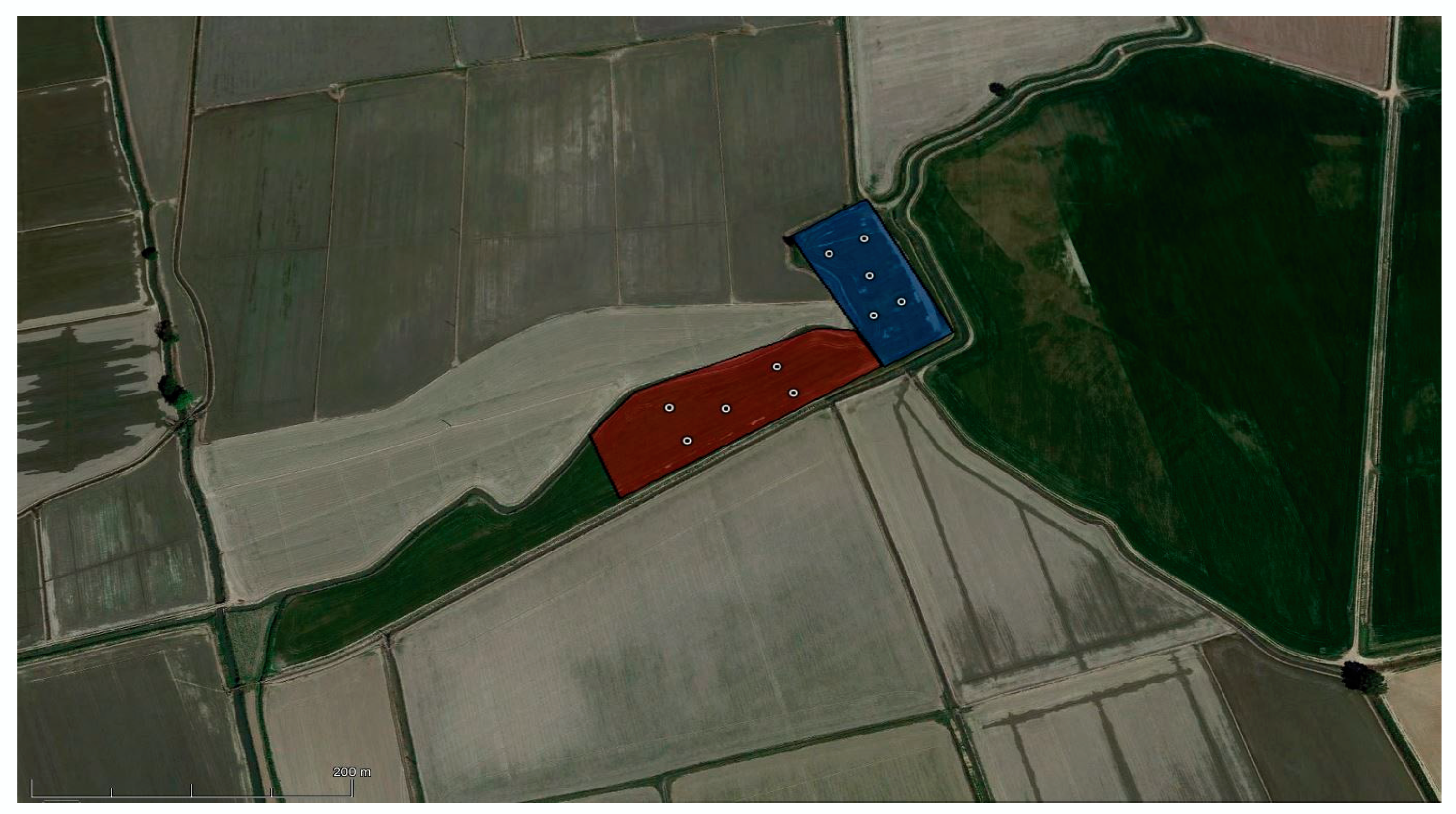
2.1. The Experimental Site
2.2. Odour Measurements
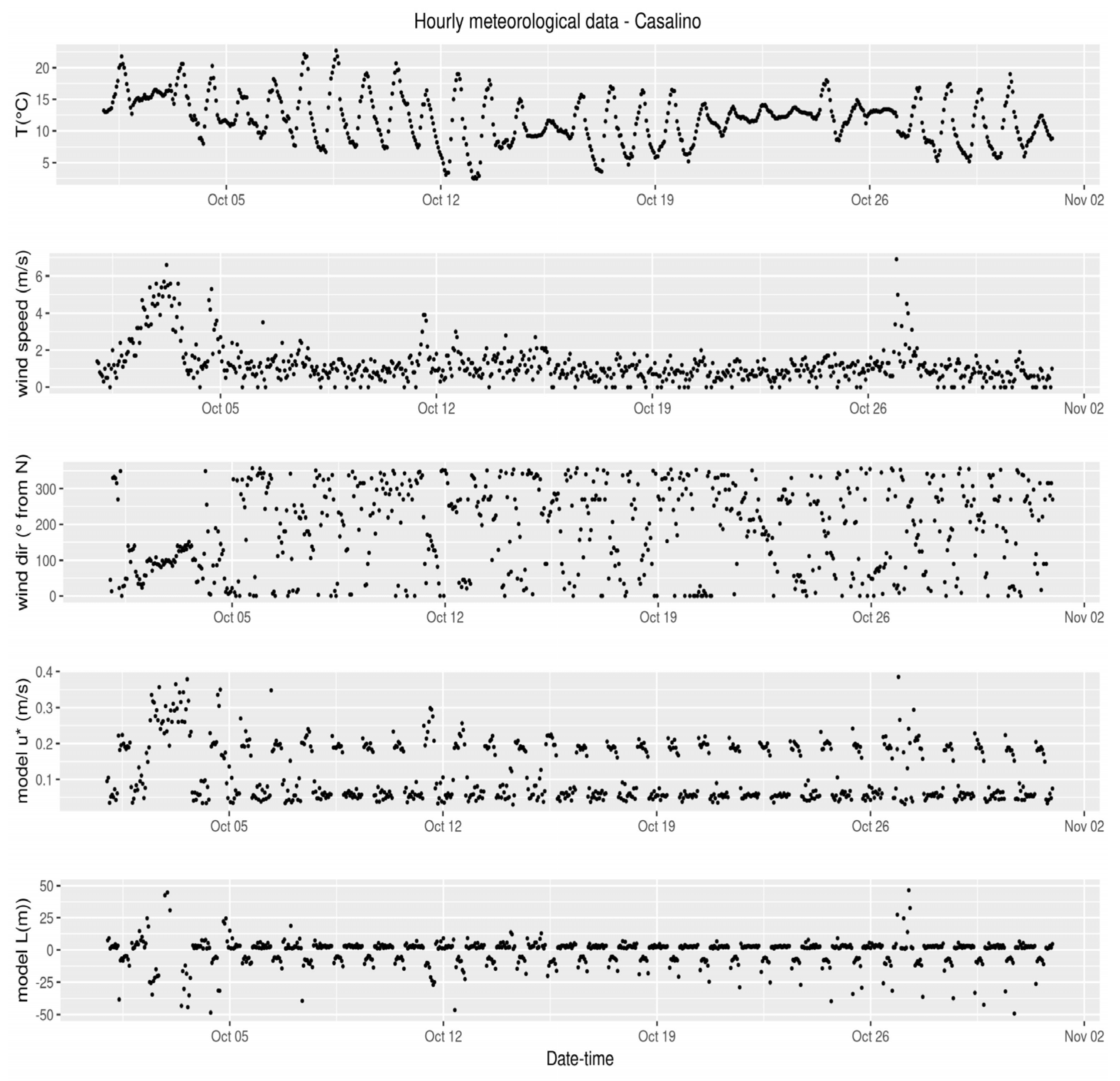
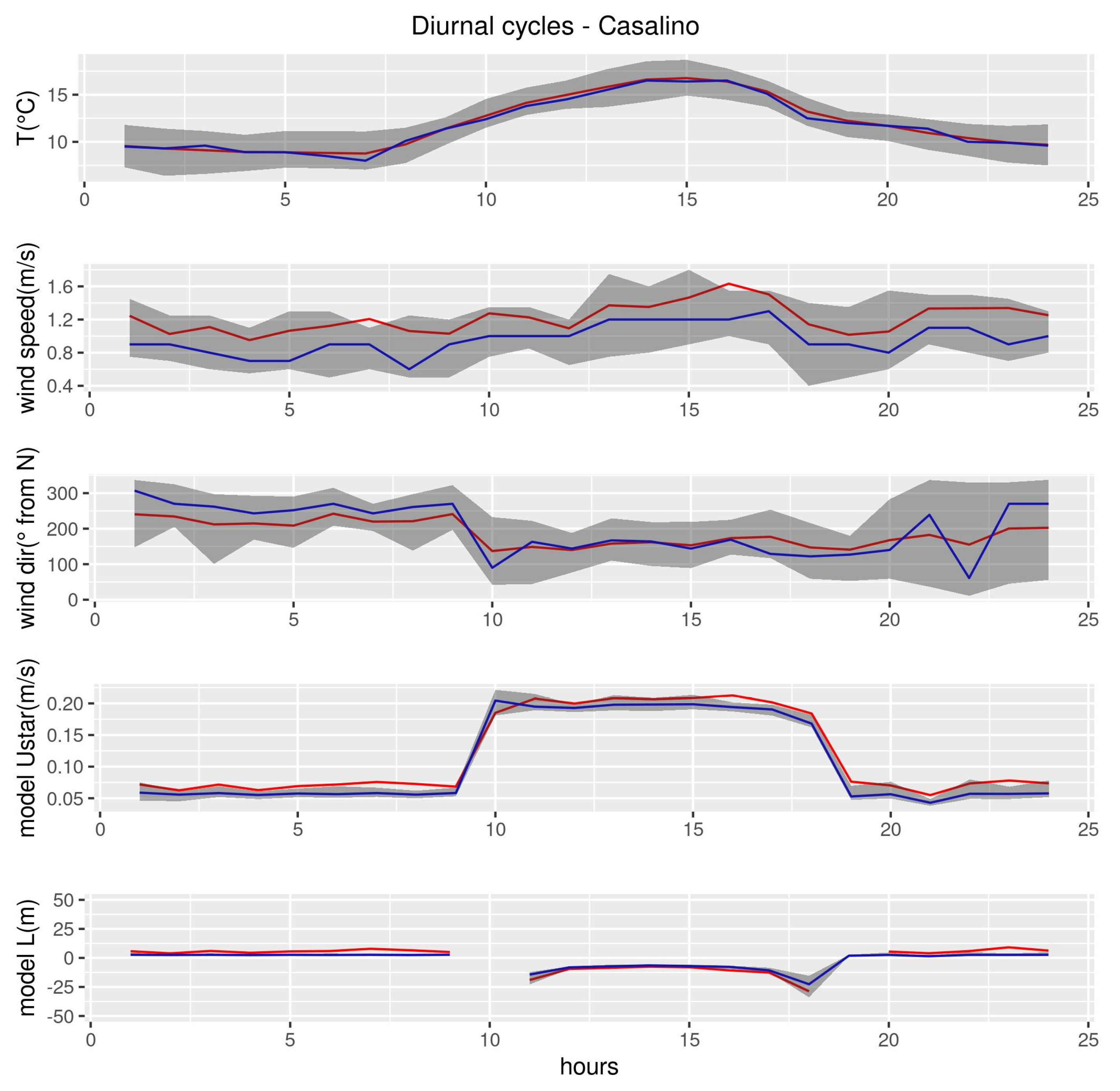
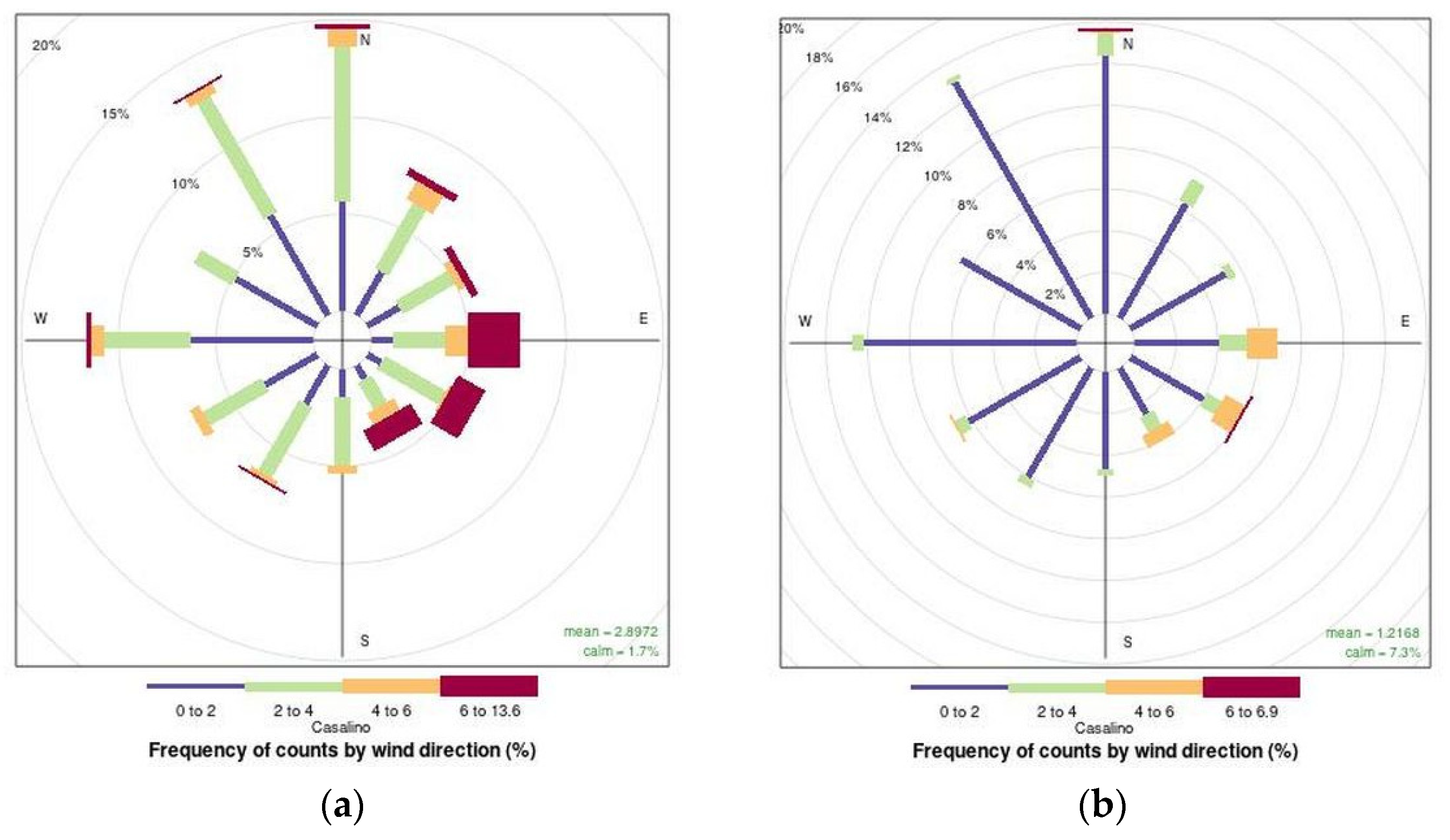
2.3. Meteorological Measurements
2.4. Odour Dispersion Modeling
2.4.1. The Selected SCICHEM Model
- In line with the Italian regulations, particularly that of the Lombardy Region that commissioned the study [20].
- In line with the standard UNI 10796:2000 that specified the classes of the models that are recommended as applicable to the problem of odour nuisances (i.e., non-stationary puff models/segment models, 3D Lagrangian puff or particle models, 3D Eulerian models).
- Spatial and temporal scales compatible with the problem under analysis.
- Transport and turbulent schemes adequately representing the peculiarities of odour dispersion.
- Able to represent the aerodynamic effect and mitigation potential of the barriers.
- Able to represent the inhomogeneous surfaces and the effects of canopies.
- Actively used and maintained by the scientific community, multi-platform and open source.
- User friendly and with low–moderate computational resources requirements for easy use in non-academic contexts (e.g., administrative/regulatory).
- Mean wind (intensity and direction)
- Wind gust (intensity and direction)
- Air temperature
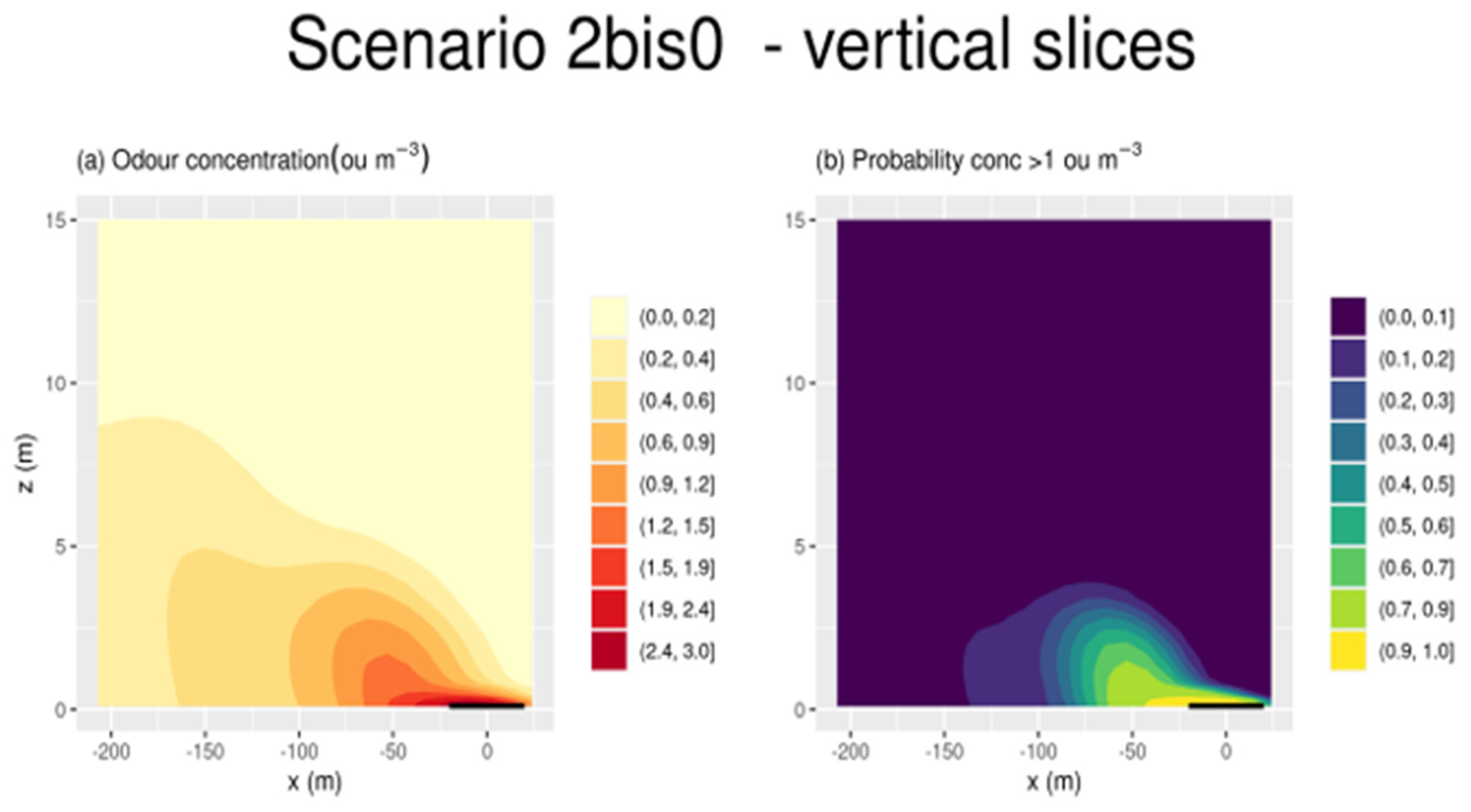
2.4.2. Selected Simulation Scenarios
- The diameter of the point source was set as large as possible (40 m diameter, about 0.1 ha), compatibly with numerical stability.
- The height of the point source was set to zero.
- The ejection velocity and buoyancy effects, typical of a point/stack source, were set to zero as the field was a passive source.
- The total emission value was set equal to that of scenario 2.
- The meteorological data were those of the wind gust event occurring in scenario 2.
- The mass effects (inertia, gravity) of the transported quantity were not considered.
- The chemical reactions were not considered.
- The deposition was switched off.
- The surface roughness length was set to 0.01 m (rough, bare soil).
- The maximum number of receptors allowed by the model is 500, therefore, we set a grid of 22 × 22 equally spaced receptors across the domain.
- The output time step was set to 15 min.
3. Results
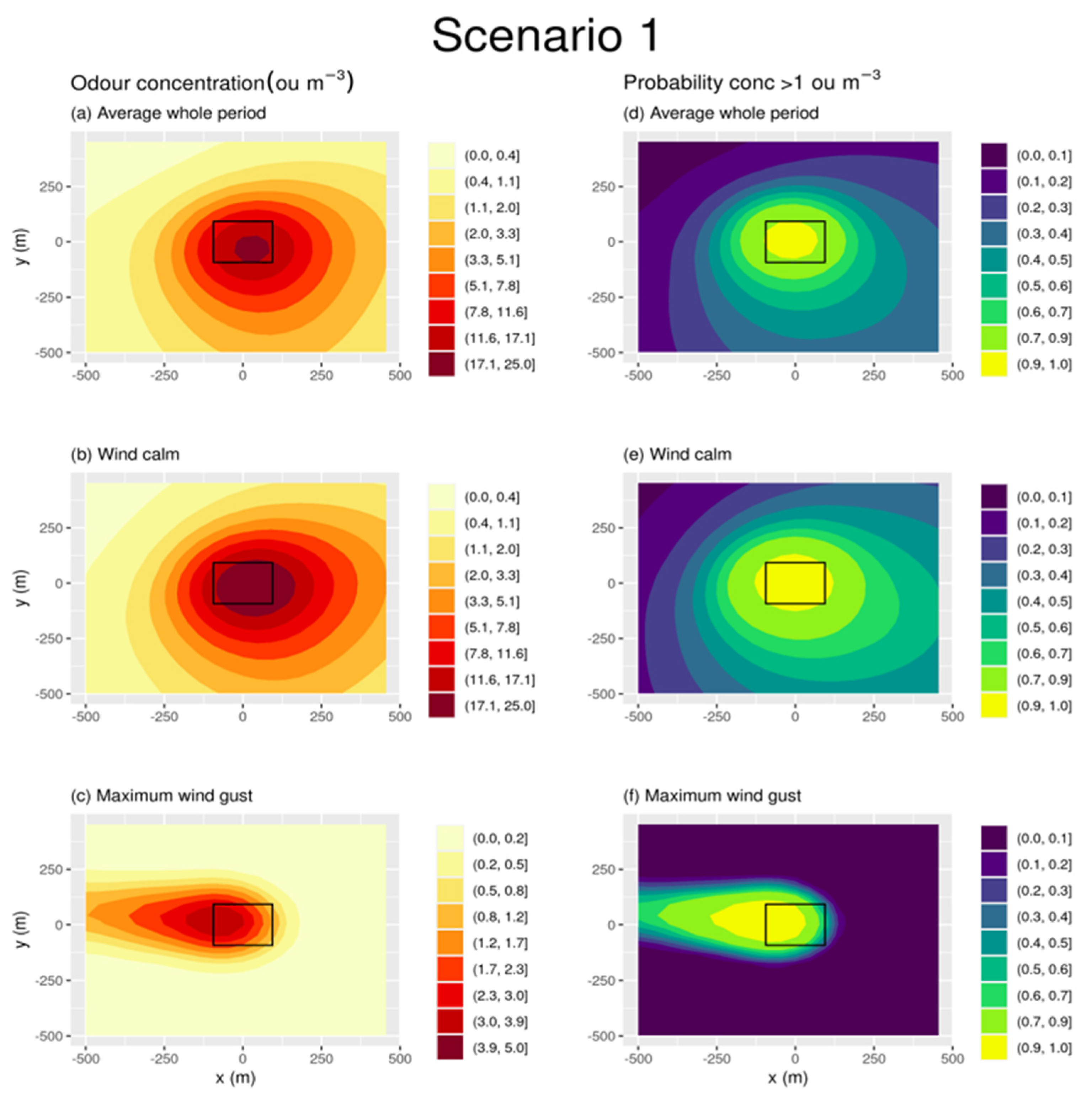
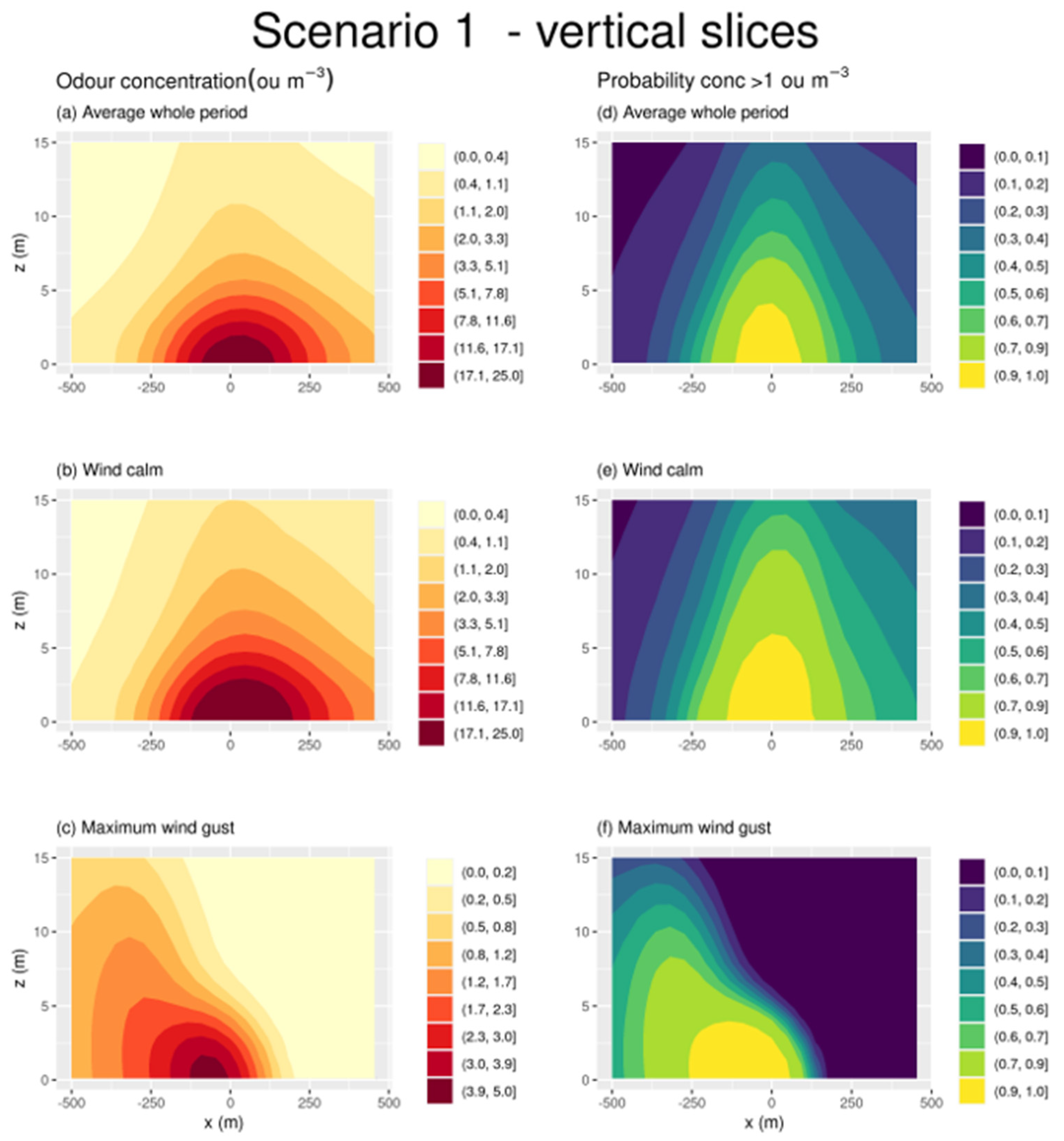
3.1. Modeled Odour Concentration Plume
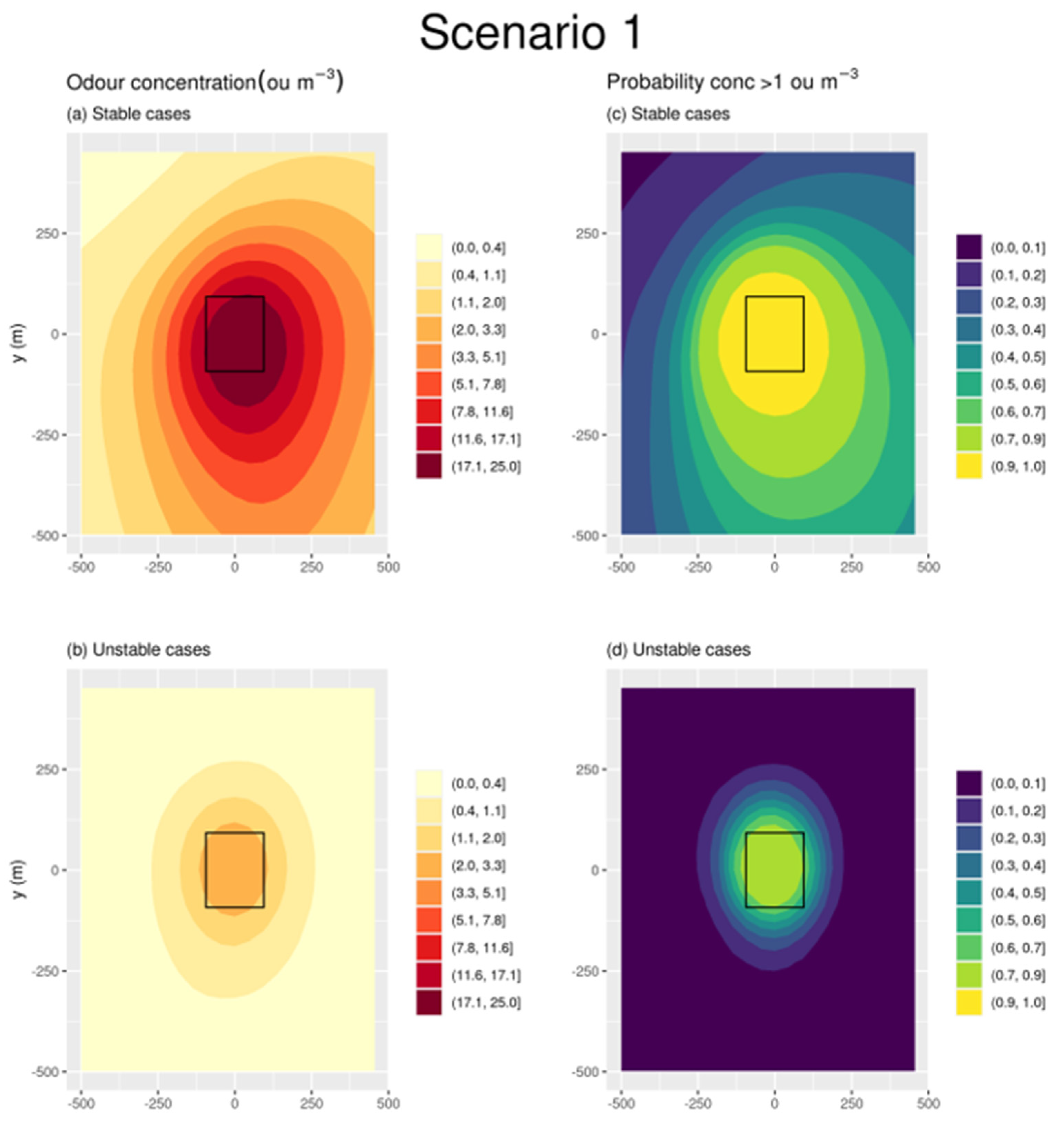
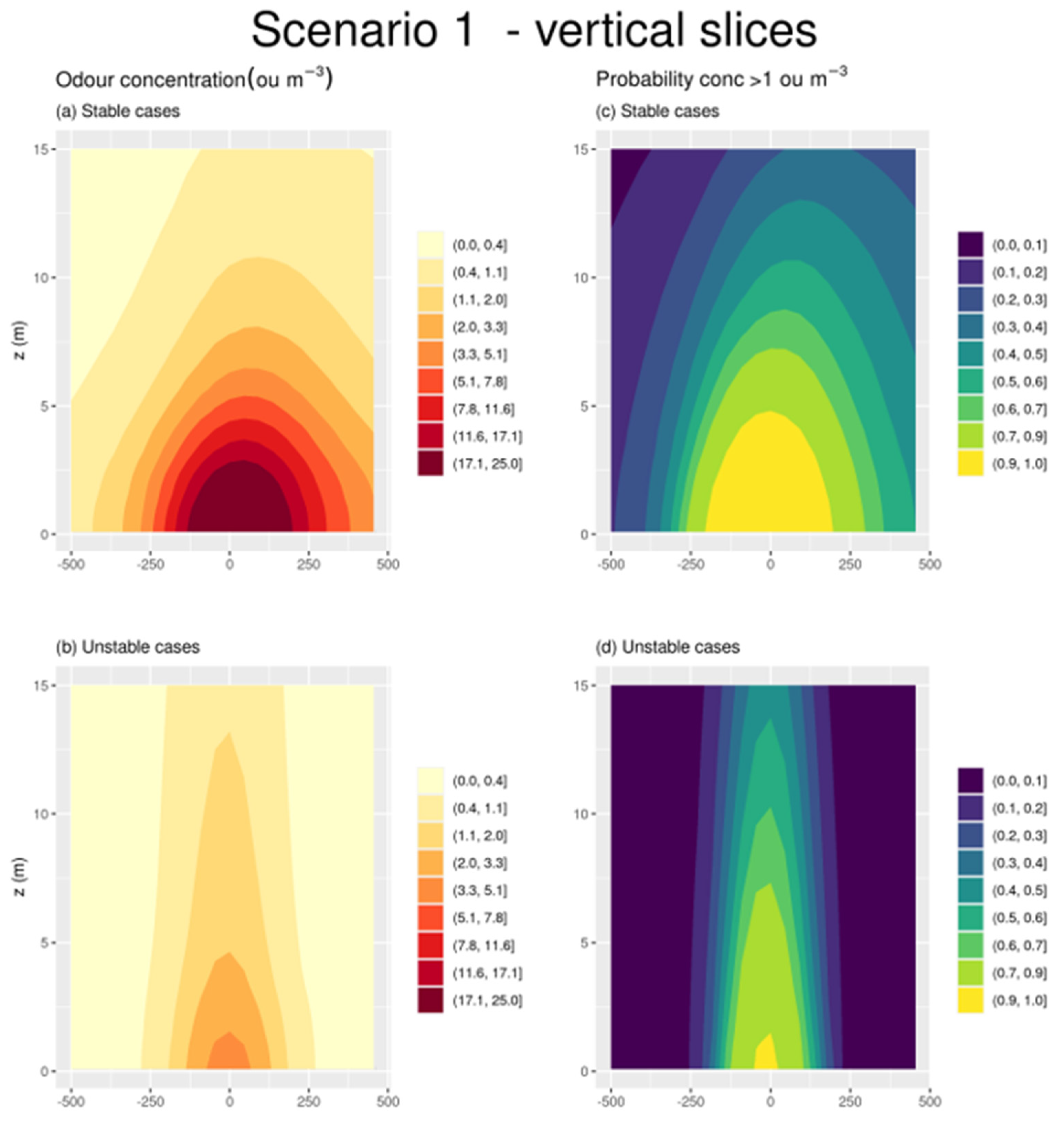
3.2. Effect of Stability
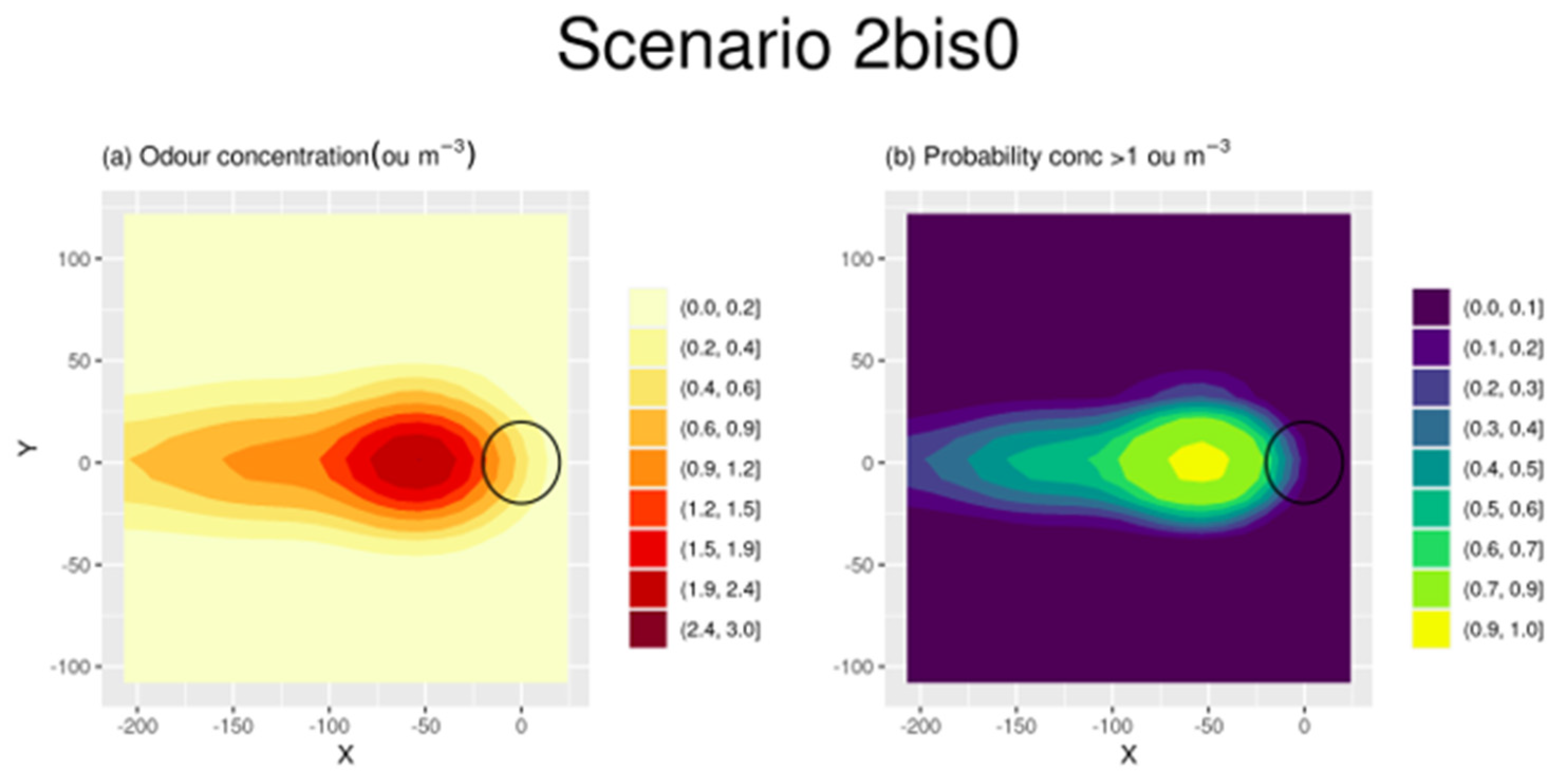
3.3. Effect of Reduced Emissions
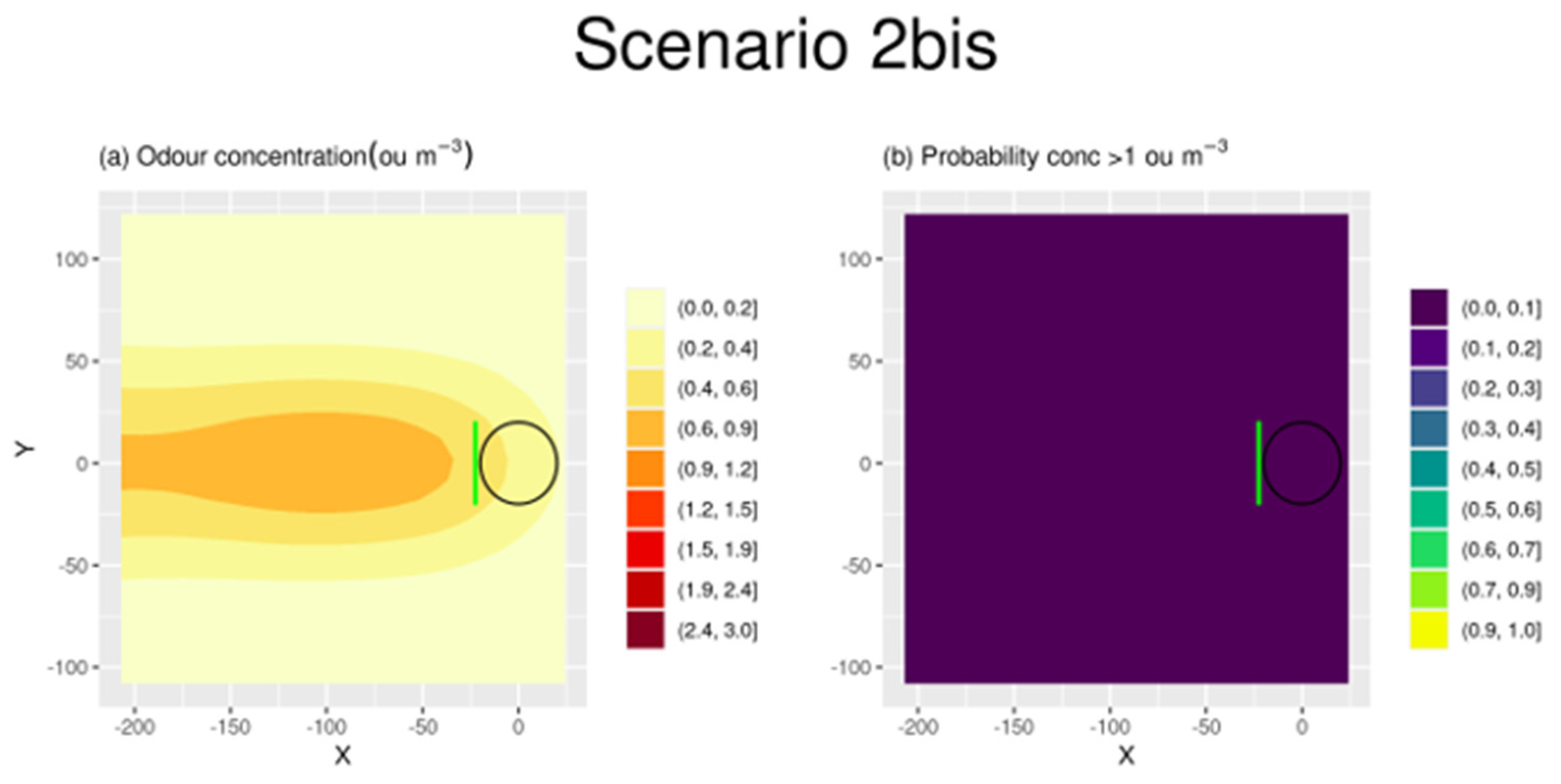
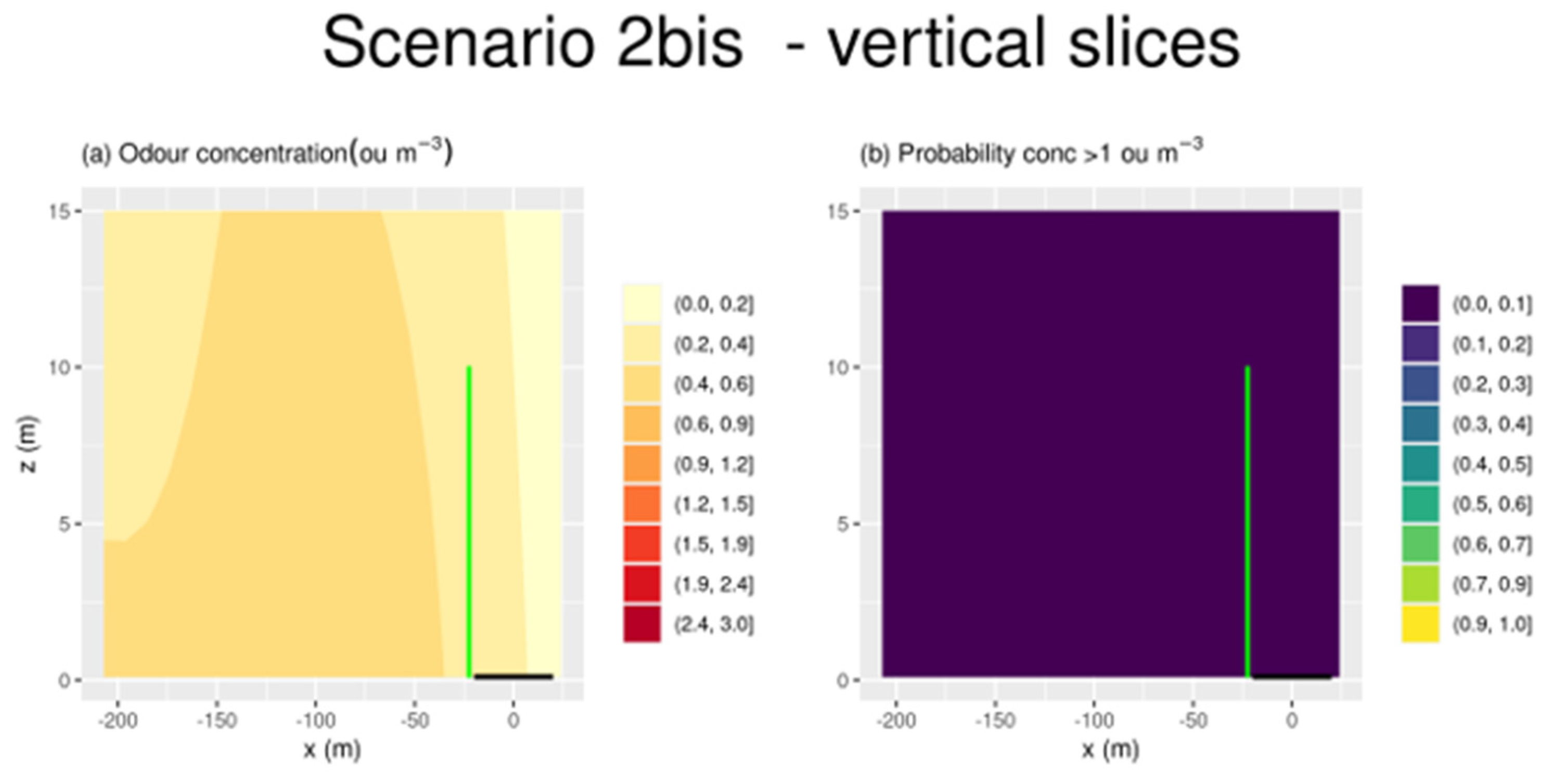
3.4. Effect of Barriers
4. Conclusions
- The chosen threshold was the lowest considered by the Italian regulation.
- The emissions was considered constant during the whole month, thus constituting a “worst-case scenario” where fertilizer applications are either replicated very frequently or performed in neighbors’ fields almost at the same time and for an extended period.
Author Contributions
Funding
Institutional Review Board Statement
Informed Consent Statement
Data Availability Statement
Acknowledgments
Conflicts of Interest
Appendix A

| Parameter | Value |
|---|---|
| Ammonia nitrogen (g/kg) | 2.97 |
| Total nitrogen (g/kg) | 4.50 |
| TAN (total ammonia nitrogen)/TKN (Total Kjeldahl Nitrogen) (%) | 66.00 |
| pH | 7.30 |
| Total phosphorus (g/kg) | 2.35 |
| Total potassium (g/kg) | 3.05 |
| Parameter | Value |
|---|---|
| m3 /ha applied | 40.0 |
| N applied (kg/ha) | 180.0 |
| N-NH3 applied (kg/ha) | 118.8 |
Appendix B
- Representation of transport
- 2.
- Possibility to model dispersion over complex terrain
- 3.
- Possibility to model dispersion across obstacles
- 4.
- Possibility to model dry and wet deposition
- 5.
- Possibility to model chemical reactions and radioactive decay
- 6.
- Specific for odours or designed for tracers but applicable to odours
- -
- -
- Peak-to-mean schemes (applicable to both the plume and Lagrangian models).
- 7.
- Type of source that can be modeled
- 8.
- Spatial scale of applicability
- 9.
- Time step and averaging interval
- 10.
- Applied in regulatory context
- 11.
- License
- 12.
- Existence of a user manual, graphical user interface, and technical documentation
Appendix B.1. Steady-State Plume Models
Appendix B.1.1. AERMOD
- Representation of transport: Convective and stable conditions are represented by different parametrizations of micrometerological parameters (L, u*, w*) and stability functions. The wind profile is assumed to be logarithmic. The pollutant plume is represented by Gaussian functions. In the CBL (convective boundary layer), the plume is represented as bi-Gaussian in z (vertical dispersion) and Gaussian in y (horizontal dispersion). In the SBL, both the horizontal and vertical shapes are assumed to be Gaussian. The pollutant plume is the weighted sum of a “horizontal plume” (terrain impacting) and a “terrain following” plume.
- Possibility to model dispersion over complex terrain: Yes.
- Possibility to model dispersion across obstacles: AERMOD can represent the effect of building wakes on the plumes through the incorporation of the PRIME algorithm (plume rise model enhancements).
- Possibility to model dry and wet deposition: Yes.
- Possibility to model chemical reactions and radioactive decay: Radioactive decay only.
- Type of source that can be modeled: AERMOD can handle point, line, area, and volume sources, eventually with buoyancy effects.
- Spatial scale of applicability: As most of the steady-state Gaussian models, AERMOD assumes the homogeneous properties of the flow across the modeling domain. Therefore, the spatial scale of applicability is of a few km.
- Time step and integration interval: Minimum sampling interval is one hour.
- Applied in regulatory context: AERMOD was formulated and has been widely used in regulatory contexts, being the reference U.S. Environmental Protection Agency regulatory model [61].
- License: Software is available at no cost.
- Existence of a user manual, graphical user interface, and technical documentation: Yes. Website: https://www.epa.gov/scram/air-quality-dispersion-modeling-preferred-and-recommended-models#aermod (URL accessed on 14 February 2023)
Appendix B.1.2. ADMS
- Representation of transport: Convective and stable conditions are represented by different parametrizations of micrometerological parameters (L, u*, w*), and stability functions. The pollutant plume is represented by Gaussian functions and skewed distributions in the CBL. The effects of the buoyant plume rise can be modeled. The ADMS also includes a “puff” module.
- Possibility to model dispersion over complex terrain: Yes.
- Possibility to model dispersion across obstacles: Yes.
- Possibility to model dry and wet deposition: Yes.
- Possibility to model chemical reactions and radioactive decay: Yes.
- Type of source that can be modeled: ADMS can handle point, line, area, and volume sources.
- Spatial scale of applicability: Different versions of the model exist, optimized for various contexts and spatial scales (ADMS-Roads, ADMS-Urban, ADMS-Airport). The maximum spatial scale is limited by the hypothesis of the horizontal homogeneity. It is, therefore, limited to the short range, i.e., a few km. Nevertheless, a specific version of the model has been developed for nesting the ADMS to regional models (ADMS-Urban regional model).
- Time step and averaging interval: Integration time interval is 1 h.
- Applied in regulatory context: ADMS is widely used in regulatory contexts (e.g., UK Health and Safethy Executive, Environment Agency in England, Scottish Environmental Protection Agency, Northern Ireland Environment Agency, Natural Resources Wales, Food Standards Agency of the United Kingdom).
- License: Proprietary, charges on distribution.
- Existence of a user manual, graphical user interface, and technical documentation: Yes. Website: https://www.cerc.co.uk/environmental-software/ADMS-model.html (URL accessed on 14 February 2023)
Appendix B.1.3. CDTMPLUS
- Representation of transport: The pollutant plume is represented by Gaussian functions. In the CBL (convective boundary layer), the plume is represented as skewed, bi-Gaussian in z (vertical dispersion), and Gaussian in y (horizontal dispersion). In the SBL, both the horizontal and vertical shapes are assumed to be Gaussian. The effects such as the buoyant or mechanical plume rise can be modeled, as well as the partial plume penetration into elevated stable layers.
- Possibility to model dispersion over complex terrain: The effects of very complex terrains can be modeled with a dedicated preprocessor which needs a 3D description of the terrain as the input.
- Possibility to model dispersion across obstacles: Yes.
- Possibility to model dry and wet deposition: Yes.
- Possibility to model chemical reactions and radioactive decay: No.
- Specific for odours or designed for tracers but applicable to odours: No reference was found about use of CDTMPLUS for odours.
- Type of source that can be modeled: Only point.
- Spatial scale of applicability: Short range (< 5 km).
- Time step and averaging interval: Integration time step 1 h.
- Applied in regulatory context: CDTMPLUS has been widely used in regulatory contexts and is listed among the “preferred and recommended models” of the U.S. Environmental Protection Agency [27] for air quality dispersion modeling.
- License: Software is available at no cost.
- Existence of a user manual, graphical user interface, and technical documentation: Yes. Website: https://www.epa.gov/scram/air-quality-dispersion-modeling-preferred-and-recommended-models#ctdmplus (URL accessed on 14 February 2023)
Appendix B.1.4. FIDES
- Representation of transport: The functional form of the plume is taken from [66], a variant of the classical Gaussian shape, and the wind profiles are assumed to follow a power law. The meteorological data in the input (hourly time step) include the wind direction, roughness length z0, Obukhov length L, and friction velocity u*. L, z0, and u* can be either given as the input or calculated by the model from the wind, temperature, and canopy height data.
- Possibility to model dispersion over complex terrain: No.
- Possibility to model dispersion across obstacles: No.
- Possibility to model dry and wet deposition: Yes.
- Possibility to model chemical reactions and radioactive decay: No.
- Specific for odours or designed for tracers but applicable to odours: No reference was found about use of FIDES for odours.
- Type of source that can be modeled: Point, line, area, and volume sources, continuous and discontinuous.
- Spatial scale of applicability: local scale, < 5 km.
- Time step and averaging interval: The integration time is 30 min.
- Applied in regulatory context: No reference was found about use of FIDES in regulatory contexts.
- License: The FIDES software is distributed at no cost.
- Existence of a user manual, graphical user interface, and technical documentation: The model can be used with the following languages: visual basic, R, Matlab, and C, but no dedicated GUI is available. A succinct user manual is available. Website: https://www6.versailles-grignon.inrae.fr/ecosys_eng/Productions/Softwares-Models/FIDES2 (URL accessed on 14 February 2023)
Appendix B.1.5. OdiGauss
- Representation of transport: OdiGauss is a steady-state Gaussian plume model, implementing [68] parametrizations for the plume functional form and dispersion coefficients. It accounts for the atmospheric stability through the Pasquill classes, and for calm wind (wind speed <0.5 m/s) with a dedicated algorithm, similar to the ISCST3 model or the Cirillo–Poli model [69].
- Possibility to model dispersion over complex terrain: No.
- Possibility to model dispersion across obstacles: No.
- Possibility to model dry and wet deposition: A corrective coefficient is applied in the occurrence of rain to consider the phenomenon of odour removal due to “scavenging”.
- Possibility to model chemical reactions and radioactive decay: No.
- Specific for odours or designed for tracers but applicable to odours: The model OdiGauss has been specifically designed for odours, implementing a peak-to-mean correction to the average output concentrations. A constant value of the peak-to-mean ratio is adopted, which may be tuned to follow a precautionary criterion. The suggested default value is equal to 2.3, while a value of one disables the peak-to-mean correction.
- Type of source that can be modeled: The model can either ingest constant emission rates, or variable, multiple, and more complex emissions as modeled by the EmiFarm model, also included in the OdiGauss package. EmiFarm simulates odour emissions from poultry manure heaps.
- Spatial scale of applicability: Short range (<5 km).
- Time step and averaging interval: Integration period is one hour.
- Applied in regulatory context: Applied in the context of environmental authorization procedures (e.g., [70]).
- License (proprietary—charges on distribution/ proprietary—distributed at no cost/open source): Software publicly available at no cost.
- Existence of a user manual, graphical user interface, and technical documentation: Yes. Website: http://semola.uniud.it/projects/odigauss/ (URL accessed on 13 February 2022)
Appendix B.2. Lagrangian Models
Appendix B.2.1. WindTrax
- Representation of transport:
- 2.
- Possibility to model dispersion over complex terrain: No.
- 3.
- Possibility to model dispersion across obstacles: No.
- 4.
- Possibility to model dry and wet deposition: No, the surface is assumed to be reflective. In a Lagrangian model, this means that particle trajectories intersecting the surface are “reflected” back into the flow. A version of the software with deposition has also been developed, but at present it is used for research purposes and not publicly available.
- 5.
- Possibility to model chemical reactions and radioactive decay: No.
- 6.
- Specific for odours or designed for tracers but applicable to odours: Windtrax does not include specific modules for odours, but has been applied in this context either by using methane as a tracer and indicator of the odour concentration [75] or directly simulating the odour concentrations in ou/m³ [76].
- 7.
- Type of source that can be modeled: Point, line, area, and volume sources can be modeled. Non-steady emissions can be handled if the timescales of their variations is longer than the model integration period (30 min).
- 8.
- Spatial scale of applicability: The WindTrax model is a short-range model, applicable to distances less than approximately 5 km from a gas source. It is a surface layer model and errors can be expected at larger downwind distances as (1) trajectories may travel above the surface layer and then descend back into the surface layer, (2) assumptions of horizontal homogeneity of the wind may be violated, and (3) assumptions of stationarity in the wind can be violated.
- 9.
- Time step and averaging interval: The model averaging time is generally set between 10 and 60 min, meaning that the meteorological and emission data should be provided at this frequency, and the output concentration will be averaged on this time interval. The internal model timestep (for solving the Langevin equations) is instead specified as a certain fraction of the Lagrangian time scale (typically <1 s) and is calculated according to the flow characteristics [74].
- 10.
- Applied in regulatory context: WindTrax has been accepted for regulatory reporting purposes. T.K. Flesch (personal communication) reports that WindTrax has been used in Canada for regulatory reporting of methane and carbon dioxide emissions from industry.
- 11.
- License: WindTrax is a proprietary software (Thunder Beach Scientific) but freely available and distributed at no cost.
- 12.
- Existence of a user interface and manual (y/n): Yes. Website: http://www.thunderbeachscientific.com/ (URL accessed on 14 February 2023)
Appendix B.2.2. SPRAY
- Representation of transport:. The model solves the Langevin equation to follow the trajectories of a certain number of particles released for each emission episode. The turbulent flow can be parametrized as Gaussian, with velocity fluctuations depending on the atmospheric stability, according to [68]. In addition, the model contains several schemes for considering non-Gaussian, skewed velocity distributions and non-stationary flows.
- 2.
- Possibility to model dispersion over complex terrain: Yes.
- 3.
- Possibility to model dispersion across obstacles: Yes, in the “microscale version” of the model (PSPRAY).
- 4.
- Possibility to model dry and wet deposition: Yes.
- 5.
- Possibility to model chemical reaction/radioactive decay: Only radioactive decay in the SPRAY version and simplified chemical mechnisms for NOx/NO2 transformation (PSPRAY version).
- 6.
- 7.
- Type of source that can be modeled: Point, line, area, and volume sources, continuous and discontinuous. Both passive and momentum or buoyancy forced emissions can be modeled.
- 8.
- Spatial scale of applicability, spatial resolution if applicable: From micro (1 km) to regional scales.
- 9.
- Time step: Both time step and integration interval are variable, depending on the meteorological and emission conditions.
- 10.
- 11.
- License: Proprietary.
- 12.
- Existence of a graphical user interface and manual: Yes. Website: https://www.aria-net.it/it/prodotti/spray/ (URL accessed on 14 February 2023)
Appendix B.2.3. FLEXPART
- Representation of transport: FLEXPART assumes a default underlying Gaussian turbulence and parametrizations of velocity fluctuations depending on the atmospheric stability, according to [68]. However, it contains options to switch to non-Gaussian, skewed velocity distributions [86]. The model handles deep convection by using the [87] scheme.
- Possibility to model dispersion over complex terrain: Yes.
- Possibility to model dispersion across obstacles: Yes.
- Possibility to model dry and wet deposition: Yes.
- Possibility to model chemical reaction/radioactive decay: Radioactive decay only.
- Specific for odours or designed for tracers but applicable to odours: FLEXPART was designed for gases and particles, but has also been used for odours in some specific applications (e.g., [88]).
- Type of source that can be modeled: Point, line, area, or volume sources can be modeled.
- Spatial scale of applicability, spatial resolution if applicable: Local to global, but more frequently used for mesoscale problems.
- Time step: Time step is variable, depending on the the flow conditions.
- Applied in regulatory context: FLEXPART has been widely used in regulatory contexts, including the reconstruction of the Chernobyl accident, and the estimation of halocarbon emissions (regulated by the Montreal Protocol).
- License: Publicly available and open source, released under the GNU General Public License.
- Existence of a user manual, graphical user interface, and technical documentation: Yes. Website: https://www.flexpart.eu/ (URL accessed on 14 February 2023)
Appendix B.2.4. HYSPLIT
- Representation of transport: HYSPLIT combines Lagrangian and Eulerian approaches by using of a moving frame of reference for the advection—diffusion calculations and a fixed three-dimensional grid as the frame of reference to compute the pollutant concentrations. The model can be used for simulating either particles or “puffs”, both in forward and backwards modes.
- Possibility to model dispersion over complex terrain: Yes, limited to what is resolved by the meteorological model’s terrain.
- Possibility to model dispersion across obstacles: No.
- Possibility to model dry and wet deposition: Yes.
- Possibility to model chemical reaction/radioactive decay: Yes.
- Type of source that can be modeled: Point and area sources, instantaneous or continuous.
- Spatial scale of applicability: Local to continental.
- Time step and averaging interval: Time step is variable, depending on the the flow conditions. Minimum value for the time step is 1 min.
- Applied in regulatory context: HYSPLIT has been used in several cases for regulatory purposes, for example in emergency response and the reconstruction of nuclear accidents, such as Chernobyl and Fukushima.
- License: HYSPLIT sowtware is publicly available and distributed at no cost.
- Existence of a user manual, graphical user interface, and technical documentation: Yes. Website: https://www.ready.noaa.gov/HYSPLIT.php (URL accessed on 14 February 2023)
Appendix B.2.5. AUSTAL2000
- Representation of transport: AUSTAL2000 is a stochastic Lagrangian dispersion model simulating particle trajectories by solving the Langevin equation and sampling them at the receptor location by using statistical techniques. The input data that are used by the model to represent the underlying flow include the roughness length, wind measurement height, wind direction, wind speed, and stability classes, according to Klug–Manier (analogous of the Pasquill stability classes).
- Possibility to model dispersion over complex terrain: Yes.
- Possibility to model dispersion across obstacles: Yes.
- Possibility to model dry and wet deposition: Dry deposition is handled.
- Possibility to model chemical reactions and radioactive decay: Yes.
- Specific for odours or designed for tracers but applicable to odours: AUSTAL2000 contains an aerosol module (peak-to-mean) for making predictions about the frequency of odour nuisance.
- Type of source that can be modeled: Point, line, area, and volume, constant or variable, with or without buoyant rise. Multiple sources can be handled by the model.
- Spatial scale of applicability: Up to 50 km.
- Time step and averaging interval: Variable time step according to the flow characteristics, integration interval of 1 h.
- Applied in regulatory context: Yes, formulated and applied in regulatory context in Germany.
- License: The program package AUSTAL2000, including the source code, is distributed free of charge. The programs and source code are subject to the GNU Public Licence.
- Existence of a user manual, graphical user interface, and technical documentation: Yes. Website: http://www.austal2000.de/en/home.html (URL accessed on 14 February 2023)
Appendix B.3. Puff Models
Appendix B.3.1. CALPUFF
- Representation of transport: CALPUFF is a multi-layer, non-steady state puff model. The puffs growth is parametrized by vertical and horizontal dispersion coefficients (sigma_z and sigma_y) according to the different locations and stability conditions, namely the surface, mixed, and entrainment layers and the neutral, stable, and convective conditions [94]. It can take into account nonsteady meteorological conditions and situations of slow or no wind. CALPUFF can also handle buoyant and momentum plume rises, partial penetration into an elevated inversion layer, plume fumigation, vertical wind shear, and other effects.
- Possibility to model dispersion over complex terrain: Yes.
- Possibility to model dispersion across obstacles: Yes.
- Possibility to model dry and wet deposition: Yes.
- Possibility to model chemical reaction/radioactive decay: Yes.
- Specific for odours or designed for tracers but applicable to odours: CALPUFF has been applied to odour dispersion in several studies [95,96,97]. Some intercomparison exercises outlined CALPUFF’s better performances with respect to other commonly used dispersion models in the context of odours [98,99].
- Type of source that can be modeled: Point, line, area, and volume sources, both constant and varying, passive and active (with buoyant or momentum rise).
- Spatial scale of applicability: From tens of meters to hundreds of kilometers.
- Time step and averaging interval: Averaging times from one hour to one year.
- Applied in regulatory context: Yes.
- License: Proprietary. Model codes and associated processing programs are provided by Exponent, Inc. with a no-cost, limited-use license.
- Existence of a graphical user interface and manual: Yes. Website: http://www.src.com/ (URL accessed on 14 February 2023)
Appendix B.3.2. SCIPUFF/SCICHEM
- Representation of transport: SCIPUFF/SCICHEM can represent time-dependent, inhomogeneous flows in different stability conditions with shear distortions or nonlinear phenomena such as buoyant and mechanical rise dynamics. The model has been widely tested in laboratory conditions and short-range and continental scale field experiments. The turbulent diffusion parameterization in SCIPUFF is based on the second-order turbulence closure theory, which relates the dispersion rate to the velocity fluctuation statistics. In addition to the average concentration value, the closure model provides a prediction of the statistical variance in the concentration field resulting from the random fluctuations in the wind field. The model allows for the estimation of the variance and probability distribution for the predicted value, and as such, it is naturally well suited for simulating odours.
- Possibility to model dispersion over complex terrain: Yes.
- Possibility to model dispersion across obstacles: Yes.
- Possibility to model dry and wet deposition: Yes.
- Possibility to model chemical reactions and radioactive decay: Yes (integrated with SCICHEM).
- Specific for odours or designed for tracers but applicable to odours: SCIPUFF has been designed for gases and aerosols but it has also been used with odours [101]. Moreover, the second-order closure scheme provides a natural framework for predicting the concentration fluctuations, which are relevant for odours (in addition to the mean value).
- Type of source that can be modeled: Point, line, area, volume, continuous and variable, moving sources, multiple sources, eventually with momentum or buoyancy rise.
- Spatial scale of applicability: Laboratory to continental.
- Time step and averaging interval: SCIPUFF/SCICHEM uses an adaptive timestep, according to the characteristics of the flow.
- Applied in regulatory context: SCIPUFF was approved in 1995 by the U.S. Environmental Protection Agency as an “alternative model” for pollutant dispersion [27] and it constitutes the dispersion model component in two U.S. Department of Defense modeling systems.
- License (proprietary—charges on distribution/ proprietary—distributed at no cost/ open source): SCIPUFF is proprietary, while SCICHEM is a public domain source model.
- Existence of a user interface and manual: Yes. SCICHEM available at https://github.com/epri-dev/SCICHEM (URL accessed on 14 February 2023)
Appendix B.3.3. INPUFF
- Representation of transport: In the INPUFF model, the Gaussian dispersion equation is used at each time step to calculate the contribution to the concentration at each receptor from each puff. In the default configuration, the model assumes homogeneous and constant wind conditions, but the user can specify the wind at each time step and up to 100 locations in the domain. The model incorporates three different dispersion algorithms, and the user can eventually link the model to alternative dispersion modules.
- Possibility to model dispersion over complex terrain: Yes.
- Possibility to model dispersion across obstacles: No.
- Possibility to model dry and wet deposition: Dry deposition only.
- Possibility to model chemical reactions and radioactive decay: No.
- Specific for odours or designed for tracers but applicable to odours: INPUFF was developed for gases and aerosols but it has also been used for odours.
- Type of source that can be modeled: The model can represent point sources, continuous and non-continuous, fixed or in motion, both passive and active. It is capable of managing multiple sources.
- Spatial scale of applicability: From tenths of meters to tenths of kilometers.
- Time step and averaging interval: The computation timestep is variable, according to the atmospheric flow conditions. The minimum integration timestep is one hour.
- Applied in regulatory context: INPUFF has been developed in regulatory context. Despite not being officially recommended by the most known environmental agencies, it has been largely used for the analysis of environmental accidents and for evaluating the impacts of industrial activities.
- License: Proprietary.
- Existence of a user interface and manual: Yes. Website: https://cfpub.epa.gov/si/si_public_record_Report.cfm?Lab=ORD&dirEntryId=47242 (URL accessed on 14 February 2023).
Appendix B.4. Eulerian Chemistry Transport Models
Appendix B.4.1. CMAQ
- Representation of transport: The CMAQ is a 3D Eulerian model that numerically solves the advection–diffusion equations while maintaining the chemical reactions.
- Possibility to model dispersion over complex terrain: Yes.
- Possibility to model dispersion across obstacles: No specific calculation for building-sized obstacles. Moreover, the typical resolution of the model (>1 km) does not allow for the evaluation of this type of phenomena.
- Possibility to model dry and wet deposition: Yes, both dry and wet deposition.
- Possibility to model chemical reactions and radioactive decay: The CMAQ implements advanced schemes for photochemical reactions and non-linear chemistry.
- Specific for odours or designed for tracers but applicable to odours: We didn’t find any reference about the use of the CMAQ for odours.
- Type of source that can be modeled: Any type of source that is compatible with the spatial grid of the model and its temporal resolution.
- Spatial scale of applicability: The CMAQ is a multiscale model and it can be applied to urban and emisphere-scale problems.
- Time step and averaging interval: Can be adjusted according to the spatial resolution.
- Applied in regulatory context: The CMAQ has been formulated and widely used in regulatory context.
- License: Public domain source model.
- Existence of a user interface and manual: Yes. Website: http://www.epa.gov/cmaq (URL accessed on 14 February 2023)
Appendix B.4.2. CALGRID
- Representation of transport: CALGRID is a 3D Eulerian model that includes several schemes for horizontal and vertical transport. In particular, the [102] advection scheme ensures mass conservation and minimizes the numerical diffusion. CALGRID presents several possibilities for vertical spacings.
- Possibility to model dispersion over complex terrain: Yes.
- Possibility to model dispersion across obstacles: No specific calculation for building-sized obstacles. Moreover, the typical resolution of the model (>1 km) does not allow for the evaluation of this type of phenomena.
- Possibility to model dry and wet deposition: Yes, both dry and wet deposition.
- Possibility to model chemical reactions and radioactive decay: Yes, also photochemical reactions.
- Specific for odours or designed for tracers but applicable to odours: No references were found about the use of CALGRID for odours.
- Type of source that can be modeled: Any type of source that is compatible with the spatial grid of the model and its temporal resolution.
- Spatial scale of applicability: Multiscale model, applicable from the urban to the continental scale. Horizontal resolution can be adjusted and typically ranges between 1 and 5 km.
- Time step and averaging interval: Adjustable according to the spatial resolution.
- Applied in regulatory context: CALGRID has been widely used for regulatory purposes, in particular for assessments of ozone control strategies.
- License: Proprietary.
- Existence of a user interface and manual: Yes. Website: http://www.arb.ca.gov/research/research-results.php (URL accessed on 14 February 2023)
References
- Leonardos, G.; Kendall, D.; Barnard, N. Odour threshold determination of 53 odourant chemicals. J. Environ. Conserv. Eng. 1973, 3, 579–585. [Google Scholar] [CrossRef] [Green Version]
- Hayes, E.T.; Curran, T.P.; Dodd, V.A. A dispersion modelling approach to determine the odour impact of intensive poultry production units in Ireland. Bioresour. Technol. 2006, 97, 1773–1779. [Google Scholar] [CrossRef] [PubMed] [Green Version]
- Brancher, M.; Griffiths, K.D.; Franco, D.; de Melo Lisboa, H. A review of odour impact criteria in selected countries around the world. Chemosphere 2017, 168, 1531–1570. [Google Scholar] [CrossRef] [PubMed]
- Liang, Z.S.; Zhang, L.; Wu, D.; Chen, G.H.; Jiang, F. Systematic evaluation of a dynamic sewer process model for prediction of odour formation and mitigation in large-scale pressurized sewers in Hong Kong. Water Res. 2019, 154, 94–103. [Google Scholar] [CrossRef] [PubMed]
- Zilio, M.; Orzi, V.; Chiodini, M.; Riva, C.; Acutis, M.; Boccasile, G.; Adani, F. Evaluation of ammonia and odour emissions from animal slurry and digestate storage in the Po Valley (Italy). Waste Manag. 2020, 103, 296–304. [Google Scholar] [CrossRef]
- Witherspoon, J.R.; Adams, G.; Cain, W.; Cometto-Muniz, E.; Forbes, B.; Hentz, L.; Novack, J.T.; Higgins, M.; Murthy, S.; McEwen, D.; et al. Water Environment Research Foundation (WERF) anaerobic digestion and related processes, odour and health effects study. Water Sci. Technol. 2004, 50, 9–16. [Google Scholar] [CrossRef]
- Capelli, L.; Sironi, S.; Del Rosso, R.; Guillot, J.M. Measuring odours in the environment vs. dispersion modelling: A review. Atmos. Environ. 2013, 79, 731–743. [Google Scholar]
- Han, Z.; Qi, F.; Li, R.; Wang, H.; Sun, D. Health impact of odour from on-situ sewage sludge aerobic composting throughout different seasons and during anaerobic digestion with hydrolysis pretreatment. Chemosphere 2020, 249, 126077. [Google Scholar] [CrossRef]
- Henshaw, P.; Nicell, J.; Sikdar, A. Parameters for the assessment of odour impacts on communities. Atmos. Environ. 2006, 40, 1016–1029. [Google Scholar] [CrossRef]
- Nicell, J.A. Assessment and regulation of odour impacts. Atmos. Environ. 2009, 43, 196–206. [Google Scholar] [CrossRef]
- Schauberger, G.; Piringer, M.; Petz, E. Calculating direction-dependent separation distance by a dispersion model to avoid livestock odour annoyance. Biosyst. Eng. 2002, 82, 25–38. [Google Scholar] [CrossRef] [Green Version]
- Piringer, M.; Knauder, W.; Petz, E.; Schauberger, G. Factors influencing separation distances against odour annoyance calculated by Gaussian and Lagrangian dispersion models. Atmos. Environ. 2016, 140, 69–83. [Google Scholar] [CrossRef]
- Zhang, Q.; Zhou, X. Assessing Peak-to-Mean Ratios of Odour Intensity in the Atmosphere Near Swine Operations. Atmosphere 2020, 11, 224. [Google Scholar] [CrossRef] [Green Version]
- Piringer, M.; Schauberger, G.; Petz, E.; Knauder, W. Comparison of two peak-to-mean approaches for use in odour dispersion models. Water Sci. Technol. 2012, 66, 1498–1501. [Google Scholar] [CrossRef]
- Sykes, R.I.; Lewellen, W.; Parker, S.F. A Turbulent-Transport Model for Concentration Fluctuations and Fluxes. J. Fluid Mech. 1984, 139, 193–218. [Google Scholar] [CrossRef]
- Bax, C.; Sironi, S.; Capelli, L. How Can odours Be Measured? An Overview of Methods and Their Applications. Atmosphere 2020, 11, 92. [Google Scholar] [CrossRef] [Green Version]
- Riva, C.; Orzi, V.; Carozzi, M.; Acutis, M.; Boccasile, G.; Lonati, S.; Tambone, F.; D’Imporzano, G.; Adani, F. Short-term experiments in using digestate products as substitutes for mineral (N) fertilizer: Agronomic performance, odours, and ammonia emission impacts. Sci. Total Environ. 2016, 547, 206–214. [Google Scholar] [CrossRef]
- Acutis, M.; Alfieri, L.; Giussani, A.; Provolo, G.; Guardo, A.D.; Colombini, S.; Bertoncini, G.; Castelnuovo, M.; Sali, G.; Moschini, M.; et al. ValorE: An integrated and GIS-based decision support system for livestock manure management in the Lombardy region (northern Italy). Land Use Policy 2014, 41, 149–162. [Google Scholar] [CrossRef]
- EN 13725:2003; Air Quality-Determination of Odour Concentration by Dynamic Olfactometry. CEN: Brussels, Belgium, 2003.
- Regione Lombardia. Deliberazione Giunta Regionale 15 Febbraio 2012–n. IX/3018. Determinazioni Generali in Merito alla Caratterizzazione delle Emissioni Gassose in Atmosfera Derivanti da Attività a Forte Impatto Odourigeno. 2012, Boll. Uff. 20 Febbraio 2012 20–49; Regione Lombardia: Milan, Italy, 2012. [Google Scholar]
- Chowdhury, B.; Karamchandani, P.K.; Sykes, R.I.; Henn, D.S.; Knipping, E. Reactive puff model SCICHEM: Model enhancements and performance studies. Atmos. Environ. 2015, 117, 242–258. [Google Scholar] [CrossRef]
- Karamchandani, P.; Vennam, P.; Shah, T.; Henn, D.; Alvarez-Gomez, A.; Yarwood, G.; Morris, R.; Brashers, B.; Knipping, E.; Kumar, N. Single source impacts on secondary pollutants using a Lagrangian reactive puff model: Comparison with photochemical grid models. Atmos. Environ. 2020, 237, 117664. [Google Scholar] [CrossRef]
- Bradley, S.; Franco, M.; Hanna, S.H.; Howard, J.; Meris, R.; Mazzola, T.; Pate, B. Comparison of SCIPUFF predictions to SO2 measurements from instruments on the MetOp-A, MetOp-B, Aura and Suomi satellites from the 2016 fire at Al-Mishraq. Atmos. Environ. 2021, 245, 118007. [Google Scholar] [CrossRef]
- Deng, A.; Nelson, S.; Glenn, H.; David, S. Evaluation of interregional transport using the MM5-SCIPUFF system. J. Appl. Meteorol. 2004, 43, 1864–1886. [Google Scholar] [CrossRef]
- Leelőssy, Á.; Molnár, F.; Izsák, F.; Havasi, Á.; Lagzi, I.; Mészáros, R. Dispersion modeling of air pollutants in the atmosphere: A review. Open Geosci. 2014, 6, 257–278. [Google Scholar] [CrossRef]
- Onofrio, M.; Spataro., R.; Botta., S. A review on the use of air dispersion models for odour assessment. Int. J. Environ. Pollut. 2020, 67, 1–21. [Google Scholar] [CrossRef]
- United States Environmental Protection Agency. Guideline on Air Quality Models. Appendix W to Part 51. Federal Register, 2003, 68 (72), Tuesday, 15 April 2003/Rules and Regulations; United States Environmental Protection Agency: Washington, DC, USA.
- Bluett, J.; Gimson, N.; Fisher, G.; Heydenrych, C.; Freeman, T.; Godfrey, J. Good Practice Guide for Atmospheric Dispersion Modelling; Ministry for the Environment: Wellington, New Zealand, 2004. [Google Scholar]
- MWLAP (Ministry of Water, Land & Air Protection, British Columbia). Guidelines for Air Quality Dispersion Modelling in British Columbia; British Columbia Ministry of Environment: Victoria, BC, Canada, 2003. [Google Scholar]
- Sykes, R.I.; Parker, S.F.; Henn, D.S. Numerical simulation of ANATEX tracer data using a turbulent closure model for long-range dispersion. J. Appl. Met. 1993, 32, 929–947. [Google Scholar] [CrossRef]
- Sykes, R.I.; Parker, S.F.; Henn, D.S.; Chowdhury, B. SCIPUFF Version 3.2.2 Technical Documentation; Sage Management: Princeton, NJ, USA, 2014; Volume 15, p. 393. [Google Scholar]
- Holtslag, A.A.M.; van Ulden, A.P. A simple scheme for daytime estimates of the surface fluxes from routine weather data. J. Clim. Appl. Met. 1983, 22, 517–529. [Google Scholar] [CrossRef]
- EPRI. SCICHEM Version 3.2.2: Technical Documentation; EPRI: Palo Alto, CA, USA, 2019. [Google Scholar]
- Slade, D.H. Meteorology and Atomic Energy; U.S. Atomic Energy Commission, Office of Information Services: Germantown, MD, USA, 1968; 445p. [Google Scholar]
- Lewellen, W.S. Use of invariant modeling. Handbook of Turbulence; Frost, W., Moulden, T.H., Eds.; Plenum Press: New York, NY, USA, 1977; pp. 237–280. [Google Scholar]
- Lewellen, W.S.; Sykes, R.I. Analysis of concentration fluctuations from lidar observations of atmospheric plumes. J. Clim. Appl. Met. 1986, 25, 1145–1154. [Google Scholar]
- Yee, E. The shape of the probability density function of short-term concentration fluctuations of plumes in the atmospheric boundary layer. Bound. Layer Meteorol. 1990, 51, 269–298. [Google Scholar] [CrossRef]
- Schulman, L.L.; Strimaitis, D.G.; Scire, J.S. Addendum to ISC3 User’s Guide: The PRIME Plume Rise and Building Downwash Model. 1997. Available online: https://gaftp.epa.gov/aqmg/SCRAM/models/other/iscprime/useguide.pdf (accessed on 15 August 2022).
- Schulman, L.L.; Strimaitis, D.G.; Scire, J.S. Development and Evaluation of the PRIME Plume Rise and Building Downwash Model. J. Air Waste Manag. Assoc. 2000, 50, 378–390. [Google Scholar] [CrossRef] [Green Version]
- De Melo Lisboa, H.; Guillot, J.M.; Fanlo, J.L.; Le Cloirec, P. Dispersion of odourous gases in the atmosphere—Part I: Modeling approaches to the phenomenon. Sci Total Environ. 2006, 361, 220–228. [Google Scholar] [CrossRef]
- Ucar, T.; Hall, F.R. Windbreaks as a pesticide drift mitigation strategy: A review. Pest Manag. Sci. 2001, 57, 663–675. [Google Scholar] [CrossRef]
- Williams, M.L.; Thompson, N. The effects of weather on odour dispersion from livestock buildings and from fields. In Odour Prevention and Control or Organic Sludge and Livestock Farming; Nielsen, V.C., Voorburg, J.H., L’Hermite, P., Eds.; Elsevier: New York, NY, USA, 1985; pp. 227–233. [Google Scholar]
- Guo, H.; Jacobson, L.D.; Schmidt, D.R.; Nicolai, R.E. Evaluation of the influence of atmospheric conditions on odour dispersion from animal production sites. Trans. ASAE 2003, 46, 461. [Google Scholar] [CrossRef]
- Canepa, E. An overview about the study of downwash effects on dispersion of airborne pollutants. Environ. Model. Softw. 2004, 19, 1077–1087. [Google Scholar] [CrossRef]
- Jeanjean, A.P.R.; Monks, P.S.; Leigh, R.J. Modelling the effectiveness of urban trees and grass on PM2.5 reduction via dispersion and deposition at a city scale. Atmos. Environ. 2016, 147, 1–10. [Google Scholar] [CrossRef] [Green Version]
- Tong, Z.; Baldauf, R.W.; Isakov, V.; Deshmukh, P.; Max Zhang, K. Roadside vegetation barrier designs to mitigate near-road air pollution impacts. Sci. Total Environ. 2016, 541, 920–927. [Google Scholar] [CrossRef]
- O’Neill, D.H.; Phillips, V.R. A review of the control of odour nuisance from livestock buildings: Part 3, properties of the odorous substances which have been identified in livestock wastes or in the air around them. J. Agric. Eng. Res. 1992, 53, 23–50. [Google Scholar] [CrossRef]
- Tzilivakis, J.; Lewis, K.; Green, A.; Warner, D. The Climate Change Mitigation Potential of an EU Farm: Towards a Farm-Based Integrated Assessment; ENV.B.1/ETU/2009/0052, Final Report; University of Hertfordshire: Hertfordshire, UK, 2010. [Google Scholar]
- Gifford, F. Statistical Properties of A Fluctuating Plume Dispersion Model. In Advances in Geophysics; Landsberg, H.E., Van Mieghem, J., Eds.; Elsevier: Amsterdam, The Netherlands, 1959; pp. 117–137. [Google Scholar]
- de Bree, F.; Harssema, H. Field Evaluation of a Fluctuating Plume Model for Odours with Sniffing Teams. In Environmental Meteorology: Proceedings of an International Symposium Held in Würzburg, F.R.G., Würzburg, Germany, 29 September–1 October 1987; Grefen, K., Löbel, J., Eds.; Springer: Dordrecht, The Netherlands, 1988; pp. 473–486. [Google Scholar] [CrossRef]
- Dourado, H.; Santos, J.M.; Reis, N.C.; Mavroidis, I. Development of a fluctuating plume model for odour dispersion around buildings. Atmos. Environ. 2014, 89, 148–157. [Google Scholar] [CrossRef]
- Mussio, P.; Gnyp, A.; Henshaw, P. A fluctuating plume dispersion model for the prediction of odour-impact frequencies from continuous stationary sources. Atmos. Environ. 2001, 35, 2955–2962. [Google Scholar] [CrossRef]
- Belgiorno, V.; Naddeo, V.; Zarra, T. Odour Impact Assessment Handbook; John Wiley & Sons: Hoboken, NJ, USA, 2012. [Google Scholar]
- Högström, U. A method for predicting odour frequencies from a point source. Atmos. Environ. 1972, 6, 103–121. [Google Scholar] [CrossRef]
- Nordic Council of Ministers, N. Abatement Control and Regulation of Emission and Ambient Concentration of Odour and Allergens from Livestock Farming; Nordiska Ministerrådets Förlag: Copenhagen, Denmark, 2009. [Google Scholar]
- PSU; PDA. Odor Management in Pennsylvania A Reference Manual; Robin, C.B., Herschel, A.E., Eds.; Penn State University: State College, PA, USA; PDA: Bethesda, MA, USA, 2002. [Google Scholar]
- United Kingdom Environmental Agency. Integrated Pollution Prevention and Control (IPPC). Horizontal Guidance for Odour Part 1–Regulation and Permitting; United Kingdom Environmental Agency: Bristol, UK, 2002. [Google Scholar]
- Cimorelli, A.; Perry, S.; Venkatram, A.; Weil, J.; Paine, R.; Wilson, R.; Lee, R.; Peters, W.; Brode, R. AERMOD: A dispersion model for industrial source applications. Part I: General model formulation and boundary layer characterization. J. Appl. Meteorol. 2005, 44, 682–693. [Google Scholar] [CrossRef]
- Stocker, J.; Ellis, A.; Smith, S.; Carruthers, D.; Venkatram, A.; Dale, W.; Attree, M. A review of dispersion modelling of agricultural emissions with non-point sources. Int. J. Environ. Pollut. 2017, 62, 247–263. [Google Scholar] [CrossRef]
- Vieira de Melo, A.M.; Santos, J.M.; Mavroidis, I.; Reis Junior, N.C. Modelling of odour dispersion around a pig farm building complex using AERMOD and CALPUFF. Comparison with wind tunnel results. Build. Environ. 2012, 56, 8–20. [Google Scholar] [CrossRef]
- EPA. Guideline on Air Quality Models, Appendix W to 40 CFR; Part 51; United States Environmental Protection Agency: Washington, DC, USA, 2017. [Google Scholar]
- Carruthers, D.; Kala, A. Odour Modelling Using ADMS Software. CERC-ELLE Presentation. 2012. Available online: http://gamta.lt/files/Aiga%20Kala%20ELLE-ADMS%20odour%2020120202.pdf (accessed on 13 February 2022).
- Loubet, B.; Genermont, S.; Ferrara, R.; Bedos, G.; Decuq, G.; Personne, E.; Fanucci, O.; Durand, B.; Rana, G.; Cellier, P. An inverse model to estimate ammonia emissions from fields. Eur. J. SOIL Sci. 2010, 61, 793–805. [Google Scholar] [CrossRef]
- Loubet, B.; Milford, C.; Sutton, M.A.; Cellier, P. Investigation of the interaction between sources and sinks of atmospheric ammonia in an upland landscape using a simplified dispersion-exchange model. J. Geophys. Res. Atmos. 2001, 106, 24183–24195. [Google Scholar] [CrossRef]
- Bedos, C.; Loubet, B.; Barriuso, E. Gaseous Deposition Contributes to the Contamination of Surface Waters by Pesticides Close to Treated Fields. A Process-Based Model Study. Environ. Sci. Technol. 2013, 47, 14250–14257. [Google Scholar] [CrossRef]
- Huang, C.H. A theory of dispersion in turbulent shear flow. Atmos. Environ. 1979, 13, 453–463. [Google Scholar] [CrossRef]
- Danuso, F.; Rocca, A.; Ceccon, P.; Ginaldi, F. A software application for mapping livestock waste odour dispersion. Environ. Model. Softw. 2015, 69, 175–186. [Google Scholar] [CrossRef] [Green Version]
- Hanna, S.R.; Briggs, G.A.; Hosker, J.R.P. Handbook on Atmospheric Diffusion; National Oceanic and Atmospheric Administration: Oak Ridge, TN, USA, 1982. [Google Scholar] [CrossRef] [Green Version]
- Cirillo, M.C.; Poli, A.A. An intercomparison of semiempirical diffusion models under low wind speed, stable conditions. Atmos. Environ. Part Gen. Top. 1992, 26, 765–774. [Google Scholar] [CrossRef]
- Provincia di Rovigo. Valutazione di Compatibilità Ambientale e Contestuale Rilascio Dell’autorizzazione Integrata Ambientale per Ampliamento di un Allevamento Avicolo a Taglio di Po (RO)-Denominato PO3. 2015, Bur n. 36 del 10 Aprile 2015; Provincia di Rovigo: Rovigo, Italy.
- Rodean, H.C. Notes on the Langcvin Modcl for Turbulent Diffusion of “Marked” Particles; UCRL-ID-115869 Report; Lawrence Livermore National Laboratory: Livermore, CA, USA, 1994. [Google Scholar]
- Wilson, J.D.; Sawford, B.L. Review of Lagrangian stochastic models for trajectories in the turbulent atmosphere. Bound. -Layer Meteorol. 1996, 78, 191–210. [Google Scholar] [CrossRef]
- Flesch, T.K.; Wilson, J.D.; Harper, L.A. Deducing Ground-to-Air Emissions from Observed Trace Gas Concentrations: A Field Trial with Wind Disturbance. J. Appl. Meteorol. 2005, 44, 475–484. [Google Scholar] [CrossRef]
- Flesch, T.K.; Wilson, J.D.; Harper, L.A.; Crenna, B.P.; Sharpe, R.R. Deducing Ground-to-Air Emissions from Observed Trace Gas Concentrations: A Field Trial. J. Appl. Meteorol. 2004, 43, 487–502. [Google Scholar] [CrossRef]
- Vesenmaier, A.; Reiser, M.; Zarra, T.; Naddeo, V.; Belgiorno, V.; Kranert, M. Fugitive Methane and Odour Emission Characterization at a Composting Plant using Remote Sensing Measurements. Glob. Nest J. 2018, 20, 674–677. [Google Scholar]
- Zhou, X.J.; Zhang, Q.; Guo, H.; Li, Y.X. Evaluation of Air Dispersion Models for Livestock Odour Application. In Proceedings of the CSAE/SCGR 2005 Meeting, Winnipeg, Manitoba, 26–29 June 2005. [Google Scholar]
- Tinarelli, G.; Giostra, U.; Ferrero, E.; Tampieri, F.; Anfossi, D.; Brusasca, G.; Trombetti, F. SPRAY, A 3-D Particle Model for Complex Terrain Dispersion. In Proceedings of the 10th Symposium on Turbulence and Diffusion, American Meteorological Society, Portland, OR, USA, 29 September–2 October 1992; pp. 147–150. [Google Scholar]
- Tinarelli, G.; Anfossi, D.; Bider, M.; Ferrero, E.; Trini Castelli, S. A new high performance version of the Lagrangian particle dispersion model SPRAY, some case studies. In Air Pollution Modelling and its Application XIII; Gryning, S.E., Batchvarova, E., Eds.; Plenum Press: New York, NY, USA, 2000; Volume 23, pp. 499–506. ISBN 0-306-46188-9. [Google Scholar]
- Tinarelli GSozzi, R.; Trini Castelli, S.; Bisignano, A. Inserimento e Verifica di Algoritmi per il Calcolo del Peak-to-Mean Ratio in un Modello a Particelle; Oral Presentation, festival ECOMONDO; ECOMONDO: Rimini, Italy, 2019. [Google Scholar]
- Schauberger, G.; Piringer, M.; Petz, E. Steady-state balance model to calculate the indoor climate of livestock buildings, demonstrated for finishing pigs. Int. J. Biometeorol. 2000, 43, 154–162. [Google Scholar] [CrossRef]
- Mylne, K.R.; Mason, P.J. Concentration fluctuation measurements in a dispersing plume at a range of up to 1000 m. Q. J. R. Meteorol. Soc. 1991, 117, 177–206. [Google Scholar] [CrossRef]
- Mylne, K.R. Concentration fluctuation measurements in a plume dispersing in a stable surface layer. Bound.-Layer Meteorol. 1992, 60, 15–48. [Google Scholar] [CrossRef]
- Brusasca, G.; Carboni, G.; Finardi, S.; Sanavio, D.; Tinarelli, G.; Toppetti, A. Comparison of a Gaussian (ISC3) and a Lagrangian Particle Model (SPRAY) for Regulatory applications in Flat and Complex Terrain Sites Representative of Typical Italian Landscape. In Proceedings of the 7th International Conference on Harmonization within Atmospheric Dispersion Modelling for Regulatory Purposes, Belgirate, Italy, 28–31 May 2001. [Google Scholar]
- Gariazzo, C.; Papaleo, V.; Pelliccioni, A.; Calori, G.; Radice, P.; Tinarelli, G. Application of a Lagrangian particle model to assess the impact of harbour, industrial and urban activities on air quality in the Taranto area, Italy. Atmos. Environ. Harb. Air Qual. 2007, 41, 6432–6444. [Google Scholar] [CrossRef]
- Stohl, A.; Forster, C.; Frank, A.; Seibert, P.; Wotawa, G. Technical note: The Lagrangian particle dispersion model FLEXPART version 6.2. Atmos. Chem. Phy. 2005, 5, 2461–2474. [Google Scholar] [CrossRef] [Green Version]
- Luhar, A.K.; Hibberd, M.F.; Hurley, P.J. Comparison of closures schemes used to specify the velocity PDF in Lagrangian stochastic dispersion models for convective conditions. Atmos. Environ. 1996, 30, 1407–1418. [Google Scholar] [CrossRef]
- Emanuel, K.A. A scheme for representing cumulus convection in large-scale models. J. Atmos. Sci. 1991, 48, 2313–2335. [Google Scholar] [CrossRef]
- Safi, K.; Gagliardo, A.; Wikelski, M.; Kranstauber, B. How Displaced Migratory Birds Could Use Volatile Atmospheric Compounds to Find Their Migratory Corridor: A Test Using a Particle Dispersion Model. Front. Behav. Neurosci. 2016, 10, 175. [Google Scholar] [CrossRef] [Green Version]
- Draxler, R.R.; Hess, G.D. Description of the HYSPLIT_4 Modeling System; NOAA Technical Memorandum, ERL ARL-224; NOAA Air Resources Laboratory: Silver Spring, MD, USA, 1997; 24p. [Google Scholar]
- Teixeira, S.; Pereira, P.; Ferreira, F. Atmospheric Odours: Monitoring of an Urban Waste Operator with Citizen Participation. Chem. Eng. Trans. 2018, 68, 91–96. [Google Scholar]
- Wacuka, C.; Muthama, N.; Ng’ang’a, J.; Mutai, B. Simulation of odour Transport and Dispersion from a Waste Water Treatment Plant: A case study of Kahawa Ward Nairobi County. J. Clim. Chang. Sustain. 2016, 1, 58–68. [Google Scholar] [CrossRef]
- Cao, X.; Roy, G.; Hurley, W.J.; Andrews, W.S. Dispersion Coefficients for Gaussian Puff Models. Bound. Layer Meteorol. 2011, 139, 487–500. [Google Scholar] [CrossRef]
- DeVito, T.J.; Cao, X.; Roy, G.; Costa, J.R.; Andrews, W.S. Modelling aerosol concentration distributions from transient (puff) sources. J. Environ. Eng. Sci. 2013, 8, 255–266. [Google Scholar] [CrossRef]
- Scire, J.S.; Insley, E.M.; Yamartino, R.J. Model Formulation and User’s Guide for the CALMET Meteorological Model; California Air Resources Board by Sigma Research Corporation: Concord, MA, USA, 1990. [Google Scholar]
- Abdul-Wahab, S.; Sappurd, A.; Al-Damkhi, A. Application of California Puff (CALPUFF) model: A case study for Oman. Clean Technol. Environ. Policy 2011, 13, 177–189. [Google Scholar] [CrossRef]
- Capelli, L.; Sironi, S.; Del Rosso, R.; Céntola, P.; Rossi, A.; Austeri, C. Olfactometric approach for the evaluation of citizens’ exposure to industrial emissions in the city of Terni, Italy. Sci. Total Environ. 2011, 409, 595–603. [Google Scholar] [CrossRef]
- Çetin Doğruparmak, Ş.; Pekey, H.; Arslanbaş, D. Odour dispersion modeling with CALPUFF: Case study of a waste and residue treatment incineration and utilization plant in Kocaeli, Turkey. Environ. Forensics 2018, 19, 79–86. [Google Scholar] [CrossRef]
- Busini, V.; Capelli, L.; Sironi, S.; Nano, G.; Rossi, A.; Bonati, S. Comparison of CALPUFF and AERMOD Models for Odour Dispersion Simulation. Chem. Eng. Trans. 2012, 30, 205–210. [Google Scholar] [CrossRef]
- Wang-Li, L.; Parker, D.; Parnell, C.; Lacey, R.; Shaw, B. Comparison of CALPUFF and ISCST3 models for predicting downwind odour and source emission rates. Atmos. Environ. 2006, 40, 4663–4669. [Google Scholar] [CrossRef]
- Sykes, R.I.; Parker, S.F.; Henn, D.S.; Gabruk, R.S. SCIPUFF—A Generalized Dispersion Model. In Air Pollution Modeling and Its Application XI, NATO—Challenges of Modern Society; Gryning, S.-E., Schiermeier, F.A., Eds.; Springer: Boston, MA, USA, 1996; pp. 425–432. [Google Scholar] [CrossRef]
- Porter, R. Peak-to-Mean Ratios for odour Impacts: A Tracer Study Revisited. Proc. Water Environ. Fed. 2006, 2006, 63–78. [Google Scholar] [CrossRef]
- Yamartino, R.J.; Scire, J.S.; Carmichael, G.R.; Chang, Y.S. The CALGRID mesoscale photochemical grid model—I. Model formulation. Atmos. Environ. Part Gen. Top. 1992, 26, 1493–1512. [Google Scholar] [CrossRef]


| Treatment | SOER (ou m−2 h−1) | |
|---|---|---|
| t1 = 0 h | t2 = 4 h | |
| Surface spreading | 3024.0 | 2611.2 |
| Direct injection | 1373.0 | 1262.0 |
| Statistics | Temperature (°C) | Wind Direction (° from N) | Wind Speed (m s−1) | Wind Gust (m s−1) |
|---|---|---|---|---|
| Min. | 2.5 | 0 | 0 | 0.8 |
| 1st Qu. | 9.2 | 81.5 | 0.7 | 1.8 |
| Median | 11.9 | 205 | 1 | 2.4 |
| Mean | 11.91 | 186.7 | 1.238 | 2.921 |
| 3rd Qu. | 14.5 | 288 | 1.4 | 3.1 |
| Max. | 22.7 | 357 | 6.9 | 13.6 |
| Scenario Name | Fertilizer Application Technique | Emissions | Notes |
|---|---|---|---|
| Scenario 1 | Surface spreading | Per unit surface: 3024 ou m−2 h−1 | Area source |
| Total: 2 × 10⁴ ou s−1 | |||
| Scenario 2 | Direct injection | Per unit surface: 1286 ou m−2 h−1 | Area source |
| Total: 8.5 × 10³ ou s−1 | |||
| Scenario 2bis0 | As Scenario 2 | As Scenario 2 | Area source replaced by a “point” (stack type) source of 40 m diameter and zero height |
| Scenario 2bis | As Scenario 2 | As Scenario 2 | As Scenario 2bis0 + barrier |
| Concentration [ou m−3] | Exceedance Probability [-] | |||||
|---|---|---|---|---|---|---|
| Whole Period | Calm Winds | Wind Gust | Whole Period | Calm Winds | Wind Gust | |
| Scenario 1 | ||||||
| Min. | 0.12 | 0.14 | 0 | 0.04 | 0.07 | 0 |
| 1st Qu. | 0.79 | 1.08 | 4 × 10⁻⁵ | 0.19 | 0.31 | 0 |
| Median | 1.90 | 2.50 | 0.01 | 0.33 | 0.46 | 0 |
| Mean | 3.23 | 4.48 | 0.37 | 0.36 | 0.47 | 0.14 |
| 3rd Qu. | 3.85 | 5.33 | 0.27 | 0.46 | 0.61 | 0.03 |
| Max. | 18.86 | 26.80 | 3.90 | 0.96 | 0.98 | 0.98 |
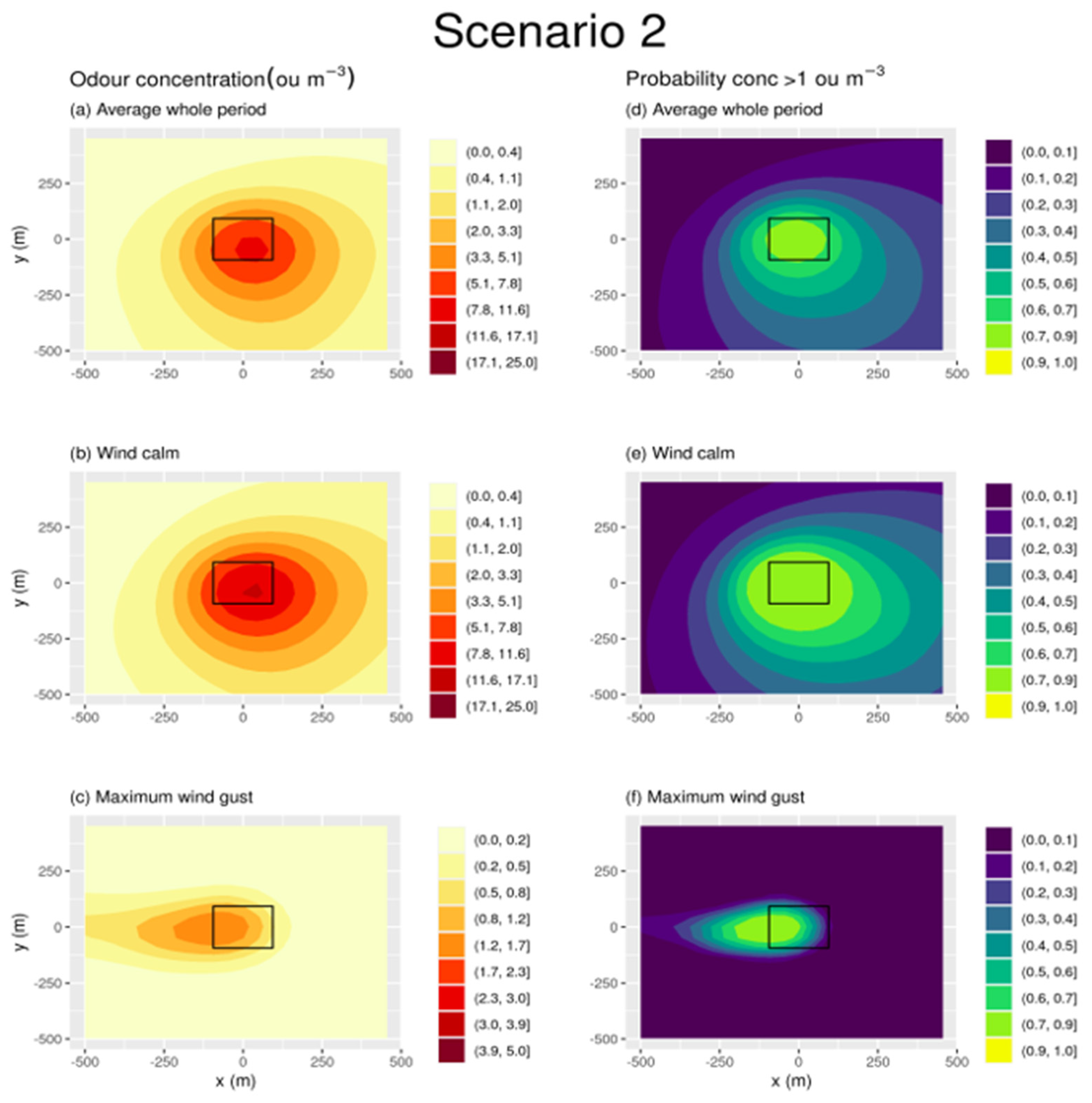
| Scenario 2 | ||||||
| Min. | 0.05 | 0.06 | 0 | 0.02 | 0.02 | 0 |
| 1st Qu. | 0.33 | 0.44 | 1.93 × 10⁻⁵ | 0.11 | 0.17 | 0 |
| Median | 0.83 | 1.13 | 2.5 × 10⁻³ | 0.24 | 0.34 | 0 |
| Mean | 1.46 | 2.01 | 0.17 | 0.26 | 0.36 | 0.06 |
| 3rd Qu. | 1.76 | 2.38 | 0.12 | 0.37 | 0.5 | 3 × 10⁻⁷ |
| Max. | 8.55 | 12.03 | 1.66 | 0.81 | 0.88 | 0.84 |
| Scenario 2bis0 | Scenario 2bis | |||
|---|---|---|---|---|
| Concentration [ou m−3] | Exceedance Probability [-] | Concentration [ou m−3] | Exceedance Probability [-] | |
| Min. | 0 | 0 | 2.3 × 10⁻⁴ | 0 |
| 1st Qu. | 2.99 × 10⁻⁵ | 0 | 0.01 | 0 |
| Median | 7.1 × 10⁻³ | 0 | 0.09 | 0 |
| Mean | 0.13 | 0.03 | 0.15 | 6.79 × 10⁻⁹ |
| 3rd Qu. | 0.18 | 4.9 × 10⁻⁵ | 0.28 | 0 |
| Max. | 1.20 | 0.67 | 0.50 | 1.26 × 10⁻⁶ |
Disclaimer/Publisher’s Note: The statements, opinions and data contained in all publications are solely those of the individual author(s) and contributor(s) and not of MDPI and/or the editor(s). MDPI and/or the editor(s) disclaim responsibility for any injury to people or property resulting from any ideas, methods, instructions or products referred to in the content. |
© 2023 by the authors. Licensee MDPI, Basel, Switzerland. This article is an open access article distributed under the terms and conditions of the Creative Commons Attribution (CC BY) license (https://creativecommons.org/licenses/by/4.0/).
Share and Cite
Vuolo, M.R.; Acutis, M.; Tyagi, B.; Boccasile, G.; Perego, A.; Pelissetti, S. Odour Emissions and Dispersion from Digestate Spreading. Atmosphere 2023, 14, 619. https://doi.org/10.3390/atmos14040619
Vuolo MR, Acutis M, Tyagi B, Boccasile G, Perego A, Pelissetti S. Odour Emissions and Dispersion from Digestate Spreading. Atmosphere. 2023; 14(4):619. https://doi.org/10.3390/atmos14040619
Chicago/Turabian StyleVuolo, Maria Raffaella, Marco Acutis, Bhishma Tyagi, Gabriele Boccasile, Alessia Perego, and Simone Pelissetti. 2023. "Odour Emissions and Dispersion from Digestate Spreading" Atmosphere 14, no. 4: 619. https://doi.org/10.3390/atmos14040619