Article

Effects of Microphysics Parameterizations on Forecasting a Severe Hailstorm of 30 April 2021 in Eastern China

1
Key Laboratory of Geographic Information Science, Ministry of Education, East China Normal University, Shanghai 200241, China
2
School of Geographic Sciences, East China Normal University, Shanghai 200241, China
3
East China Air Traffic Management Bureau, CAAC, Shanghai 200335, China
4
Climate, Environment and Sustainability Center, School of Atmospheric Science, Nanjing University of Information Science and Technology, Nanjing 210044, China
5
Shanghai Central Meteorological Observatory, Shanghai 200030, China
*
Author to whom correspondence should be addressed.
Atmosphere 2023, 14(3), 526; https://doi.org/10.3390/atmos14030526
Submission received: 3 February 2023 / Revised: 28 February 2023 / Accepted: 7 March 2023 / Published: 9 March 2023
(This article belongs to the Special Issue Improving Extreme Precipitation Simulation)

Abstract

:
On the evening of 30 April 2021, a severe hailstorm swept across eastern China, causing catastrophic gale and damaging hailstones. This hailstorm event was directly caused by two mesoscale convective systems associated with strong squall lines, with mid-level cold advection from the northeast cold vortex, and strong low-level convergence associated with the low-level vortex and wind shear line. Double nesting of the high-resolution weather research and forecasting model (9–1 km) is utilized to simulate this hailstorm with five microphysics schemes. The radar-based maximum estimated size of hail (MESH) algorithm, differential reflectivity and fractions skill scores were used to quantitatively evaluate the precision. All schemes basically captured the two squall lines that swept through eastern China, although they appeared one or two hours earlier than observation. Particularly, Goddard and Thompson performed better in the MESH swath and fractions skill scores among the five different schemes. However, Thompson most realistically captured the reflectivity pattern, intensity and vertical structure of mesoscale convective systems. Its high-reflectivity column corresponded to the maximum center of the hail mixing ratio within the updraft region, which is consistent with the characteristics of a pulse-type hailstorm in its mature phase.

1. Introduction

Hailstorm is a major type of severe weather frequently occurring in China [1]. It is mainly associated with relatively short-lived mesoscale convective systems (MCSs) and accompanied by severe hail and intense winds, causing great damage to agriculture and construction. Although the hailstorms show a higher frequency in western China [2], they generally produce a larger size of hailstones in eastern China [3,4], which is more vulnerable to the destruction of hailstorms due to its dense population and developed economy. For instance, the hailstorm that occurred in eastern China during the evening of 30 April 2021 caused hailfalls in 9 cities and 20 counties in Jiangsu province, with the maximum size of hailstones reaching 1–3 cm, and a gale of 45.4 m/s in Nantong city. Subsequently, it greatly affected the southeast of Shanghai city with the strongest orange hail warning issued since 2017. The orange hail warning means hail may happen within six hours. According to the 2021 China Climate Bulletin, the gale accompanied with severe hailstorm resulted in 17 deaths in total and 11,000 hectares of agricultural damages with a direct economic loss of 160 million in Chinese Yuan. Thus, this severe hailstorm process is worthy of an in-depth study, and the accurate forecast of hail is particularly crucial for weather disaster prevention. All the related toponomy can be found in Figure 1.
However, it is still a great challenge to accurately predict the hailstorm and the associated pattern, and the phase of precipitation, especially the hail. Difficulties mainly arise from the inadequate understanding of the dynamics and microphysical processes of hailstorms and the improper model physics representations. For the first aspect, the direct observation of hailstorms or hailstones is still deficit, hindering the complete understanding of hailstorm evolution processes. Currently, radar observation is being used as the most effective tool for severe weather monitoring and nowcasting, and different algorithms have been developed to quantitatively predict hail. For instance, based on basic reflectivity and wet bulb temperature height at 0 °C and −20 °C levels, Witt et al. (1998) proposed a hail detection algorithm to calculate the severe hail index (SHI) and the maximum estimated size of hail (MESH) [5]. With the development of dual-polarization radar observation, differential reflectivity has become a good indicator to distinguish hailstones from intense rainfall. It depends on the ratio of the horizonal and vertical axes of precipitation particles, with large values for raindrops but near 0 for hail particles [6,7]. Jung et al. (2008, 2010) built a dual-polarization radar simulator to calculate the differential reflectivity, which is very useful for verifying the hail intensity and location [8,9]. For example, this simulator has been used in the study of Sun and Dai (2019) to evaluate the forecast of hail that occurred in southern Jiangsu Province and Shanghai City during the night of 28 April 2015 [10]. Moreover, the type of hydrometeors can be further classified by using the dual-polarization radar derived variables [11]; for example, the large and small hailstones could be distinguished [12]. In recent years, the number of dual-polarization radars in China has increased and more radar observations can be used to improve hail forecast [13]. Thus, Shanghai Nanhui dual-polarization radar variables are utilized in this case to verify the model simulation of hailfalls.
Regarding the hail forecasting, a high-resolution numerical weather prediction model (NWP) with detailed microphysics representations of hail processes is specifically required. Because the hailstorm itself is a small-scale and fast developing system, and the production and growth of hailstones are very complex during the hailstorm evolution, previous studies have attempted to use convective-permitting models (CPMs) with grid spacings below 4 km to make an ideal experiment or real forecast of hailstorms [14], but there is no consensus on the proper choice for grid spacing to explicitly represent convection and the hailstorm simulations (Wang et al., 2021) [15]. For instance, Luo et al. (2017) and Luo et al. (2018) compared the simulation results of two hailstorm processes in Zhejiang and Jiangsu provinces with grid spacings of 3 km and 1 km, respectively, and found that the results of two different model resolutions were similar [16,17]. As such, they pointed out that a model resolution of 3 km can provide qualitatively valid simulation of a hailstorm, although the grid spacing of 3 km is too large compared to the hailstorm scale. However, Bryan and Morrison (2012) performed sensitivity experiments in an ideal simulation of a squall line process, and suggested that the most realistic results can be achieved when the model resolution was increased to 0.25 km [18]. Given that the grid spacings at 1 km are generally adequate for explicitly resolving strong convection in current weather or climate modeling studies (Liang et al., 2019) [19], this study uses the Weather Research and Forecasting Model (WRF) with double nesting of a large grid ratio (9:1 km) to perform the hailstorm forecast.
More attention has been paid to the impacts of different microphysics parameterization schemes on hail forecast. The WRF model mainly incorporates the bulk schemes with different complexity, from the simplest one-moment schemes only predicting the mixing ratio for each hydrometeor, to the improved two-moment and multi-moment schemes which typically add the prediction of number concentration and reflectivity factor [20]. The prediction of additional moments allows greater flexibility in representing the particle size distributions and hence affects microphysics processes, such as the sedimentation (treatment of size sorting) and the rain evaporation rates. There has been a trend toward the use of more complex microphysics schemes; however, the effects of different schemes are highly case dependent, and it is still controversial about how to choose the proper scheme. For instance, Milbrandt and Yau (2006) showed that two- and three-moment schemes of Milbrandt–Yau (MY) produced a better prediction of hailstorm and the surface precipitation than a one-moment scheme [21]; Luo et al. (2017) performed an explicit prediction of hailstorm in Zhejiang province, China, by using the three-moment scheme of MY, and it produced a better forecast of the size and amount of hail at the surface than the one-moment scheme [16]. Yin et al. (2019) compared the impacts of four microphysics schemes in the WRF model on the simulation of a hailstorm process in Jiangsu province. Their results suggested the Morrison two-moment scheme produced the best forecast, but the MY two-moment (MY2) scheme did not agree well with the observations [22]. Thus, this study selects five widely used microphysics schemes with different complexity (number of species and moment, or ice processes) to examine their effects on high-resolution forecast of hailstorm.
The objective of this study is to investigate the 1-km WRF simulation of this severe hailstorm of 30 April 2021 in eastern China using five different microphysics schemes, with the focus on the model differences in the spatial distribution and vertical structure of radar composite reflectivity associated with the dominant MCSs, the distribution of MESH and differential reflectivity, as well as the fractions skill score (FSS) for hailfalls. The simulated environmental indices, microphysical characteristics and dynamic structures of this hailstorm are further analyzed to explore the possible causes for the model sensitivity.
The following paper is organized as follows. Section 2 examines the synoptic environment and primary impacting systems for the occurrence of this hailstorm event, with the focus on the evolution characteristics of MCSs based on satellite and radar observation. Section 3 describes the WRF model experiments with five different microphysics schemes and model evaluation metrics. The simulations from five sensitivity experiments are compared in Section 4 against radar-derived composite reflectivity, MESH, differential reflectivity, and FSS for hailfalls. The possible physical understanding of these model differences is described in Section 5. Section 6 summarizes the main conclusions and discussions.

2. Case Overview

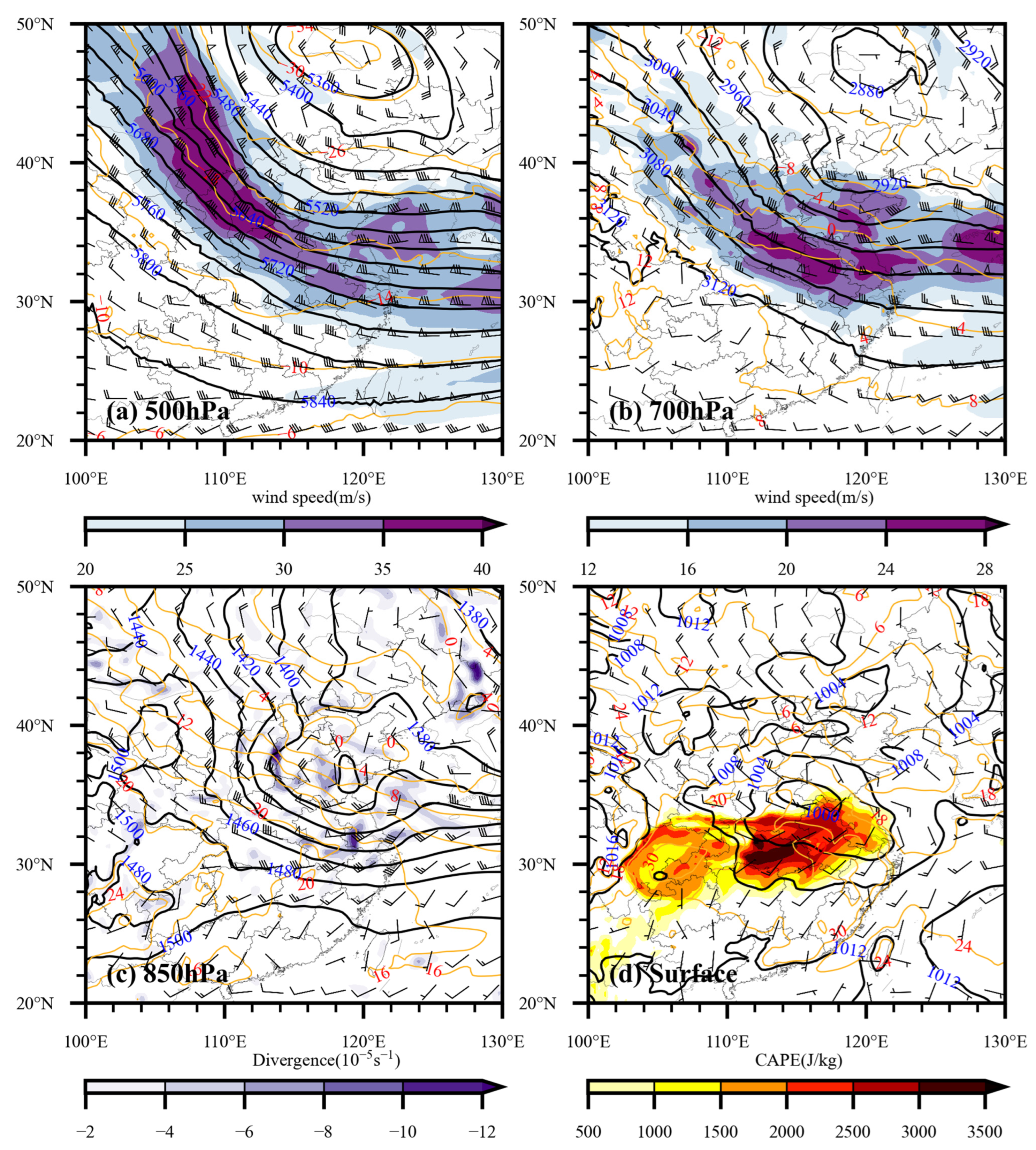
2.1. Synoptic Environment

Figure 2 presents the synoptic-scale environment in the early stage of this hailstorm process at 0600 UTC (Coordinated Universal Time) on 30 April 2021, based on the fifth generation of ECMWF (European Centre for Medium-Range Weather Forecasts) reanalysis data (ERA5) with a resolution of 0.25° × 0.25° [23]. On that afternoon, at 500 hPa, a deep cold vortex system was located in northeast China, and eastern China was controlled by a northwesterly wind and the associated cold air advection from the back of the cold vertex in the upper levels. The jet streak was located in the central and northern part of China, with the maximum wind speed over 40 m/s. Jiangsu province and Shanghai city were located to the north of the jet-exit region where the upper-level divergence predominates (Figure 2a). At 700 hPa, a short-wave trough in the bottom of the northeast cold vortex was moving eastward and the northwesterly wind largely affected the eastern China (Figure 2b). At 850 hPa, a low pressure existed in the north of Jiangsu province with large-scale convergence in its southern region. The north–south temperature gradient in Jiangsu province exceeded 8 °C, and warm and strong southwesterly winds prevailed over the south of Jiangsu province (Figure 2c). The mid-level cold air advection from the northeast cold vortex superimposed on the low-level warm advection from the south, resulting in high convective available potential energy (CAPE) exceeding 1000 J/kg shown at the surface, where the convection is initiated by the convergence forcing associated with the wind shear line in the southeast of the low surface pressure (Figure 2d).
Figure 3 presents the sounding data from the University of Wyoming at three stations to analyze the environment conditions for the hailstorm initiation, including Sheyang and Nanjing stations in Jiangsu province and Baoshan station in Shanghai City shown in Figure 1b. At 0000 UTC—approximately 8 h before convection was initiated in the north of East China—three stations were already under the combined influence of the cold and dry air in the middle to upper levels, and low-level warm air advection with vertically clockwise rotation of horizontal winds below 850 hPa, but the convective instability and the water vapor condition were not yet sufficient (Figure 3a,c,e). After 12 h at 1200 UTC, the main body of the squall line had passed Sheyang station, and the entire vertical layer from the lower to upper troposphere was close to saturation (Figure 3b). At this time, in the sounding of Baoshan and Nanjing stations, there both existed strong convective instability with high CAPE values of 441.9 and 2035.4 J/kg. The vertical wind shear between 0–6 km reached 34.1 and 35.8 m/s, respectively. The presence of high CAPE and strong vertical wind shear, together with the low-level convergence forcing associated with low surface pressure and wind shear line, is conductive to the initiation of severe storms and favors the development of intense MCSs. Moreover, a deep layer of cold, dry air above 700 hPa above a low-level warm, moist layer near the ground is especially favorable for larger hailstones because moister air could reduce the melting of hailstones, as suggested by the previous studies of Craven et al. (2004) and Luo et al. (2017) [17,24]. More convective environmental indices are calculated in Section 5, and the calculation methods are given in Appendix A.

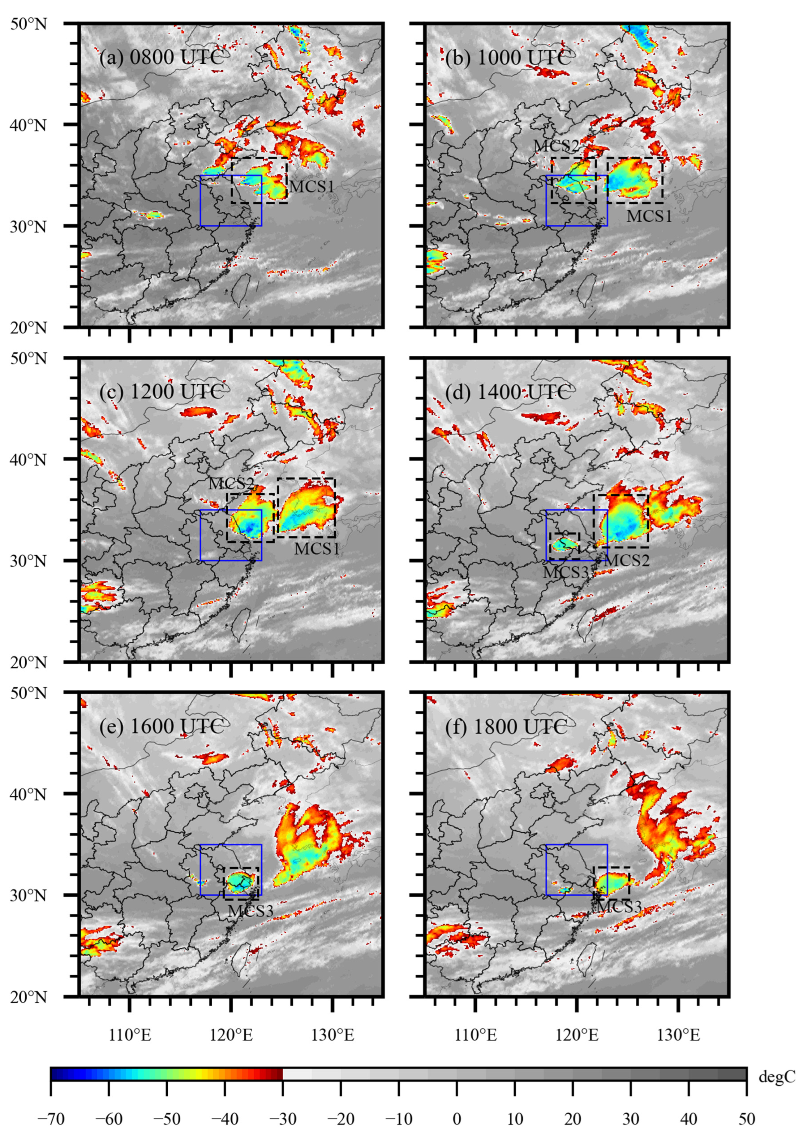
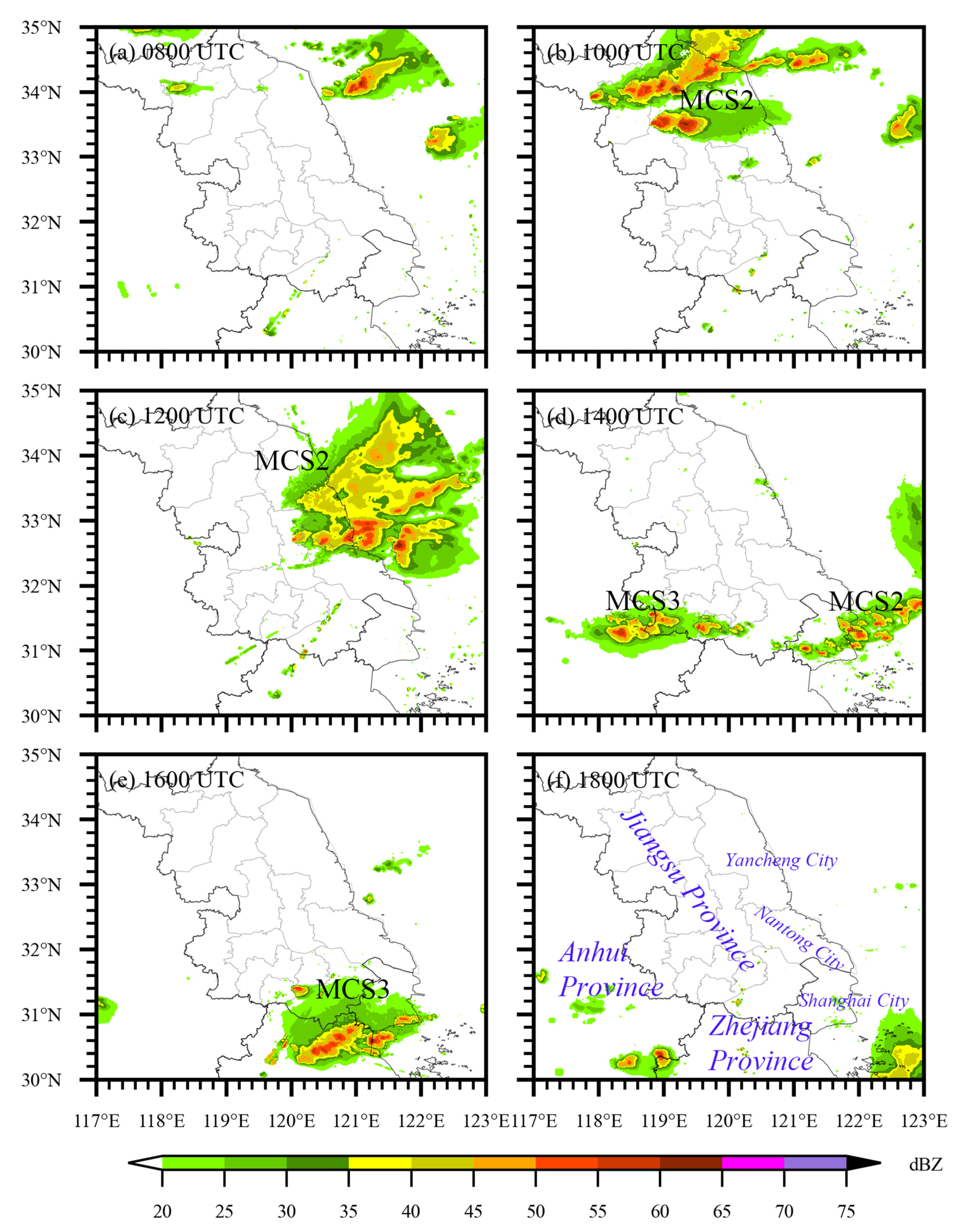
2.2. Mesoscale Convective Systems Observed by Satellite and Radar

Here, a MCS is defined as a cluster of low IR temperature (below −32 °C) with a major axis of 100 km or more. Figure 4 demonstrates the evolution of MCSs associated with this hailstorm event from 0800 UTC to 1800 UTC by using the TBB (Black Body Temperature) in 10.8-μm infrared band derived from the AGRI (Advanced Geostationary Radiation Imager) of the FY-4A (Feng-Yun 4A) geostationary satellite. The sub-satellite point was at 104.7° E and the geometric correction was done. The parallax effect was not considered. However, the position offset can be neglected according to radar imagery (Figure 5). At 0800 UTC, MCS1 had already formed over the East China Sea, with a TBB below −55 °C (Figure 4a). However, MCS1 did not directly affect eastern China. At 1000 UTC, MCS1 and MCS2 are developing rapidly. MCS2 with TBB lower than −55 °C in the northern region of Jiangsu province was rapidly strengthening as it moved southeast (Figure 4b). About two hours later, this intensified MCS2 began to affect the coastal areas of Jiangsu province at 1200 UTC, with the lowest TBB value reaching −60 °C (Figure 4c), causing severe hailfalls and disastrous winds. Subsequently, MCS2 continued to move eastward and affected Shanghai about four hours later at 1400 UTC with its low TBB tail (Figure 4d); at the same time, a new MCS3 generated at 1300 UTC and then intensified to affect the border of Anhui and Jiangsu province at 1400 UTC, with the lowest TBB about −50 °C (Figure 4d). At 1600 UTC, MCS2 moved eastward into the sea, rapidly weakened. MCS3 maintained its intensity (Figure 4e). MCS3 weakened and moved eastward into the sea at 1800 UTC, with only a few isolated convective cells left on land (Figure 4f).
Figure 5 presents the composite reflectivity fields from nine operational radars in Jiangsu province and Shanghai city during 0800 to 1800 UTC at 2-h intervals. The processing of radar data in this section and the following use python’s pyart library [25]. The Nanhui radar is the Weather Surveillance Radar 88 Doppler (WSR-88D), which is a dual-polarization radar with S-band. The others are the China New Generation Weather Radar (CINRAD), which are S-band, single-polarization radars. Some of the CINRAD radars have been upgraded, but the radar base data has no dual-polarization variables, which means they are still considered as single-polarization radars. The squall line associated with MCS2 was initially formed at the bottom of the upper-level cold vortex (Figure 5a), and strengthened rapidly as it moved to the southeast. It began to affect the north of Jiangsu province at 1000 UTC, with a maximum reflectivity of 65 dBZ (Figure 5b). At 1200 UTC, the squall line moved to the east of Jiangsu province, and mainly affected Yancheng and Nantong city in Jiangsu province (Figure 5c). It continued to move southeastward and affected Shanghai after two hours at 1400 UTC, and a new squall line associated with MCS3 was generated in the east of Anhui province and subsequently affected the southwest of Jiangsu province (Figure 5d). At 1600 UTC, the squall line affecting Shanghai moved eastward into the sea, while the squall line affecting Anhui and Jiangsu moved to the north of Zhejiang (Figure 5e). Both of them quickly decayed after two hours at 1800 UTC (Figure 5f).
To sum up, this hailstorm affecting Jiangsu province and Shanghai city was directly caused by MCS2 and MCS3 associated with strong squall lines. The synoptic-scale environment for the development of MCS2 and MCS3 is characterized by high CAPE, strong vertical wind shear, and the presence of mid-level cold air advection from the northeast cold vortex superimposed on a low-level warm, moist layer near the ground, as well as low-level convergence forcing associated with surface low pressure and wind shear line.

3. Model Experiments and Evaluation Methods

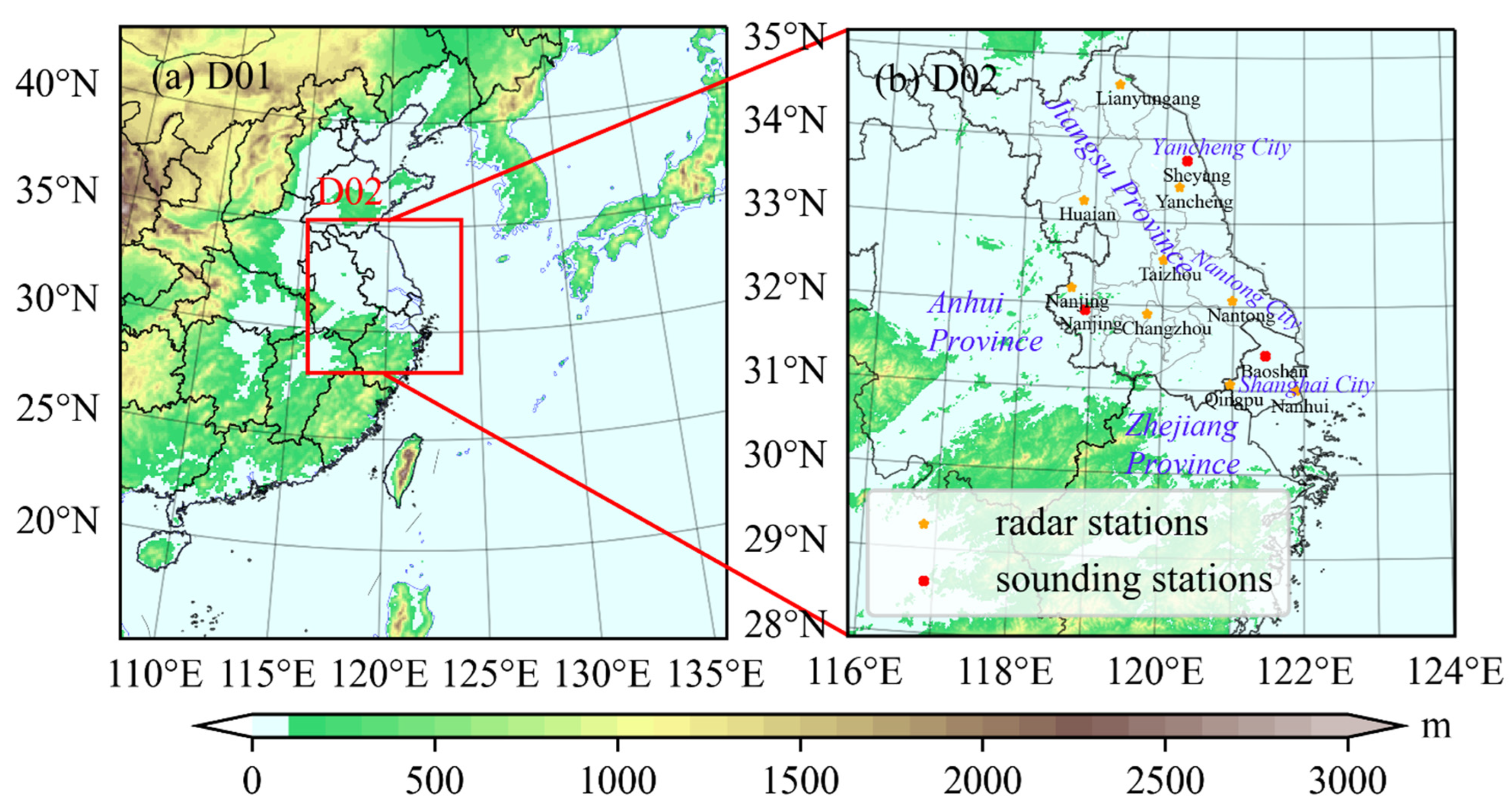
3.1. Model Configuration and Experimental Design

This hailstorm case is simulated by using the WRF version 3.9.1.1 (Skamarock et al., 2008) [20]. As shown in Figure 1a, double-nesting domains are constructed with the outer domain centered at 30° N, 122° E, and the Lambert conformal map projection is used. The outer domain (D01) is made up of 802 × 802 grid points and the inner domain (D02) is made up of 401 × 401 grid points, with horizontal grid spacing of 9 km and 1 km, respectively. Two domains use one-way nesting without feedback and the same vertical discretization of 51 levels. The 30-arc-second USGS terrain data and 21-category, 2-m resolution MODIS land use/cover data are adopted for static surface conditions.
All simulations were initialized at 0000 UTC on the 30 April 2021 and run for 18 h, with 6 h used for spin-up. The integral time steps are 54 s for both D01 and D02. The top pressure is 50 hPa. 1° × 1° NCEP-FNL Operational Global Analysis data were used as initial conditions and boundary conditions, with a 6-h interval. Cumulus parameterization was turned on at D01 using the traditional Kain and Fritsch scheme [26], and off at D02. Surface layer parameterization was the revised MM5 scheme [27]. Land surface was the Unified Noah Land Surface model [28]. Planetary boundary layer parameterization was tested, and Shin-Hong Scale-aware scheme [29] was used in this study.
Five convection-permitting experiments using different microphysics parameterization schemes are conducted to examine the sensitivity of hail forecast, including WRF Single-moment 6-class (WSM6) [30], Goddard [31,32], Thompson [33], Milbrandt–Yau two-moment (MY2) [34,35] and Morrison two-moment (Morrison2) [36]. These five schemes are different in their prediction moments and the types of ice particles, such as small ice, snow, graupel or hail. Among them, the WSM6 scheme predicts the mixing ratio only for six species, including cloud water vapor, cloud water, cloud ice, rain, snow and graupel, while Goddard 3ICE and Morrison2 scheme are both two-moment schemes that additionally predict the number concentration for the same six species. Differently, the Thompson scheme is between single and double moment because this scheme predicts the number concentration for cloud ice and cloud rain (Zhu et al., 2022) [37], and the MY2 scheme is the only one that explicitly predicts hail in the ice processes. We added hail_opt = 1 for WSM6 and Morrison2 and gsfcgce_hail = 1 for Goddard in the namelist.input file, which means hail was included in graupel in the WRF outputs.

3.2. Maximum Estimated Size of Hail

As hail reports and station observations are insufficient, the radar-based maximum estimated size of hail (MESH) algorithm was adopted to quantitatively evaluate the maximum expected hail size. This algorithm was developed by Witt et al. (1998) and improved by Murillo and Homeyer (2019, 2021) [5,38]. Three parameters are particularly needed in the algorithm, including the basic reflectivity, the height of 0 °C, and −20 °C wet bulb temperature. The calculation formula are as follows:
First, the hail kinetic energy ( E ˙ ) is calculated:
E ˙ = 5 × 10 6 × 10 0.084 Z W ( Z )
where Z is the basic reflectivity, with units in dBZ. The weight W ( Z ) means the transition zone between rain and hail, which is calculated by Formula (2):
W ( Z ) = { 0                           Z Z L Z Z L Z U Z L       Z L < Z < Z U 1                             Z Z U
where Z L and Z U are set to 40 and 50 dBZ, respectively. Then, the temperature-based weight is calculated:
W T ( H ) = { 0                               H H 0 H H 0 H m 20 H 0         H 0 < H < H m 20     1                         H H m 20
where H is the height above radar level. H 0 and H m 20 are the heights of 0 °C and −20 °C wet bulb temperature, respectively. Here, the observed 0 °C and −20 °C heights are obtained from the ERA5 data.
All outputs above are used to calculate severe hail index (SHI):
SHI = 0.1 H 0 H T W T ( H ) E ˙ d H
The origin formula of MESH derived from SHI is:
MESH = 2.54 ( SHI ) 0.5
Based on more hail cases, this formula was updated by Murillo and Homeyer (2019, 2021) as:
MESH = 15.096 ( SHI ) 0.206
For model evaluation, the observed radar reflectivity datasets and model simulated reflectivity outputs are both interpolated to the 1-km model grid to derive MESH.

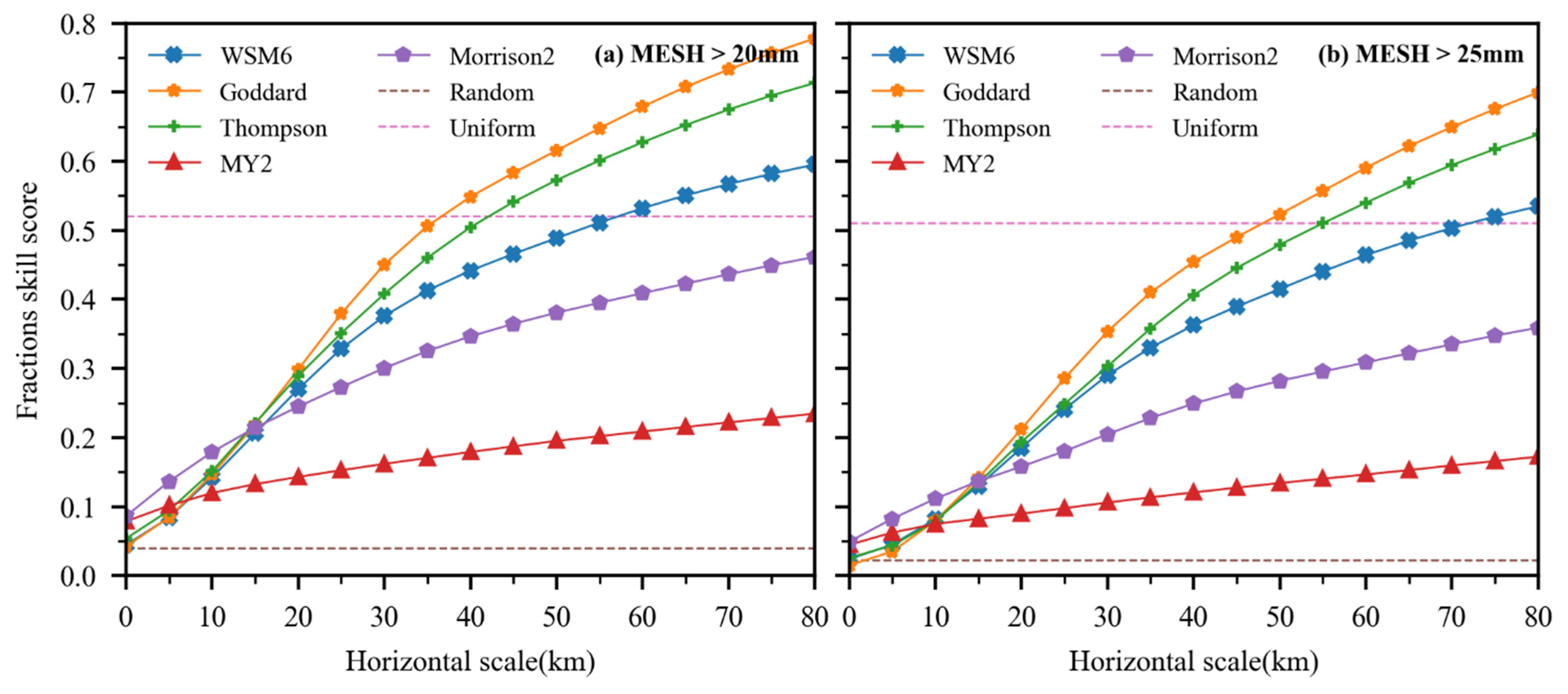
3.3. Fractions Skill Scores for Hail Prediction

Fractions skill score (FSS) was proposed by Roberts and Lean (2008) to better evaluate the convective weather forecast, compared to the traditional threat score [39]. It is a kind of fuzzy verification method, which considers a certain space and time uncertainty by comparing the characteristics of the adjacent area of the corresponding point in prediction and observation fields. FSS has become a popular spatial verification method for high-resolution models (Tang et al., 2018) [40]. The FSS equations for evaluating the hail prediction are as follows:
FSS ( n ) = 1 M S E ( n ) M S E ( n ) r e f
where n is the length of neighborhood, M S E ( n ) is the mean squared error considering the adjacent area, and M S E ( n ) r e f is the largest possible MSE calculated between forecast and observation. More accurately, we need two metrics:
FSS random = f o
FSS uniform = 0.5 + f o / 2
where f o is the number of precipitation (here it is the hail) grids divided by the number of total grids. FSS random is the score of random prediction, which is equal to f o numerically. For small-scale and low-probability events, f o is close to 0, and FSS uniform is close to 0.5, which is relatively low. For large-scale and high-probability events, f o is close to 1, and FSS uniform is close to 1, indicating a high predictive skill. When the FSS ( n ) exceeds FSS uniform , it means that the predictive skill is improved by expanding the grid scale to include more valuable prediction information.

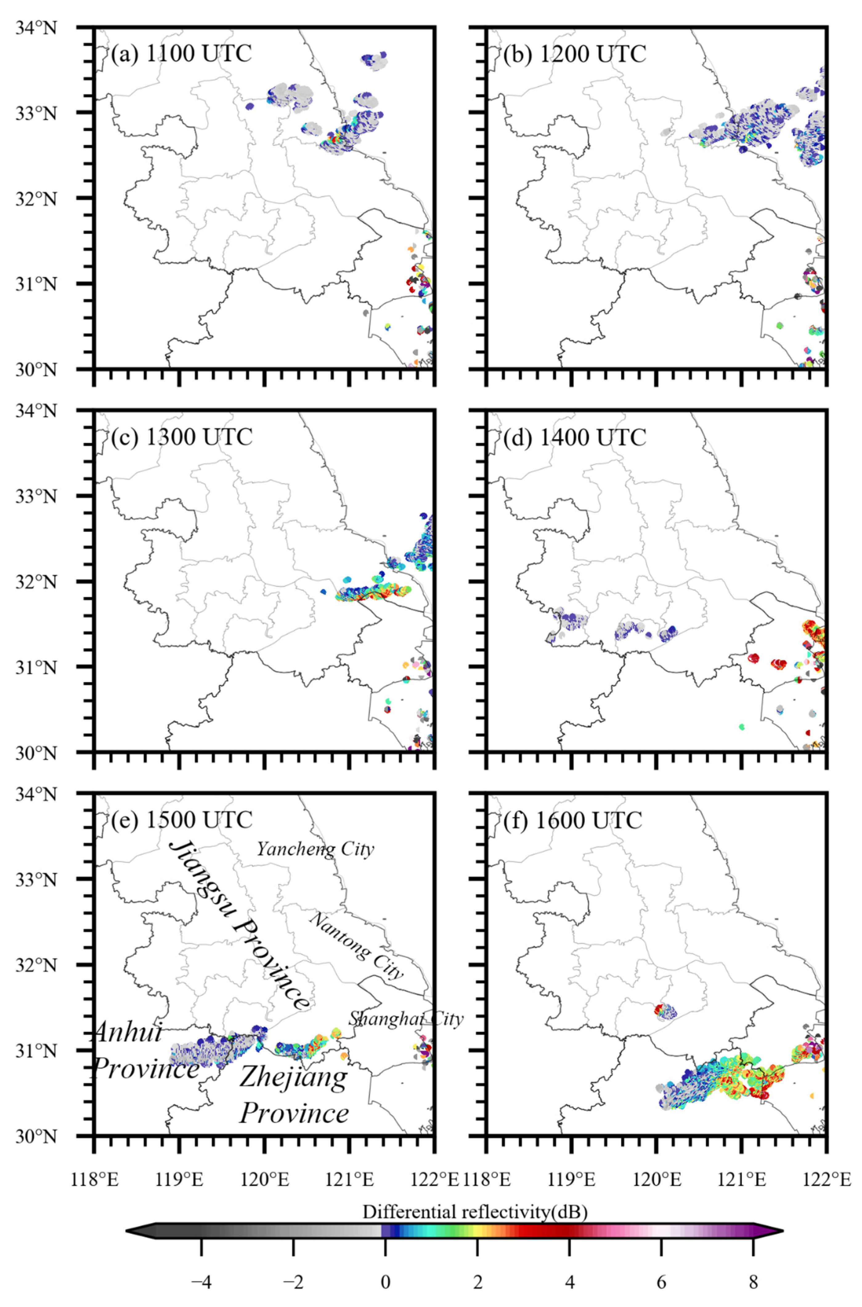
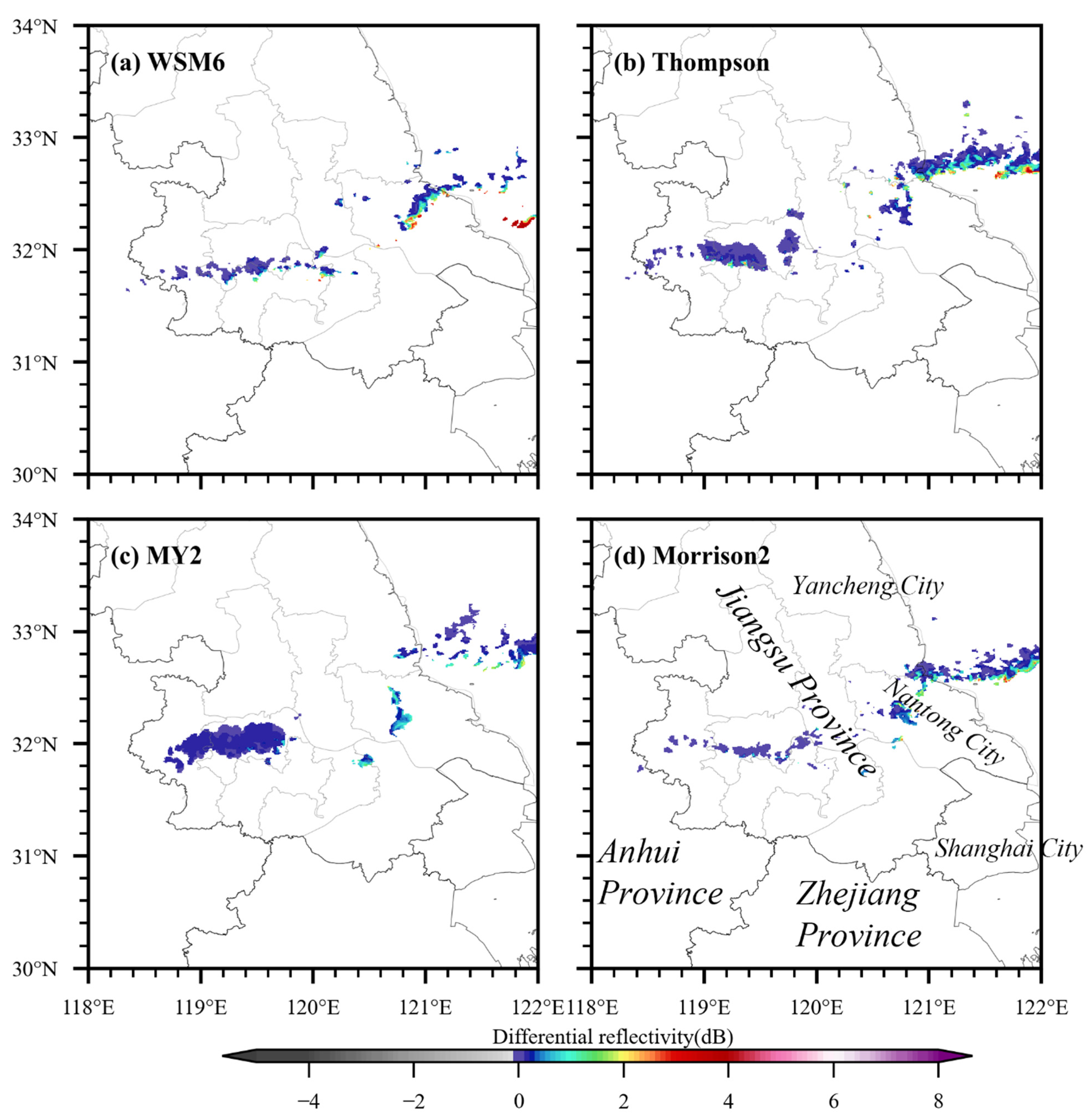
3.4. Differential Reflectivity

Differential reflectivity is a useful variable that dual-polarized radar can provide to determine the shape of particles. Specifically, a large raindrop is elliptical and differential reflectivity is large, but hail is nearly spherical, and its differential reflectivity is small and less than 2.0 dB (Sun and Dai, 2019) [10]. As such, the hail falling region is characterized by high values of basic reflectivity and low values of differential reflectivity. In this study, Shanghai Nanhui WSR-88D dual-polarization radar was available to provide more particle size information in addition to the basic reflectivity, and the observations at a 0.5° elevation angle were used because the dual-polarization radar variables are more significant at lower elevations.
For model simulations, CAPS-PRS_V1.1 (CAPS Polarimetric Radar data Simulator) [8,9] is used to extract the WRF outputs to calculate dual-polarization variables, which can be interpolated to Nanhui station at a 0.5° elevation angle. This was developed by the Center for Analysis and Prediction of Storms at the University of Oklahoma and is currently applicable to five microphysical schemes in the WRF model. More details about the calculations of differential reflectivity can be referred to Jung et al. (2010) [9].

3.5. Severe Convection Environmental Indices

The occurrence of severe convective weather requires specific environmental conditions, including convective available potential energy, atmospheric instability, vertical wind shear, the height of melting and freezing level, etc. These conditions are defined by a variety of environmental indices listed in Table 1, which can be calculated based on the sounding data of stations near the occurrence of convection.
Convective available potential energy (CAPE) measures the potential energy that is available for convection. Convective inhibition energy (CIN) represents the amount of work the environment must do on the parcel to raise the parcel to its level of free convection. K index considers both the lapse rate and moisture conditions in the middle and lower troposphere, and a larger K index means a higher instability. Total totals index (TT) includes both the 850-hPa dewpoint and the static stability between 850 hPa and 500 hPa, measuring the instability and moisture conditions of the middle and lower troposphere. Lifted index (LI) measures the difference of temperature between the environment and a lifted parcel, with negative values representing the potential instability. Severe weather threat index (SWEAT) considers both kinetic and thermodynamic in a single index, which is used mainly for analyzing the potential for severe thunderstorm with the values of about 300 and higher. Wind shear between 0–6 km (WS_6) is the variation of mean horizontal wind with height, strongly affecting the maintenance of severe thunderstorm. In addition, 0 °C wet bulb temperature height (WBT_0) and −20 °C wet bulb temperature height (WBT_N20) are important indicators for the growth of hailstones.
The study of these environmental indices helps to understand the physical process of the convection initiation and development, which can be good indicators for severe weather forecast. More details about the indices can be found at https://www.weather.gov/lmk/indices (accessed on 3 February 2023) by the National Weather Service. The formulas for calculating the indices are listed in the Appendix A.

4. Simulation Results and Evaluation

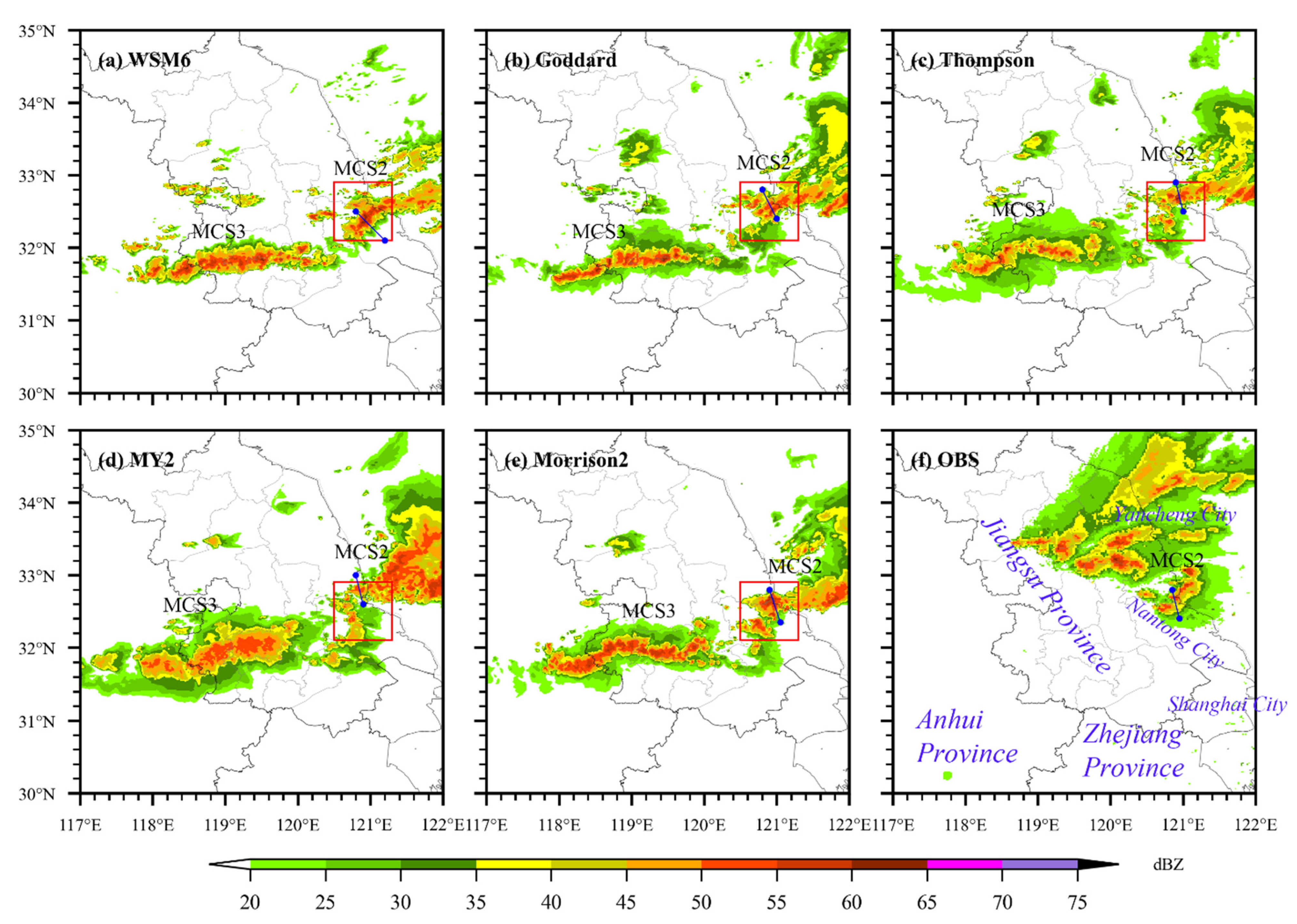
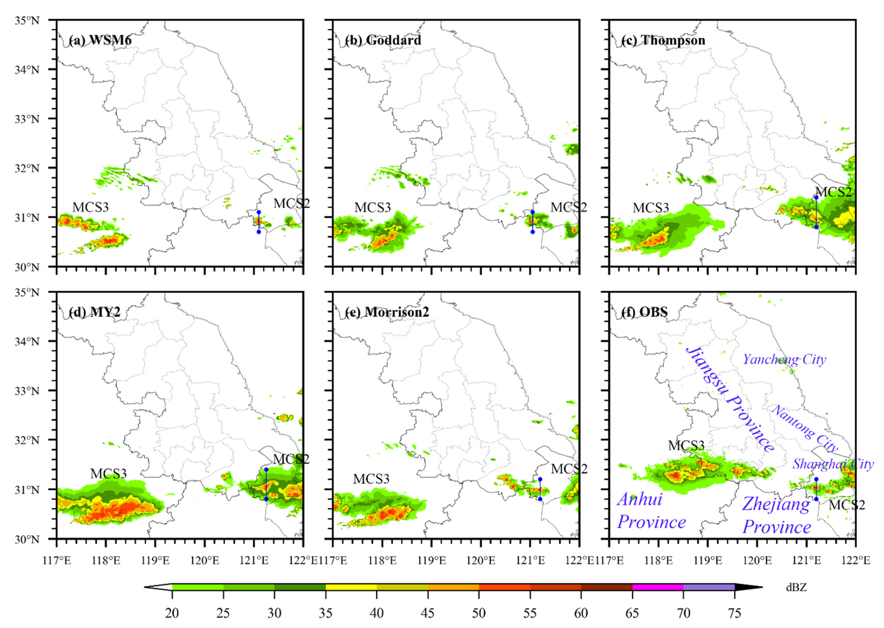
4.1. Comparison of Model Simulated Composite Reflectivity

The following radar reflectivity and cross-section interpolation were calculated by python’s package wrf-python [41]. Figure 6 compares the composite reflectivity fields simulated by WRF using five different microphysics schemes against radar observations at 1100 UTC when the simulated MCS2 reached its peak intensity and started to affect the east of Jiangsu province. All simulations basically captured the strong MCS2, along with the squall line that swept through the eastern Jiangsu, although it appeared one hour earlier than observation. In addition, the most pronounced difference between the simulation and observation is that the MCS3 and the associated newly generated squall line (the western part in Figure 6) at the border between Jiangsu and Anhui province appeared at 1100 UTC in the simulation, which was two hours earlier than the observation. This early initiation of convection could be caused by the impact of the convective parameterization scheme in the outer domain (Liang et al., 2019) [19], or the inherent problem of convection-permitting simulation in the inner domain with too frequent occurrence of convection (Zhu et al., 2018) [42].
Given that severe hail and gale occurred at 1100 UTC in Nantong city, Jiangsu province, the simulation at this time presents close to the best match with the observation, and thus this study first focuses on the hailstorm induced by MCS2 affecting Nantong (red box in Figure 6). The vertical cross sections of simulated reflectivity through the maximum reflectivity core (the locations are shifted slightly) are also compared in Figure 7. In observation, the strong squall line affecting the eastern Jiangsu province showed a linear array of convection systems with high-reflectivity areas reaching 55–60 dBZ, and a wide precipitating area around 20–35 dBZ. In the vertical structure, the high-reflectivity column (>55 dBZ) was located at 1–3 km below the 0 °C level, with the near-ground reflectivity exceeding 50 dBZ (Figure 7f). This corresponds to previous studies of Heymsfield (1983) [43] and Luo et al. (2017) [16], in which they both found that the hail collection rate of rain below the melting level is larger, and the maximum hailstone growth rate occurs before falling to the ground.
Table 2 lists the results which may reflect the strong convection structure of different schemes and observation, including maximum reflectivity, height of maximum reflectivity core, echo top (over 20 dBZ) and maximum reflectivity near surface (below 1 km). Compared to the observation, except for MY2, all schemes overestimated the maximum reflectivity. The height of the maximum reflectivity core was overestimated and echo top was underestimated by all schemes at 1100 UTC.
The model simulations of the reflectivity pattern and vertical structure are categorized into three groups: (1) the WSM6 and Goddard schemes overestimated the intensity of high-reflectivity region, of which the reflectivity can reach 60–65 dBZ (Figure 7a,b). In addition, the former produced a smaller coverage area of precipitation (20–35 dBZ, Figure 6a), but a stronger intensity of reflectivity near the ground (Figure 7a). (2) The MY2 scheme underestimated the intensity of reflectivity (Figure 6d). The maximum reflectivity core extended up above the −20 °C level, which is much higher than the observation. The maximum reflectivity near the surface is too low compared to other schemes (Figure 7d). (3) The Thompson and Morrison schemes better captured the maximum intensity of the high-reflectivity region (55–60 dBZ, Figure 7c,e). However, Thompson had a lower height of maximum reflectivity core, close to the 0 °C level, which is more consistent with observations.
Figure 8 presents the simulated composite reflectivity fields at 1400 UTC when the MCS2 and its associated squall line moved eastward and affected Shanghai with its low TBB tail. All simulations captured the storm cell at the tail of the MCS2, but the simulated MCS3 was still located in Anhui province, which was westward compared to the observation. Figure 9 also plots the vertical cross sections of reflectivity fields through the maximum reflectivity core of this storm cell in western Shanghai at this time. In the observation, the storm weakened compared to that at 1100 UTC. It showed a reduced intensity of the high-reflectivity column with the maximum value around 55–60 dBZ, and the cloud top height was about 11 km.
The model simulations of the reflectivity pattern and vertical structure were also concluded: (1) The WSM6 scheme was able to capture the maximum reflectivity core (55–60 dBZ), compared to other schemes. However, it overestimated the intensity of reflectivity near the ground (Figure 9a). (2) The Goddard, Thompson, MY2 and Morrison2 schemes underestimated the maximum reflectivity. Goddard performed the worst among them because its maximum reflectivity core was too high, at over 8 km (Figure 9b). Thompson performed better in echo top and maximum reflectivity near the ground. Its high-reflectivity column (50–55 dBZ) between 3–8 km was consistent with observations (Figure 9c).
To sum up, Thompson is the best scheme compared to the other schemes since it was able to capture the reflectivity pattern and vertical structures at 1100 UTC and 1400 UTC.

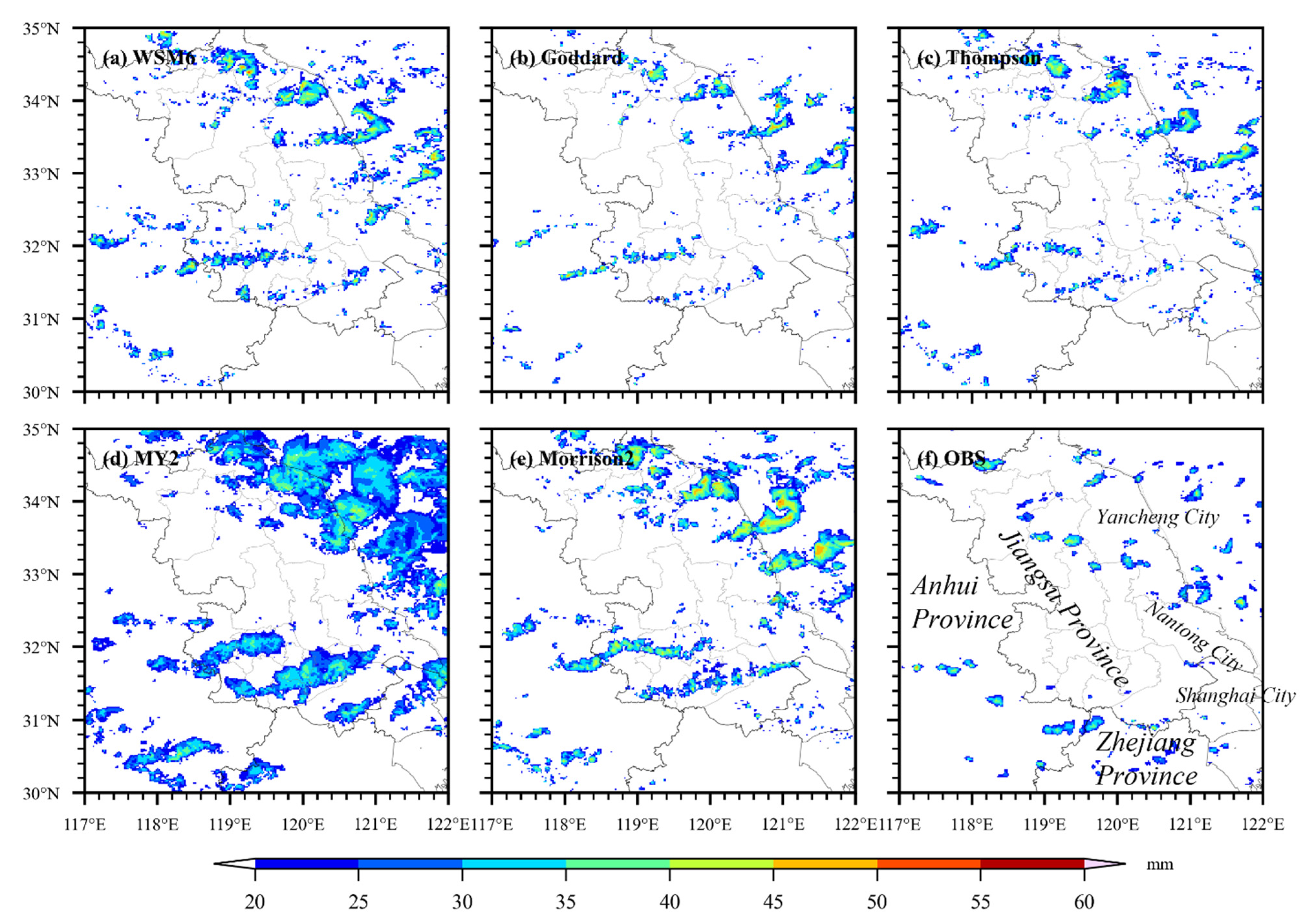
4.2. Comparison of Model Simulated MESH and FSS Scores

Swaths of MESH simulated by WRF using five different microphysics schemes between 0600 UTC and 1800 UTC at a 1-h interval are compared against radar-derived values in Figure 10. In the observation, there were two hail bands, one moving from the northwest to the southeast of Jiangsu province, and the other moving from Anhui province to the south of Jiangsu province. They corresponded well to the MCS2 and MCS3 previously analyzed. Most radar-derived MESH was below 35 mm, but could reach 40 mm in some areas (Figure 10f). All schemes were able to capture the paths of two MCSs, but the positions were a little farther north than the observation. The model differences of MESH can be also categorized into three groups accordingly: (1) the WSM6 and Morrison2 schemes both produced larger areas of MESH over 20 mm, but the maximum value of MESH associated with MCS2 in the Morrison2 scheme exceeded 45 mm, which was larger than that in the WSM6 scheme; (2) the coverage of MESH over 20 mm by the MY2 scheme was too large and unreal, but the values of MESH were generally less than 40 mm; (3) the Goddard and Thompson schemes showed relatively good results, except that the hail falling areas of MESH over 20 mm were more scattered and slightly larger than the observation.
Figure 11 demonstrates the FSS scores for model-simulated hail at varying horizonal grid scales for MESH over 20 mm and 25 mm, respectively. The results showed that each scheme had better results for smaller hailstones (MESH > 20 mm). Even if the horizontal scale increased to 80 km, the prediction accuracy still could not be improved in the MY2 and Morrison2 schemes. Their FSS scores were basically less than 0.5, primarily due to their overestimated coverage area of MESH. The Goddard and Thompson schemes showed significantly improved predictive skills with the increasing horizontal scale. For MESH over 20 mm, the Goddard scheme was better than the original prediction when the horizontal scale reached 40 km, compared to 45 km for Thompson and 60 km for WSM6 (Figure 11a). For MESH over 25 mm, the predictive skills were degraded. When the horizontal scale was increased to 50, 55 and 75 km, respectively, Goddard, Thompson and WSM6 schemes started to provide useful predictions (Figure 11b). That indicates that five schemes tend to have higher predictive skills for smaller hails, among which the Goddard and Thompson schemes showed significant advantages over others in MESH prediction with consistently higher FSS scores.

4.3. Comparison of Model Simulated Differential Reflectivity

Figure 12 presents the differential reflectivity fields derived from Shanghai Nanhui dual-polarization radar observations at a 0.5° elevation angle during 1100 UTC to 1600 UTC when the cross-correlation coefficient was greater than 0.8 and basic reflectivity was over 40 dBZ. The 0.5° elevation angle was selected because we concern hailfalls at the low level and near the ground. Basic reflectivity below 40 dBZ was excluded in order to examine the large particles. A correlation coefficient below 0.8 was excluded to eliminate some clutters, although some clutters still existed near the radar. At 1100–1200 UTC, differential reflectivity was close to 0 in the coastal area of Jiangsu, indicating that the hailstorm was affecting Yancheng and Nantong city from the north to the south with large hailfalls. At 1300 UTC, the tail associated with MCS2 began to affect Shanghai, and subsequently produced hail in the north of Shanghai. At 1400 UTC, small melting hailstones were detected in the west of Shanghai, due to the occurrence of high differential reflectivity. At the same time, the new squall line associated with MCS3 also brought hails in the southwest of Jiangsu province, and during 1500–1600 UTC, the new squall line on the west side affected the junction of provinces, producing large hailstones.
Figure 13 compares the model simulated differential reflectivity fields at 1100 UTC from different microphysics schemes. Here, the result from the Goddard scheme was not included because CAPS-PRS_v1.1, which we used to derive the differential reflectivity, does not support the WRF simulation from the Goddard scheme currently. The comparison shows that, at 1100 UTC, the four schemes were all able to capture the large hail falling area over Nantong city in the east of Jiangsu province produced by MCS2, while the simulated hail in the west of Jiangsu province produced by MCS3 was generally two hours earlier than the observation, which is consistent with the previous findings. Among the simulations, the Thompson scheme can better capture the large hail area in the east of Jiangsu province, while the other schemes generally underestimated the coverage area, especially the WSM6 and MY2 schemes. For large hail over the west of Jiangsu province induced by MCS3, the falling area of the MY2 scheme was too large, while that of the WSM6 and Morrison2 schemes were small and more scattered. Therefore, in comparison with the radar-derived differential reflectivity, the Thompson scheme showed advantages over other schemes in the simulation of large hail falling areas in Jiangsu province.

5. Discussion

In the following section, possible causes for the model sensitivity will be analyzed from the effects of different microphysics schemes, with respect to the vertical distributions of cloud hydrometeors, dynamic structures and convective environmental indices associated with the hailstorm.

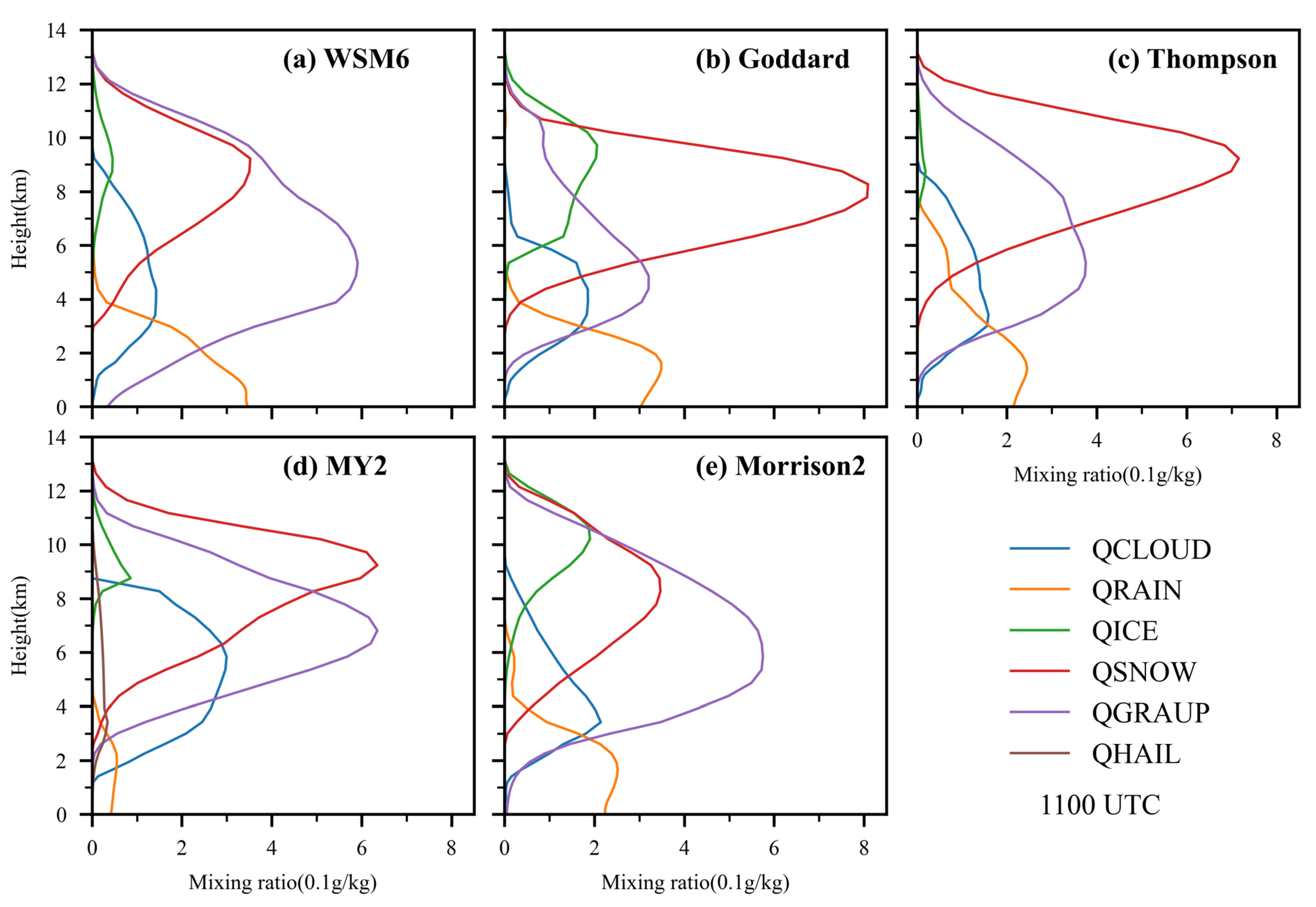
5.1. Vertical Distributions of Cloud Hydrometeors’ Mixing Ratio

Figure 14 compares the simulated vertical distributions of mixing the ratio of cloud water (QCLOUD), rain (QRAIN), ice (QICE), snow (QSNOW) and graupel (QGRAUP) averaged over the hailstorm region induced by MCS2 at 1100 UTC. It should be noted that hail (QHAIL) is distinguished from graupel only in the MY2 scheme; hail is included in graupel in the other schemes. Corresponding to the simulated vertical structure of composite reflectivity, model differences in cloud hydrometeors’ distribution can be also categorized into three groups: (1) both the WSM6 and Morrison2 schemes produced more graupel than snow; graupel was especially formed near the ground up to 12 km, with the peak value appearing at the height of 5 km, which contributed to the strong intensity of the high-reflectivity column. The difference is that the WSM6 scheme produced more cloud rain near the ground than the Morrison2 scheme, resulting in its higher reflectivity near the ground shown in Figure 7a. (2) The MY2 scheme produced a comparably higher value of graupel and snow above 6 km, but much less graupel, snow and rain near the ground. This contributed to the high-reflectivity region located at a higher level above the −20 °C level (around 6 km) and the weaker reflectivity near the ground for the MY2 scheme. However, cloud water in the MY2 scheme was larger than that in the other schemes, with the peak appearing at around 6 km. In particular, hail was co-located with cloud water. This was supported by the finding of Luo et al. (2017) [16], in which the hail collection of cloud water was shown as an important hailstone growth process in the MY2 scheme and the maximum collection rate occurred around 6 km. (3) The Goddard and Thompson schemes produced similar vertical distributions of cloud hydrometeors, with more snow at higher levels around 8 km and less graupel at lower levels around 4 km. The latter primarily contributed to the lower position and intensity of the high-reflectivity column simulated by this group than that of the first group. However, the difference between these two schemes is that the Goddard scheme produced much more cloud ice above 6 km, corresponding to its overestimated intensity of the high-reflectivity column (>55 dBZ) extending up above −20 °C level (~6 km) in Figure 7b.
Therefore, the simulated characteristics of composite reflectivity are closely related to the distribution of cloud hydrometeors, which is greatly affected by the assumptions of ice-phased particles and associated microphysical processes in different schemes. First, the possible reasons why the first group (WSM6 and Morrison2 scheme) both produced a higher QGRAUP and a lower QSNOW, but the Morrison scheme produced a lower QRAIN near the ground are: (1) both schemes adopt the spherical and constant density assumption for snow particles. Compared to the assumption of non-spherical and varying density of snow particles, it is more likely to produce larger snow particles with stronger riming or deposition growth, leading to more graupel. (2) Both schemes include additional growth processes of graupel by collecting the cloud ice or snow and from the water vapor autoconversion (Hong et al., 2006; Morrison et al., 2009) [30,36]. (3) The Morrison2 scheme particularly increased the rain evaporation rate in the convective region at the mid-levels, resulting in reduced convective updrafts and less rain falling on the ground. Second, the relatively higher QGRAUP above 6 km simulated by the MY2 scheme is ascribed by the inclusion of moderate density graupel formed from heavily rimed ice or snow (Luo et al., 2017) [16,36]. Third, the reasons why the third group (Goddard and Thompson scheme) generally produced higher QSNOW and lower QGRAUP but too little QICE in the Thompson scheme are: (1) the dry collection of ice/snow by graupel in the Goddard 3ICE-graupel scheme is eliminated to reduce the unrealistic presence of graupel in the cloud anvil, but it resulted in larger cloud snow content (Tao et al., 2016) [32]; (2) the ice particles with radii greater than 200 μm are all converted to snow particles in the Thompson scheme, leading to more snow, less graupel, but too little cloud ice.

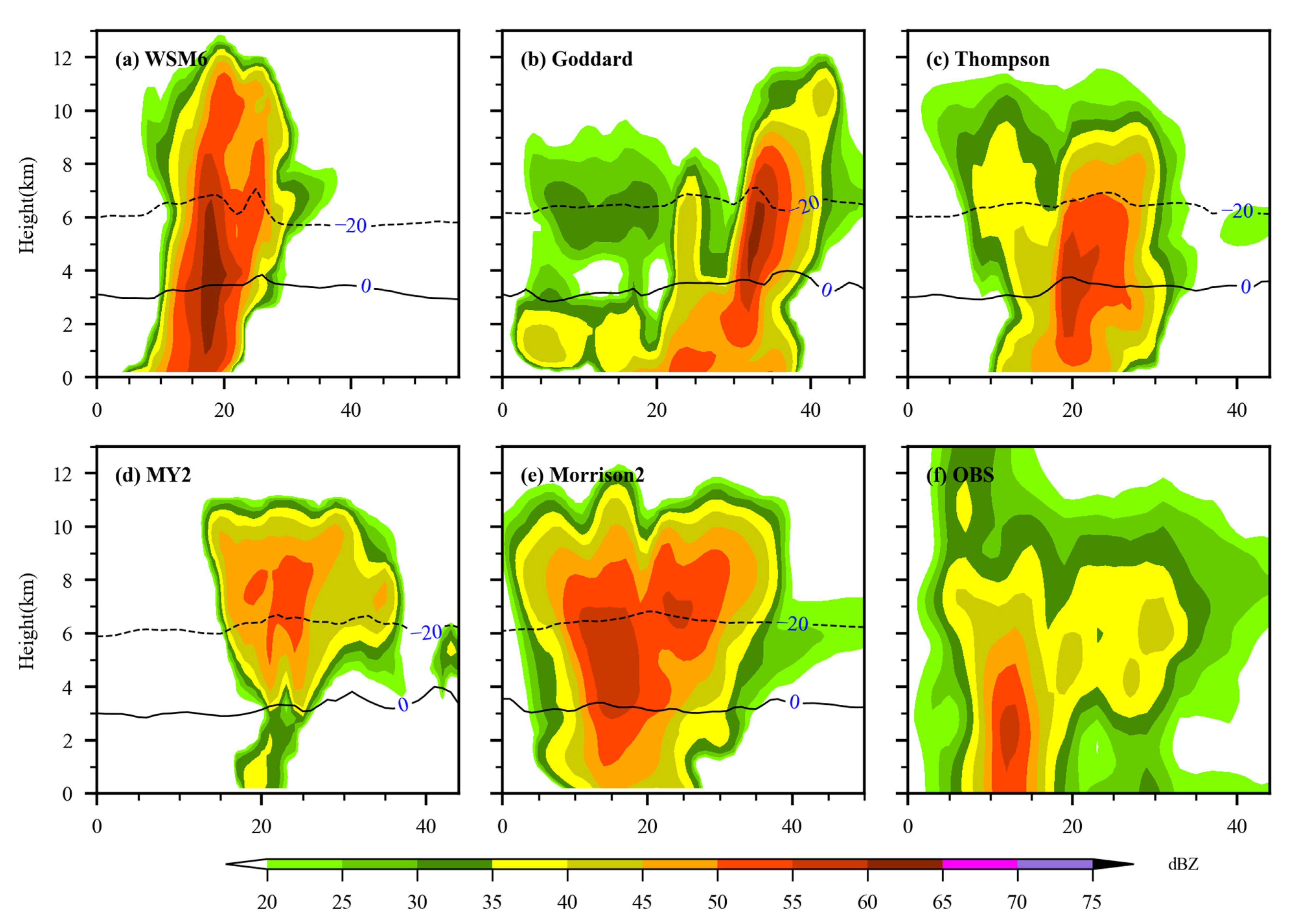
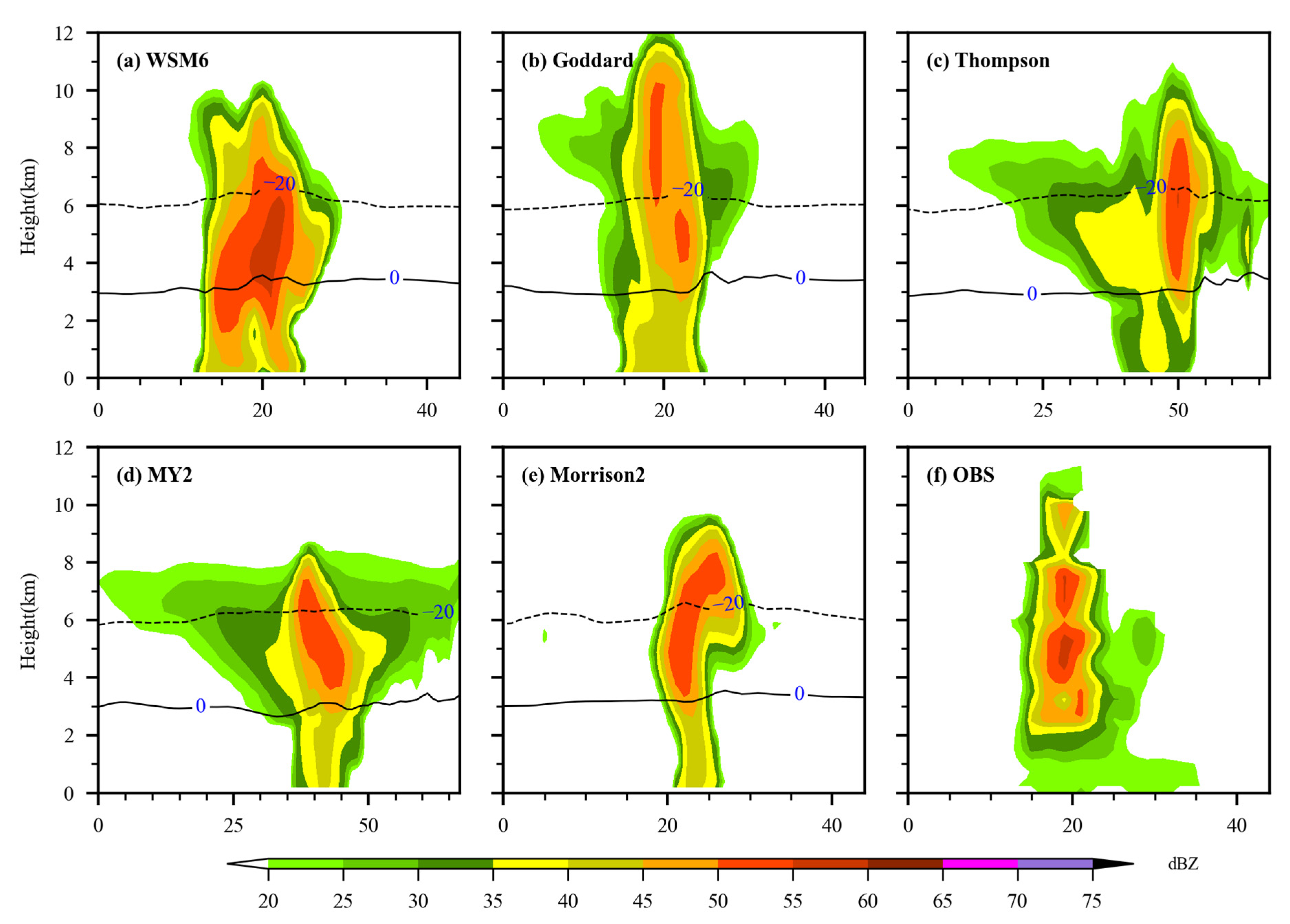
5.2. Dynamical Structures of Hailstorm

The dynamic structure of hailstorm and the associated microphysical characteristics are also quite sensitive to the choice of microphysics schemes. Figure 15 examines the vertical cross section of updrafts and downdrafts and the hail/graupel mixing ratio in five simulations at 1100 UTC along the lines of Figure 6. We consider the sum of the graupel and hail mixing ratio in the MY2 scheme since MY2 distinguished hail from graupel. Combined with the vertical distribution of composite reflectivity in Figure 7, the simulated dynamical structures of hailstorms can be also categorized into three groups: (1) in the WSM6 and Morrsion2 schemes, the high-reflectivity column corresponded to the maximum center of the hail mixing ratio, which was located in the downdrafts from the rear side of updrafts. Specifically, the WSM6 scheme simulated the strongest updraft, exceeding 28 m/s, but the corresponding hail mixing ratio was lower, around 4 g/kg, while the strong downdrafts in the rear side were below the 0 °C level, corresponding to the maximum hail mixing ratio of up to 8 g/kg between the 0 °C and −20 °C level. The Morrison2 scheme produced stronger downdrafts and a higher hail mixing ratio than the WSM6 scheme. This dynamical feature of both schemes well explained their overestimated intensity of the high-reflectivity column from the near ground extending up to 8 km, as well as the larger value of MESH. (2) In the MY2 scheme, the high-reflectivity column with lower intensity corresponded to the center of the hail mixing ratio around 4 g/kg, which was located within the updraft region but at a higher position above the −20 °C level. The weak downdrafts below the updraft region indicates that the hail flux near ground was small, explaining the lower intensity of near-ground reflectivity and the smaller value of MESH. (3) In the Goddard and Thompson schemes, the high-reflectivity column corresponded to the maximum center of the hail mixing ratio, which was located within the updrafts region. This feature was consistent with the characteristics of the pulse-type hailstorm at its mature phase, suggested by Luo et al. (2017) [16]. Among them, the Thompson scheme produced stronger downdrafts below the 0 °C level with large hail flux extending to the ground, and also more realistically captured the size-sorting features of hailfalls, with high reflectivity intensity increasing as the height reduced.

5.3. Convective Environmental Indices

Table 3 further compares the simulated convective environmental indices in Baoshan station at 1200 UTC when the observed sounding data from the University of Wyoming were available. Model simulations well captured K, TT, WBT_0 and WBT_20. Since these indicators reflect the temperature and humidity of the environment, the overall simulations of thermodynamic condition are believable. Among all the schemes, Thompson performed best in K and TT, although its WBT_20 was relatively lower.
If the absolute value is considered, all schemes overestimated CAPE, CIN and LI. These indices involve the lifting of the air parcel. Since the environmental condition is relatively well simulated, the systematic bias of these indices may be related to the starting conditions of the air parcel. Local differences at the surface can lead to very different results.
WS_6 was underestimated by all schemes. This shows that the simulations of wind speed are not as accurate as environment conditions such as temperature. The systematic bias may be related to the choice of planetary boundary layer scheme or other physical schemes. The hailstorms were accompanied by gale, so the simulation of strong winds is also important. MY2 produced the strongest WS_6. In addition, it also produced the maximum CAPE, the minimum CIN and the lowest WBT_N20. These indices are conductive to the development of both severe convection and hailfalls. This may explain why the MY2 scheme overestimated the coverage area of MESH over 20 mm (Figure 10d).
There are significant differences in the simulation of the SWEAT index. This may be due to the fact that the SWEAT index is a complex index, taking into account both kinetic and thermodynamic conditions. Goddard and Thompson schemes performed better in the SWEAT index, which may be related to their good performance on MESH.
More improvements need to be made from other physical parameterizations that affect the convection initiation, and development, such as deep convection and boundary layer processes.

6. Conclusions

This paper focuses on the severe hailstorm that swept across eastern China on the evening of 30 April 2021, causing gale and damaging hailstones of 1–3 cm in diameter in Nantong city and multiple reports of severe hailfalls in Shanghai city. The high-resolution weather research and forecasting model with double nesting using a large grid ratio (9 km–1 km) is utilized to simulate this hailstorm, with the focus on the effects of five widely used microphysics schemes, including WSM6, Goddard, Thompson, MY2 and Morrison2 schemes. The radar-based maximum estimated size of hail (MESH) algorithm, fractions skill scores (FSS) and differential reflectivity from dual-polarization radar observation in Shanghai Nanhui station are used to quantitively evaluate the hail predictions. The simulated microphysical characteristics, dynamic structures and environmental indices of this hailstorm are further analyzed to explore the possible causes for the model sensitivity. The main results are concluded as follows:
(1) This hailstorm affecting Jiangsu province and Shanghai city was directly caused by two mesoscale convective systems (MCSs) associated with strong squall lines. The synoptic-scale environment for the development of these MCSs is characterized by high CAPE, strong vertical wind shear, and the presence of mid-level cold air advection from the Northeast cold vortex superimposed on a low-level warm, moist layer near ground, as well as low-level convergence forcing associated with surface low pressure and wind shear line.
(2) All schemes captured the strong MCS2 along with the squall line swept through the eastern Jiangsu, although it appeared one hour earlier than observation. The simulated MCS3 associated with a newly generated squall line at the border between Jiangsu and Anhui province appeared at 1100 UTC, which was two hours earlier than the observation.
(3) The Thompson scheme best captured the reflectivity pattern and vertical structure of MCS2 compared to the other four schemes. Its high-reflectivity column (50–55 dBZ) between 3–8 km was consistent with observations. It also performed better in the maximum reflectivity, height of maximum reflectivity core, echo top and maximum reflectivity below 1 km at 1100 UTC and 1400 UTC.
(4) The Goddard and Thompson schemes best captured MESH and MESH swaths caused by MCS2 and MCS3, which was consistent with observations. They have the first and second highest FSS score. WSM6, MY2 and Morrison2 performed worse because they produced larger coverage of MESH or larger MESH.
(5) The simulated characteristics of composite reflectivity are closely related to the distribution of cloud hydrometeors, which is greatly affected by the assumptions of ice-phased particles and associated microphysical processes in different schemes. For instance, the Goddard and Thompson schemes produced more snow than graupel, with snow at level around 8 km and graupel at level around 4 km. This could be due to two reasons. One is because the Goddard scheme eliminates the dry collection of ice/snow by graupel to reduce the unrealistic presence of graupel in the cloud anvil, but it results in larger cloud snow content; the other is because the Thompson scheme converts the ice particles with radii greater than 200 μm to snow particles, which results in more snow, less graupel, but too little cloud ice. The distribution of cloud hydrometeors is consistent with the high-reflectivity column in the Thompson scheme, and the Thompson scheme produced stronger downdrafts below the 0 °C level with large hail flux extending to the ground, and more realistically captured the size-sorting features of hailfalls, with high reflectivity intensity increasing as the height reduced.
(6) All simulations well captured four convective environmental indices, including K, TT, WBT_0 and WBT_N20. However, the systematic bias existed in CAPE, CIN, LI and WS_6, which may be caused by the starting conditions of the air parcel and other physical schemes. Thompson performed better in K, TT, WBT_0 and SWEAT.
To sum up, Thompson is the best scheme in simulating hail compared with other schemes. The shortcoming of this paper is that we only studied the influence of hail in this process, but the process also produced gale. Other physical options need to be tested because of the systematic biases of environmental indices discussed. Complex microphysics schemes may improve the physical realism, but they may not necessarily produce consistently better results due to other model deficiencies or inconsistency with other physical parameterizations. Given that more advanced multi-moment microphysics schemes have been developed to explicitly predict the hail, such as the Milbrandt and Yau three-moment scheme [34,35], further study is required to examine its performance in simulating more hailstorm cases over eastern China.

Author Contributions

Conceptualization, F.J. and F.Q.; methodology, F.J.; software, R.W. and Q.L.; validation, F.J.; formal analysis, F.J.; investigation, B.C. and C.W.; resources, B.C. and C.W.; data curation, R.W. and Q.L.; writing—original draft preparation, F.J.; writing—review and editing, F.Q.; visualization, F.J.; supervision, F.Q.; project administration, F.Q.; funding acquisition, F.Q. All authors have read and agreed to the published version of the manuscript.

Funding

This study was funded by the Shanghai 2021 “Scientific and technological innovation action plan” Natural Science Foundation (Grant No. 21ZR1420400), and the National Natural Science Foundation for Young Scientist of China (Grant No. 41605079).

Institutional Review Board Statement

Not applicable.

Informed Consent Statement

Not applicable.

Data Availability Statement

ERA5 on pressure levels can be download at: https://cds.climate.copernicus.eu/cdsapp#!/dataset/reanalysis-era5-pressure-levels?tab=overview (accessed on 3 February 2023). ERA5-land can be downloaded at: https://cds.climate.copernicus.eu/cdsapp#!/dataset/reanalysis-era5-land?tab=overview (accessed on 3 February 2023). NCEP-FNL can be downloaded at: https://rda.ucar.edu/datasets/ds083.2/#!access (accessed on 3 February 2023). FY-4A TBB can be downloaded at: http://satellite.nsmc.org.cn/PortalSite/Data/Satellite.aspx?currentculture=en-US (accessed on 3 February 2023). Radiosonde sounding data can be downloaded at: http://weather.uwyo.edu/upperair/bufrraob.shtml (accessed on 3 February 2023). CAPS-PRS_v1.1 can be downloaded at: https://arps.caps.ou.edu/downloadpyDualPol.html (accessed on 3 February 2023).

Acknowledgments

The model simulation ERA5 reanalysis dataset was downloaded from https://cds.climate.copernicus.eu/ (accessed on 3 February 2023). We acknowledge the High Performance Computing Center of Nanjing University of Information Science & Technology and the ECNU Multifunctional Platform for Innovation 001 facilities for their support of this work.

Conflicts of Interest

The authors declare no conflict of interest.

Appendix A

Some environment indices mentioned in Table 1 were calculated by the following formulas (according to Metpy) [44]:
C A P E = R d L F C E L ( T parcel T env ) d l n ( p )
C I N = R d S F C L F C ( T parcel T env ) d l n ( p )
where R d is the gas constant, E L is the equilibrium level, L F C is the level of free convection, S F C is the start level, p is the pressure, T parcel is the parcel temperature and T env is the environment temperature.
K and TT were calculated as follows:
K = ( T 850 T 500 ) + T d 850 ( T 700 T d 700 )
TT = ( T 850 + T d 850 ) 2 T 500
where T is the temperature, T d is the dewpoint temperature, and the lower right-hand number means the pressure level.
LI was calculated as follows:
LI = T 500 T parcel _ surface _ 500
where T parcel _ surface _ 500 is the temperature of the lifted parcel from the surface.
SWEAT was calculated as follows:
SWEAT = 12 T d 850 + 20 ( TT 49 ) + 2 f 850 + f 500 + 125 ( S + 0.2 )
where f is the wind speed in knots. Shear term S is equal to sin ( d d 850 d d 500 ) , where d d is the wind direction. S is set to zero when 130 d d 850 250 , 210 d d 500 310 , d d 500 d d 850 > 0 or both wind speeds are greater than or equal to 15 knots.
WS_6 was calculated as follows:
WS _ 6 = V 6 V 0
where V 6 is the wind vector at 6 km height, V 0 is the wind vector at surface.
Other complex indices calculations also followed Metpy. They can be found on https://unidata.github.io/MetPy/dev/api/generated/metpy.calc.html (accessed on 3 February 2023).

References

  1. Zhang, Q.H.; Ni, X.; Zhang, F.Q. Decreasing trend in severe weather occurrence over China during the past 50 years. Sci. Rep. 2017, 7, 43210. [Google Scholar] [CrossRef] [PubMed] [Green Version]
  2. Zhang, C.X.; Zhang, Q.H.; Wang, Y.Q. Climatology of Hail in China: 1961–2005. J. Appl. Meteorol. Climatol. 2008, 47, 795–804. [Google Scholar] [CrossRef]
  3. Li, X.F.; Zhang, Q.H.; Zou, T.; Lin, J.P.; Kong, H.; Ren, Z.H. Climatology of Hail Frequency and Size in China, 1980–2015. J. Appl. Meteorol. Climatol. 2018, 57, 875–887. [Google Scholar] [CrossRef]
  4. Ni, X.; Muehlbauer, A.; Allen, J.T.; Zhang, Q.; Fan, J. A Climatology and Extreme Value Analysis of Large Hail in China. Mon. Weather Rev. 2020, 148, 1431–1447. [Google Scholar] [CrossRef]
  5. Witt, A.; Eilts, M.D.; Stumpf, G.J.; Johnson, J.T.; Mitchell, E.D.; Thomas, K.W. An enhanced hail detection algorithm for the WSR-88D. Weather Forecast. 1998, 13, 286–303. [Google Scholar] [CrossRef]
  6. Bringi, V.N.; Seliga, T.A.; Aydin, K. Hail detection with a differential reflectivity radar. Science 1984, 225, 1145–1147. [Google Scholar] [CrossRef]
  7. Herzegh, P.H.; Jameson, A.R. Observing precipitation through dual-polarization radar measurements. Bull. Am. Meteorol. Soc. 1992, 73, 1365–1374. [Google Scholar] [CrossRef]
  8. Jung, Y.S.; Zhang, G.F.; Xue, M. Assimilation of simulated polarimetric radar data for a convective storm using the ensemble Kalman filter. Part I: Observation operators for reflectivity and polarimetric variables. Mon. Weather Rev. 2008, 136, 2228–2245. [Google Scholar] [CrossRef]
  9. Jung, Y.S.; Xue, M.; Zhang, G.F. Simulations of Polarimetric Radar Signatures of a Supercell Storm Using a Two-Moment Bulk Microphysics Scheme. J. Appl. Meteorol. Climatol. 2010, 49, 146–163. [Google Scholar] [CrossRef]
  10. Sun, M.; Dai, J.H. Convection-Allowing Ensemble Forecasts of Intense Rainfall and Hail:Case Study. Meteorol. Mon. 2019, 45, 1501–1516. [Google Scholar] [CrossRef]
  11. Liu, H.P.; Chandrasekar, V. Classification of hydrometeors based on polarimetric radar measurements: Development of fuzzy logic and neuro-fuzzy systems, and in situ verification. J. Atmos. Ocean. Technol. 2000, 17, 140–164. [Google Scholar] [CrossRef]
  12. Ryzhkov, A.V.; Kumjian, M.R.; Ganson, S.M.; Zhang, P.F. Polarimetric Radar Characteristics of Melting Hail. Part II: Practical Implications. J. Appl. Meteorol. Climatol. 2013, 52, 2871–2886. [Google Scholar] [CrossRef]
  13. Zhao, K.; Huang, H.; Wang, M.J.; Lee, W.C.; Chen, G.; Wen, L.; Wen, J.; Zhang, G.F.; Xue, M.; Yang, Z.W.; et al. Recent Progress in Dual-Polarization Radar Research and Applications in China. Adv. Atmos. Sci. 2019, 36, 961–974. [Google Scholar] [CrossRef]
  14. Prein, A.F.; Langhans, W.; Fosser, G.; Ferrone, A.; Ban, N.; Goergen, K.; Keller, M.; Tolle, M.; Gutjahr, O.; Feser, F.; et al. A review on regional convection-permitting climate modeling: Demonstrations, prospects, and challenges. Rev. Geophys. 2015, 53, 323–361. [Google Scholar] [CrossRef] [Green Version]
  15. Wang, R.; Qiao, F.X.; Liang, X.Z.; Zhu, Y.T.; Zhang, H.; Li, Q.; Ding, Y. Role of convection representation across the gray zone in forecasting warm season extreme precipitation over Shanghai from two typical cases. Atmos. Res. 2021, 253, 105370. [Google Scholar] [CrossRef]
  16. Luo, L.P.; Xue, M.; Zhu, K.F.; Zhou, B.W. Explicit prediction of hail using multimoment microphysics schemes for a hailstorm of 19 March 2014 in eastern China. J. Geophys. Res. Atmos. 2017, 122, 7560–7581. [Google Scholar] [CrossRef]
  17. Luo, L.P.; Xue, M.; Zhu, K.F.; Zhou, B.W. Explicit Prediction of Hail in a Long-Lasting Multicellular Convective System in Eastern China Using Multimoment Microphysics Schemes. J. Atmos. Sci. 2018, 75, 3115–3137. [Google Scholar] [CrossRef]
  18. Bryan, G.H.; Morrison, H. Sensitivity of a Simulated Squall Line to Horizontal Resolution and Parameterization of Microphysics. Mon. Weather Rev. 2012, 140, 202–225. [Google Scholar] [CrossRef]
  19. Liang, X.Z.; Li, Q.; Mei, H.X.; Zeng, M.J. Multi-Grid Nesting Ability to Represent Convections Across the Gray Zone. J. Adv. Model. Earth Syst. 2019, 11, 4352–4376. [Google Scholar] [CrossRef] [Green Version]
  20. Skamarock, W.C.; Klemp, J.B.; Dudhia, J.; Gill, D.O.; Barker, D.M.; Duda, M.G.; Huang, X.Y.; Wang, W.; Powers, J.G. A Description of the Advanced Research WRF Version 3; NCAR/TN-475+STR; NCAR: Boulder, CO, USA, 2008. [Google Scholar] [CrossRef]
  21. Milbrandt, J.A.; Yau, M.K. A multimoment bulk microphysics parameterization. Part IV: Sensitivity experiments. J. Atmos. Sci. 2006, 63, 3137–3159. [Google Scholar] [CrossRef]
  22. Yin, L.; Ping, F.; Mao, J.H. Impact of cloud microphysical processes on the simulation of a hailstorm in East China. Atmos. Res. 2019, 219, 36–56. [Google Scholar] [CrossRef]
  23. Hersbach, H.; Bell, B.; Berrisford, P.; Hirahara, S.; Horanyi, A.; Munoz-Sabater, J.; Nicolas, J.; Peubey, C.; Radu, R.; Schepers, D.; et al. The ERA5 global reanalysis. Q. J. R. Meteorolog. Soc. 2020, 146, 1999–2049. [Google Scholar] [CrossRef]
  24. Craven, J.P.; Brooks, H. Baseline climatology of sounding derived parameters associated with deep, moist convection. Natl. Wea. Dig. 2004, 28, 13–24. [Google Scholar]
  25. Helmus, J.J.; Collis, S.M. The Python ARM Radar Toolkit (Py-ART), a Library for Working with Weather Radar Data in the Python Programming Language. J. Open Res. Softw. 2016, 4, 25. [Google Scholar] [CrossRef] [Green Version]
  26. Kain, J.S. The Kain-Fritsch convective parameterization: An update. J. Appl. Meteorol. 2004, 43, 170–181. [Google Scholar] [CrossRef]
  27. Jimenez, P.A.; Dudhia, J.; Gonzalez-Rouco, J.F.; Navarro, J.; Montavez, J.P.; Garcia-Bustamante, E. A Revised Scheme for the WRF Surface Layer Formulation. Mon. Weather Rev. 2012, 140, 898–918. [Google Scholar] [CrossRef] [Green Version]
  28. Tewari, M.; Chen, F.; Wang, W.; Dudhia, J.; LeMone, M.A.; Mitchell, K.; Ek, M.; Gayno, G.; Wegiel, J.; Cuenca, R.H. Implementation and verification of the unified NOAH land surface model in the WRF model. In Proceedings of the 20th Conference on Weather Analysis and Forecasting/16th Conference on Numerical Weather Prediction, Seattle, WA, USA, 14 January 2004. [Google Scholar]
  29. Shin, H.H.; Hong, S.Y. Representation of the Subgrid-Scale Turbulent Transport in Convective Boundary Layers at Gray-Zone Resolutions. Mon. Weather Rev. 2015, 143, 250–271. [Google Scholar] [CrossRef]
  30. Hong, S.Y.; Lim, J.-O.J. The WRF Single-Moment 6-Class Microphysics Scheme (WSM6). Asia-Pac. J. Atmos. Sci. 2006, 42, 129–151. [Google Scholar]
  31. Tao, W.K.; Simpson, J.; McCumber, M. An ice-water saturation adjustment. Mon. Weather Rev. 1989, 117, 231–235. [Google Scholar] [CrossRef]
  32. Tao, W.K.; Wu, D.; Lang, S.; Chern, J.D.; Peters-Lidard, C.; Fridlind, A.; Matsui, T. High-resolution NU-WRF simulations of a deep convective-precipitation system during MC3E: Further improvements and comparisons between Goddard microphysics schemes and observations. J. Geophys. Res. Atmos. 2016, 121, 1278–1305. [Google Scholar] [CrossRef] [Green Version]
  33. Thompson, G.; Field, P.R.; Rasmussen, R.M.; Hall, W.D. Explicit Forecasts of Winter Precipitation Using an Improved Bulk Microphysics Scheme. Part II: Implementation of a New Snow Parameterization. Mon. Weather Rev. 2008, 136, 5095–5115. [Google Scholar] [CrossRef]
  34. Milbrandt, J.A.; Yau, M.K. A multimoment bulk microphysics parameterization. Part I: Analysis of the role of the spectral shape parameter. J. Atmos. Sci. 2005, 62, 3051–3064. [Google Scholar] [CrossRef] [Green Version]
  35. Milbrandt, J.A.; Yau, M.K. A multimoment bulk microphysics parameterization. Part II: A proposed three-moment closure and scheme description. J. Atmos. Sci. 2005, 62, 3065–3081. [Google Scholar] [CrossRef]
  36. Morrison, H.; Thompson, G.; Tatarskii, V. Impact of Cloud Microphysics on the Development of Trailing Stratiform Precipitation in a Simulated Squall Line: Comparison of One- and Two-Moment Schemes. Mon. Weather Rev. 2009, 137, 991–1007. [Google Scholar] [CrossRef] [Green Version]
  37. Zhu, Y.T.; Qiao, F.X.; Liu, Y.J.; Liang, X.Z.; Liu, Q.Y.; Wang, R.; Zhang, H. The impacts of multi-physics parameterization on forecasting heavy rainfall induced by weak landfalling Typhoon Rumbia (2018). Atmos. Res. 2022, 265, 105883. [Google Scholar] [CrossRef]
  38. Murillo, E.M.; Homeyer, C.R. Severe hail fall and hailstorm detection using remote sensing observations. Meteorol. Climatol. 2019, 58, 947–970, Erratum in J. Appl. Meteorol. Climatol. 2021, 60, 423. [Google Scholar] [CrossRef] [Green Version]
  39. Roberts, N.M.; Lean, H.W. Scale-selective verification of rainfall accumulations from high-resolution forecasts of convective events. Mon. Weather Rev. 2008, 136, 78–97. [Google Scholar] [CrossRef] [Green Version]
  40. Tang, W.; Zheng, Y.; Zhang, X. FSS-based Evaluation on Convective Weather Forecasts in North China from High Resolution Models. J. Appl. Meteorol. Sci. 2018, 29, 513–523. [Google Scholar] [CrossRef]
  41. Ladwig, W. wrf-python, version 1.3.4.1; UCAR/NCAR: Boulder, CO, USA, 2017. [Google Scholar] [CrossRef]
  42. Zhu, K.F.; Xue, M.; Zhou, B.W.; Zhao, K.; Sun, Z.Q.; Fu, P.L.; Zheng, Y.G.; Zhang, X.L.; Meng, Q.T. Evaluation of Real-Time Convection-Permitting Precipitation Forecasts in China During the 2013-2014 Summer Season. J. Geophys. Res. Atmos. 2018, 123, 1037–1064. [Google Scholar] [CrossRef] [Green Version]
  43. Heymsfield, A.J. Case study of a hailstorm in Colorado. IV. Graupel and hail growth mechanisms deduced through particle trajectory calculations. J. Atmos. Sci. 1983, 40, 1482–1509. [Google Scholar] [CrossRef]
  44. May, R.M.; Goebbert, K.H.; Thielen, J.E.; Leeman, J.R.; Camron, M.D.; Bruick, Z.; Bruning, E.C.; Manser, R.P.; Arms, S.C.; Marsh, P.T. MetPy: A Meteorological Python Library for Data Analysis and Visualization. Bull. Am. Meteorol. Soc. 2022, 103, E2273–E2284. [Google Scholar] [CrossRef]
Figure 1. The study area and WRF (Weather Research and Forecasting Model) double nesting domains of (a) D01 and (b) D02. The blue stars denote the location of the used S-band radar. The red X denotes the location of the sounding stations.
Atmosphere 14 00526 g001
Figure 2. Synoptic features of (a) 500 hPa, (b) 700 hPa, (c) 850 hPa and (d) surface, with wind barbs (half lines, full lines and flags donate 2 m/s, 4 m/s and 20 m/s, respectively), temperature (orange lines, units in °C), wind speed ((a,b), shading), geopotential height ((ac), bold black lines), mean sea level pressure ((d), bold black lines), divergence ((c), shading) and convective available potential temperature (CAPE, (d), shading) at 0600 UTC (Coordinated Universal Time) on 30 April 2021.
Atmosphere 14 00526 g002
Figure 3. Skew-T plot and hodograph in (a) Sheyang at 0000 UTC, (b) Sheyang at 1200 UTC, (c) Baoshan at 0000 UTC, (d) Baoshan at 1200 UTC, (e) Nanjing at 0000 UTC, and (f) Nanjing at 1200 UTC. The shading in (d,f) is CAPE. The red line, green line and black line means temperature, dewpoint and parcel, respectively, units in °C.
Atmosphere 14 00526 g003
Figure 4. TBB (Black Body Temperature, units in °C) detected by FY-4A (Feng-Yun 4A) AGRI (Advanced Geostationary Radiation Imager) infrared band at 10.8-μm during the hail process, with a 2-h interval. The blue rectangles are the boundaries of Figure 5. The black rectangles indicate the locations of the MCSs (Mesoscale Convective Systems).
Atmosphere 14 00526 g004
Figure 5. Composite reflectivity (units in dBZ) in the hail process, with a 2-h interval.
Atmosphere 14 00526 g005
Figure 6. The composite reflectivity of (a) WSM6, (b) Goddard, (c) Thompson, (d) MY2, (e) Morrison2 and (f) observation at 1100 UTC. The blue lines are used for vertical cross sections in Figure 7. The red rectangles are used for calculating the mean mixing ratio in the following.
Atmosphere 14 00526 g006
Figure 7. Vertical cross sections of reflectivity along the lines given in Figure 6. The black lines indicate 0 °C and −20 °C wet bulb temperature height.
Atmosphere 14 00526 g007
Figure 8. Same as Figure 6, but for 1400 UTC. The blue lines are used for vertical cross sections in Figure 9.
Atmosphere 14 00526 g008
Figure 9. Same as Figure 7, but along the lines given in Figure 8.
Atmosphere 14 00526 g009
Figure 10. Simulated MESH of (a) WSM6, (b) Goddard, (c) Thompson, (d) MY2, (e) Morrison2 and derived MESH of (f) the observation from radar reflectivity. The MESH fields are generated as a composite between 0600 UTC and 1800 UTC at a 1-h interval.
Atmosphere 14 00526 g010
Figure 11. The fraction skill score (FSS) of (a) MESH > 20 mm and (b) MESH > 25 mm simulated by WRF using five different microphysics schemes.
Atmosphere 14 00526 g011
Figure 12. Differential reflectivity (units in dB) at Nanhui at 0.5° elevation, during 1100–1600 UTC, with a cross-correlation coefficient (CC) > 0.8 and a reflectivity > 40 dBZ.
Atmosphere 14 00526 g012
Figure 13. Simulated differential reflectivity (units in dB) interpolated to Nanhui 0.5° elevation for schemes in (a) WSM6, (b) Thompson, (c) MY2 and (d) Morrison2 at 1100 UTC, with a cross-correlation coefficient (CC) > 0.8 and a reflectivity > 40 dBZ.
Atmosphere 14 00526 g013
Figure 14. Vertical profiles of cloud hydrometeors’ mixing ratio of (a) WSM6, (b) Goddard, (c) Thompson, (d) MY2 and (e) Morrison2, averaged over the red rectangles of Figure 6.
Atmosphere 14 00526 g014
Figure 15. Vertical cross sections of vertical wind speed (shading, units in m/s), hail mixing ratio (black contours, units in g/kg) and height of wet bulb temperature at 0 °C and −20 °C (red lines), for the schemes of (a) WSM6, (b) Goddard, (c) Thompson, (d) MY2 and (e) Morrison2.
Atmosphere 14 00526 g015
Table 1. Descriptions of severe convection environmental indices.
NameFull NamesUnits
CAPEConvective Available Potential EnergyJ/kg
CINConvective InhibitionJ/kg
KK Index°C
TTTotal Totals°C
LILifted Index°C
SWEATSevere Weather Threat Index/
WS_60–6 km Wind Shearm/s
WBT_00 °C Wet Bulb Temperature Heightm
WBT_N20−20 °C Wet Bulb Temperature Heightm
Table 2. Comparison of different microphysical simulation schemes and observation along the lines given in Figure 6 and Figure 8 at 1100 UTC and 1400 UTC, respectively.
Schemes or ObservationMaximum Reflectivity (dBZ)Height of Maximum Reflectivity
Core (km)
Echo Top (km)Maximum Reflectivity below 1 km (dBZ)
WSM662573.93.912.810.26048
Goddard61525.98.312.012.05445
Thompson58553.56.311.610.85439
MY254547.36.311.08.53742
Morrison259553.95.912.29.55043
Observation57572.54.515.011.35526
Table 3. Convective environmental indices from the sounding observation and the WRF simulations using different microphysics schemes at Baoshan station, Shanghai city at 1200 UTC.
IndicesObservationWSM6GoddardThompsonMY2Morrison2
CAPE441.9695.3622.8708.5742.1595.3
CIN−165.1−249.6−253.7−252.4−257.0−246.7
K28.428.928.728.727.927.8
TT55.456.054.455.555.753.9
LI−2.4−4.3−3.6−4.1−4.2−3.4
SWEAT351.3375.5343.5363.8366.3327.5
WS_634.126.327.527.829.728.9
WBT_02929.32920.92946.72934.02905.52933.8
WBT_N205906.45881.05883.35815.05793.35880.4
Disclaimer/Publisher’s Note: The statements, opinions and data contained in all publications are solely those of the individual author(s) and contributor(s) and not of MDPI and/or the editor(s). MDPI and/or the editor(s) disclaim responsibility for any injury to people or property resulting from any ideas, methods, instructions or products referred to in the content.

