
Nowcasting of Wind in the Venice Lagoon Using WRF-FDDA

Abstract
:1. Introduction
2. Tools, Experimental Setup, and Data
2.1. WRF Model
2.2. FDDA
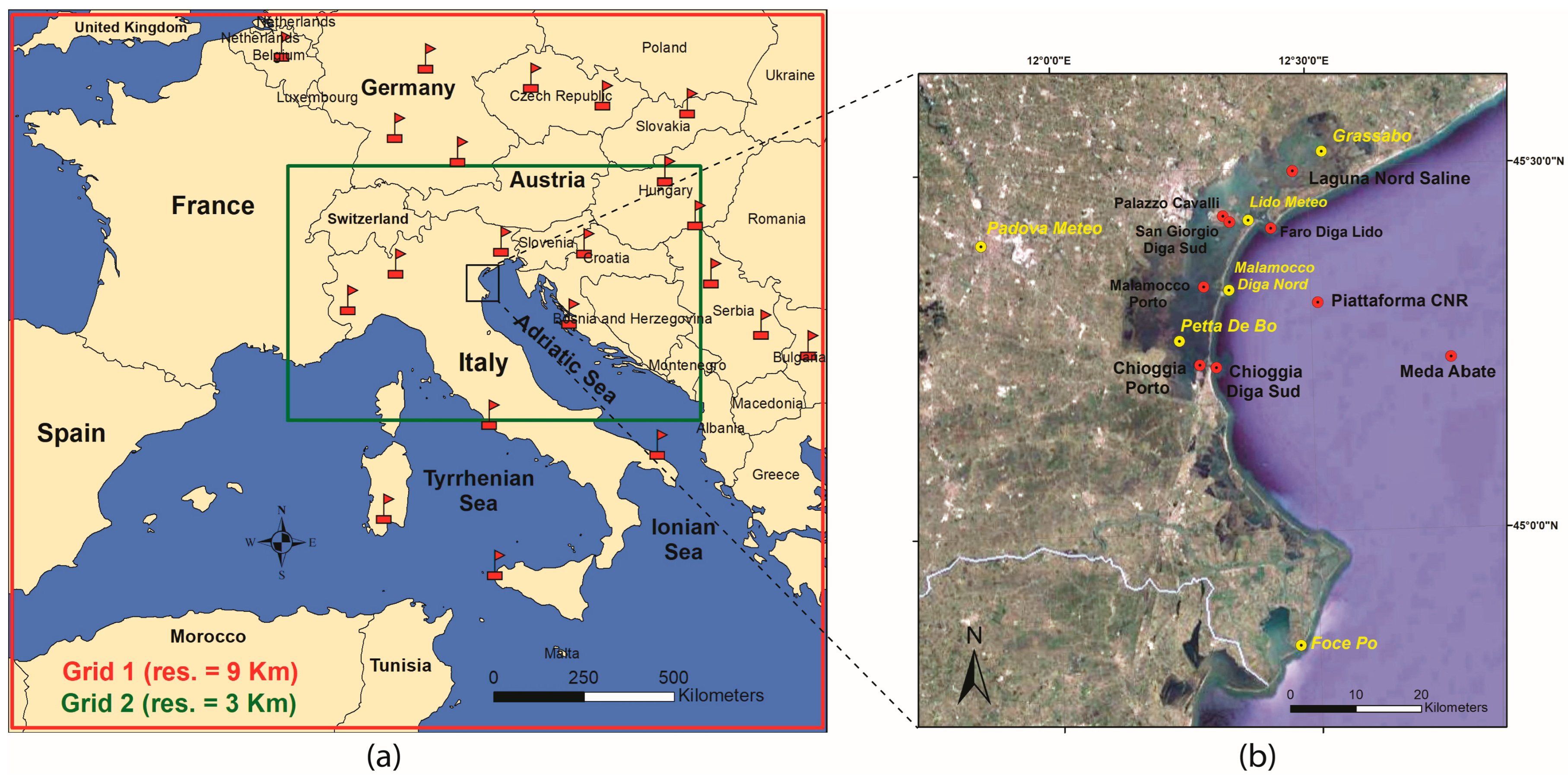
2.3. Data
3. Case Studies
3.1. Introduction
3.2. Case Study 1: 4 April 2019
3.2.1. Description
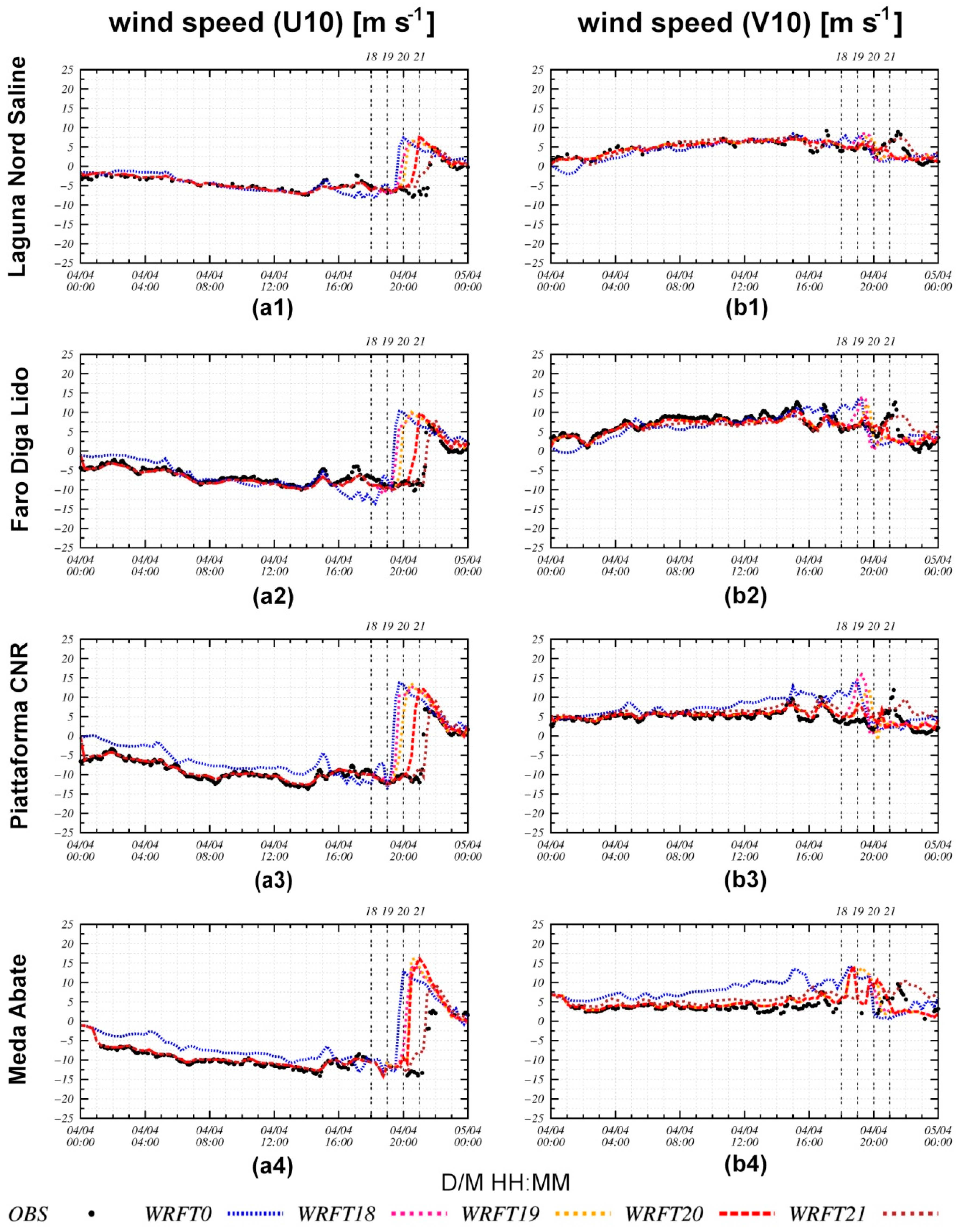
3.2.2. Results and Discussion
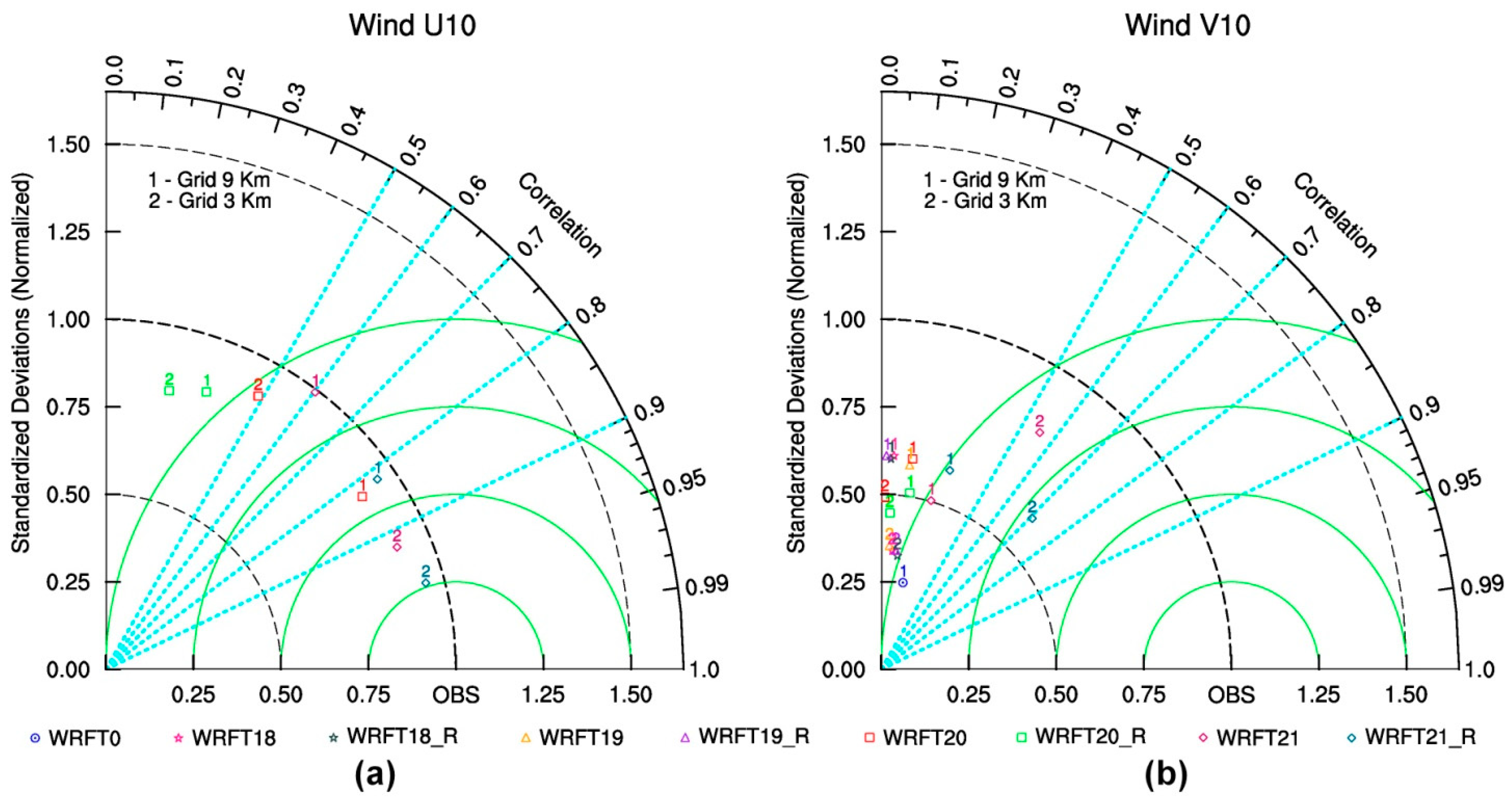
- (a)
- The correlation coefficient, related to the azimuthal angle in the diagram (dashed cyan radial lines), measures the pattern similarity between the simulated and observed fields;
- (b)
- The normalized standard deviation, proportional to the radial distance from the origin (dashed black contours), indicates the relative amplitude of the model and observed variations;
- (c)
- The centered root-mean-square error in the simulated field is proportional to the distance between each mark and the point on the x-axis identified as “OBS” (green contours). It is a measure of how realistically each simulation (and each grid) reproduces the observations, independently of the model bias.
3.3. Case study 2: 12 November 2019
3.3.1. Description
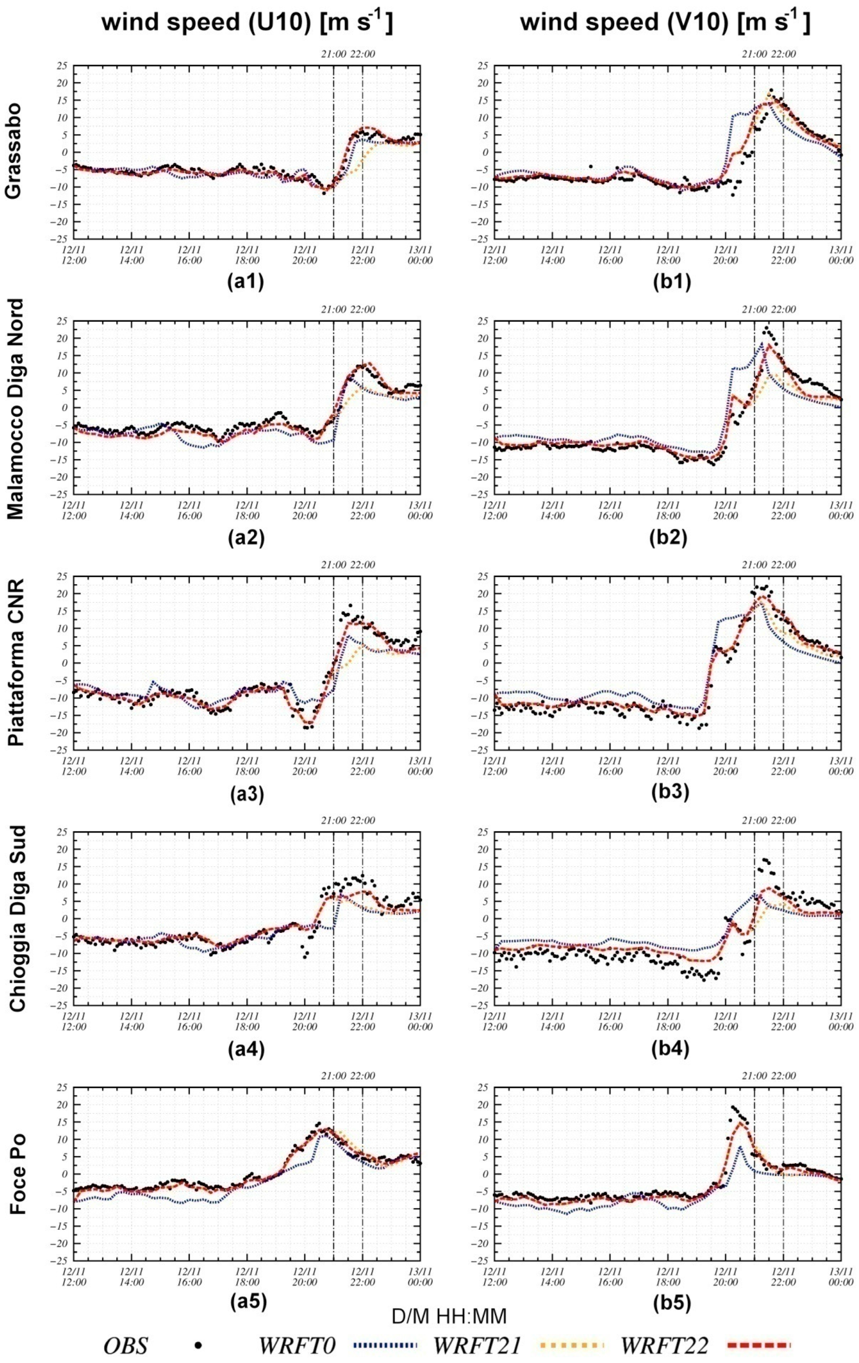
3.3.2. Results and Discussion
4. Conclusions
Author Contributions
Funding
Institutional Review Board Statement
Informed Consent Statement
Data Availability Statement
Acknowledgments
Conflicts of Interest
Appendix A

| A | B | |||
|---|---|---|---|---|
| d01 (9 km) | d02 (3 km) | d01 (9 km) | d02 (3 km) | |
| obs_twindo (h) | 0.667 | 0.4 | 0.667 | 0.667 |
| obs_rinxy (km) | 75 | 20 | 75 | 20 |
| obs_sfcfact | 1 | 1 | 0.083 | 0.083 |
| obs_dtramp (min) | 0 | 0 | 60 | 60 |
| fdda_end (min) | 99,999 | 99,999 | 600 | 600 |
| obs_coef_wind (s−1) | 7.0 × 10⁻³ | 8.0 × 10⁻³ | 7.0 × 10⁻³ | 8.0 × 10⁻³ |
| obs_coef_temp (s−1) | 7.0 × 10⁻³ | 8.0 × 10⁻³ | 7.0 × 10⁻³ | 8.0 × 10⁻³ |
| obs_coef_mois (s−1) | 7.0 × 10⁻³ | 8.0 × 10⁻³ | 7.0 × 10⁻³ | 8.0 × 10⁻³ |

References
- Nicholls, R.J.; Wong, P.P.; Burkett, V.R.; Codignotto, J.O.; Hay, J.E.; McLean, R.F.; Ragoonaden, S.; Woodroffe, C.D. Coastal systems and low-lying areas. In Climate Change 2007: Impacts, Adaptation and Vulnerability. Contribution of Working Group II to the Fourth Assessment Report of the Intergovernmental Panel on Climate Change; Parry, M.L., Canziani, O.F., Palutikof, J.P., van der Linden, P.J., Hanson, C.E., Eds.; Cambridge University Press: Cambridge, UK, 2007; pp. 315–356. [Google Scholar]
- Woodworth, P.L.; Melet, A.; Marcos, M.; Ray, R.D.; Wöppelmann, G.; Sasaki, Y.N.; Cirano, M.; Hibbert, A.; Huthnance, J.M.; Monserrat, S.; et al. Forcing Factors Affecting Sea Level Changes at the Coast. Surv. Geophys. 2019, 40, 1351–1397. [Google Scholar] [CrossRef] [Green Version]
- Vilibić, I.; Šepić, J.; Pasarić, M.; Orlić, M. The Adriatic Sea: A long-standing laboratory for sea level studies. Pure Appl. Geophys. 2017, 174, 3765–3811. [Google Scholar] [CrossRef]
- Vilibić, I.; Denamiel, C.; Zemunik, P.; Monserrat, S. The Mediterranean and Black Sea meteotsunamis: An overview. Nat. Hazards 2020, 106, 1223–1267. [Google Scholar] [CrossRef]
- Lionello, P.; Nicholls, R.J.; Umgiesser, G.; Zanchettin, D. Venice flooding and sea level: Past evolution, present issues, and future projections (introduction to the special issue). Nat. Hazards Earth Syst. Sci. 2021, 21, 2633–2641. [Google Scholar] [CrossRef]
- Umgiesser, G. The impact of operating the mobile barriers in Venice (MOSE) under climate change. J. Nat. Conserv. 2020, 54, 125783. [Google Scholar] [CrossRef]
- Ferrarin, C.; Bajo, M.; Benetazzo, A.; Cavaleri, L.; Chiggiato, J.; Davison, S.; Davolio, S.; Lionello, P.; Orlić, M.; Umgiesser, G. Local and large-scale controls of the exceptional Venice floods of November 2019. Prog. Oceanogr. 2021, 197, 102628. [Google Scholar] [CrossRef]
- Ferrarin, C.; Lionello, P.; Orlić, M.; Raicich, F.; Salvadori, G. Venice as a paradigm of coastal flooding under multiple compound drivers. Sci. Rep. 2022, 12, 5754. [Google Scholar] [CrossRef] [PubMed]
- Miglietta, M.M.; Buscemi, F.; Dafis, S.; Papa, A.; Tiesi, A.; Conte, D.; Davolio, S.; Flaounas, E.; Levizzani, V.; Rotunno, R. A high-impact meso-beta vortex in the Adriatic Sea. QJRMS 2023. [Google Scholar] [CrossRef]
- Skamarock, W.C.; Klemp, J.B.; Dudhia, J.; Gill, D.O.; Liu, Z.; Berner, J.; Wang, W.; Powers, J.G.; Duda, M.G.; Barker, D.M.; et al. A Description of the Advanced Research WRF Model Version 4; No. NCAR/TN-556+STR; National Center for Atmospheric Research: Boulder, CO, USA, 2019. [Google Scholar]
- Thompson, G.; Field, P.R.; Rasmussen, R.M.; Hall, W.D. Explicit forecasts of winter precipitation using an improved bulk microphysics scheme. Part II: Implementation of a new snow parameterization. Mon. Weather Rev. 2008, 136, 5095–5115. [Google Scholar] [CrossRef]
- Mlawer, E.J.; Taubman, S.J.; Brown, P.D.; Iacono, M.J.; Clough, S.A. Radiative transfer for inhomogeneous atmospheres: RRTM, a validated correlated-k model for the longwave. J. Geophys. Res. 1997, 102, 16663–16682. [Google Scholar] [CrossRef] [Green Version]
- Dudhia, J. Numerical study of convection observed during the Winter Monsoon experiment using a mesoscale two-dimensional model. J. Atmos. Sci. 1989, 46, 3077–3107. [Google Scholar] [CrossRef]
- Jiménez, P.A.; Dudhia, J.; González-Rouco, J.F.; Navarro, J.; Montávez, J.P.; García-Bustamante, E. A revised scheme for the wrf surface layer formulation. Mon. Weather Rev. 2012, 140, 898–918. [Google Scholar] [CrossRef] [Green Version]
- Fairall, C.W.; Bradley, E.F.; Hare, J.E.; Grachev, A.A.; Edson, J.B. Bulk parameterization of air-sea fluxes: Updates and verification for the COARE algorithm. J. Clim. 2003, 16, 571–591. [Google Scholar] [CrossRef]
- Tewari, M.; Chen, F.; Wang, W.; Dudhia, J.; LeMone, M.A.; Mitchell, K.; Ek, M.; Gayno, G.; Wegiel, J.; Cuenca, R.H. Implementation and verification of the unified NOAH land surface model in the WRF model. In Proceedings of the 20th Conference on Weather Analysis and Forecasting/16th Conference on Numerical Weather Prediction, Seattle, WA, USA, 12–16 January 2004; American Meteorological Society: Boston, MA, USA, 2004. [Google Scholar]
- Hong, S.-Y.; Lim, J.-O.J. The WRF single-moment 6-class microphysics scheme (WSM6). J. Korean Meteorol. Soc. 2006, 42, 129–151. [Google Scholar]
- Kain, J.S. The Kain–Fritsch convective parameterization: An update. J. Appl. Meteorol. 2004, 43, 170–181. [Google Scholar] [CrossRef]
- Reen, B. A Brief Guide to Observation Nudging in WRF, Battlefield Environment Division, Army Research Laboratory February 2016. Available online: https://www2.mmm.ucar.edu/wrf/users/docs/ObsNudgingGuide.pdf (accessed on 1 February 2020).
- Chen, D.S.; Hsiao, L.F.; Xie, J.H.; Peng, M.S.; Fong, C.T.; Chang, P.L.; Fang, W.T.; Hong, J.S.; Yeh, T.C. Impacts of assimilating dual-doppler radar-retrieval winds on the twrf predictions of typhoon Nesat (2017). Terr. Atmos. Ocean. Sci. 2021, 32, 649–667. [Google Scholar] [CrossRef]
- Sun, H.; Wang, H.; Yang, J.; Zeng, Y.; Zhang, Q.; Liu, Y.; Gu, J.; Huang, S. Improving Forecast of Severe Oceanic Mesoscale Convective Systems Using FY-4A Lightning Data Assimilation with WRF-FDDA. Remote Sens. 2022, 14, 1965. [Google Scholar] [CrossRef]
- Taylor, K.E. Summarizing multiple aspects of model performance in a single diagram. Atmospheres 2001, 106, 7183–7192. [Google Scholar] [CrossRef]


| Date | Height (cm) | Date | Height (cm) |
|---|---|---|---|
| 16 April 1936 | 147 | 16 November 2002 | 147 |
| 12 November 1951 | 151 | 1 December 2008 | 156 |
| 15 October 1960 | 145 | 23 December 2009 | 144 |
| 4 November 1966 | 194 | 25 December 2009 | 145 |
| 3 November 1968 | 144 | 24 December 2010 | 144 |
| 17 February 1979 | 140 | 1 November 2012 | 143 |
| 22 December 1979 | 166 | 11 November 2012 | 149 |
| 1 February1986 | 158 | 12 February 2013 | 143 |
| 8 December 1992 | 142 | 29 October 2018 | 156 |
| 6 November 2000 | 144 | 12 November 2019 | 187 1 |
| Simulations List | ||||||||||
|---|---|---|---|---|---|---|---|---|---|---|
| Case Study | Simulation Name | Time Start (UTC) | Length (hours) | FDDA Grid 9 km | FDDA Grid 3 km | Time FDDA Turned off (UTC) | Reduced Acquisition Time Window | Horizontal Radius of Influence (km) | Type of Nesting | obs_coef_wind |
| 4 April 2019 | WRFT0 | 00:00 | 24 | OFF | OFF | 00:00 | NO | 75, 20 | One Way | 7 × 10⁻³, 8 × 10⁻³ |
| WRFT20_rinxy1 | 00:00 | 24 | ON | ON | 20:00 | NO | 35, 10 | One Way | 7 × 10⁻³, 8 × 10⁻³ | |
| WRFT20_rinxy2 | 00:00 | 24 | ON | ON | 20:00 | NO | 25, 6 | One Way | 7 × 10⁻³, 8 × 10⁻³ | |
| WRFT20_G1OFF_G2ON_TW | 00:00 | 24 | OFF | ON | 20:00 | NO | 75, 20 | Two Way | 7 × 10⁻³, 8 × 10⁻³ | |
| WRFT20_G1OFF_G2ON_TW_R | 00:00 | 24 | OFF | ON | 20:00 | YES | 75, 20 | Two Way | 7 × 10⁻³, 8 × 10⁻³ | |
| WRFT20_G1ON_G2OFF | 00:00 | 24 | ON | OFF | 20:00 | NO | 75, 20 | One Way | 7 × 10⁻³, 8 × 10⁻³ | |
| WRFT20_G1ON_G2OFF_R | 00:00 | 24 | ON | OFF | 20:00 | YES | 75, 20 | One Way | 7 × 10⁻³, 8 × 10⁻³ | |
| WRFT20_G1OFF_G2ON | 00:00 | 24 | OFF | ON | 20:00 | NO | 75, 20 | One Way | 7 × 10⁻³, 8 × 10⁻³ | |
| WRFT20_G1OFF_G2ON_R | 00:00 | 24 | OFF | ON | 20:00 | YES | 75, 20 | One Way | 7 × 10⁻³, 8 × 10⁻³ | |
| WRFT20_W | 00:00 | 24 | OFF | ON | 20:00 | NO | 75, 20 | One Way | 6 × 10⁻⁴, 6 × 10⁻⁴ | |
| WRFT18 | 00:00 | 24 | ON | ON | 18:00 | NO | 75, 20 | One Way | 7 × 10⁻³, 8 × 10⁻³ | |
| WRFT18_R | 00:00 | 24 | ON | ON | 18:00 | YES | 75, 20 | One Way | 7 × 10⁻³, 8 × 10⁻³ | |
| WRFT19 | 00:00 | 24 | ON | ON | 19:00 | NO | 75, 20 | One Way | 7 × 10⁻³, 8 × 10⁻³ | |
| WRFT19_R | 00:00 | 24 | ON | ON | 19:00 | YES | 75, 20 | One Way | 7 × 10⁻³, 8 × 10⁻³ | |
| WRFT20 | 00:00 | 24 | ON | ON | 20:00 | NO | 75, 20 | One Way | 7 × 10⁻³, 8 × 10⁻³ | |
| WRFT20_R | 00:00 | 24 | ON | ON | 20:00 | YES | 75, 20 | One Way | 7 × 10⁻³, 8 × 10⁻³ | |
| WRFT21 | 00:00 | 24 | ON | ON | 21:00 | NO | 75, 20 | One Way | 7 × 10⁻³, 8 × 10⁻³ | |
| WRFT21_R | 00:00 | 24 | ON | ON | 21:00 | YES | 75, 20 | One Way | 7 × 10⁻³, 8 × 10⁻³ | |
| 12 November 2019 | WRFT0 | 12:00 | 12 | ON | ON | 12:00 | NO | 75, 20 | One Way | 7 × 10⁻³, 8 × 10⁻³ |
| WRFT21 | 12:00 | 12 | ON | ON | 21:00 | NO | 75, 20 | One Way | 7 × 10⁻³, 8 × 10⁻³ | |
| WRFT21_R | 12:00 | 12 | ON | ON | 21:00 | YES | 75, 20 | One Way | 7 × 10⁻³, 8 × 10⁻³ | |
| WRFT22 | 12:00 | 12 | ON | ON | 22:00 | NO | 75, 20 | One Way | 7 × 10⁻³, 8 × 10⁻³ | |
| WRFT22_R | 12:00 | 12 | ON | ON | 22:00 | YES | 75, 20 | One Way | 7 × 10⁻³, 8 × 10⁻³ | |
Disclaimer/Publisher’s Note: The statements, opinions and data contained in all publications are solely those of the individual author(s) and contributor(s) and not of MDPI and/or the editor(s). MDPI and/or the editor(s) disclaim responsibility for any injury to people or property resulting from any ideas, methods, instructions or products referred to in the content. |
© 2023 by the authors. Licensee MDPI, Basel, Switzerland. This article is an open access article distributed under the terms and conditions of the Creative Commons Attribution (CC BY) license (https://creativecommons.org/licenses/by/4.0/).
Share and Cite
Conte, D.; Tiesi, A.; Cheng, W.; Papa, A.; Miglietta, M.M. Nowcasting of Wind in the Venice Lagoon Using WRF-FDDA. Atmosphere 2023, 14, 502. https://doi.org/10.3390/atmos14030502
Conte D, Tiesi A, Cheng W, Papa A, Miglietta MM. Nowcasting of Wind in the Venice Lagoon Using WRF-FDDA. Atmosphere. 2023; 14(3):502. https://doi.org/10.3390/atmos14030502
Chicago/Turabian StyleConte, Dario, Alessandro Tiesi, Will Cheng, Alvise Papa, and Mario Marcello Miglietta. 2023. "Nowcasting of Wind in the Venice Lagoon Using WRF-FDDA" Atmosphere 14, no. 3: 502. https://doi.org/10.3390/atmos14030502