Article

Seasonal Field Calibration of Low-Cost PM2.5 Sensors in Different Locations with Different Sources in Thailand

1
Air Pollution and Health Effect Research Center, Prince of Songkla University, Songkhla 90110, Thailand
2
Department of Chemical Engineering, Faculty of Engineering, Prince of Songkla University, Songkhla 90110, Thailand
3
Department of Mechanical and Mechatronics Engineering, Faculty of Engineering, Prince of Songkla University, Songkhla 90110, Thailand
4
Faculty of Engineering and Technology, King Mongkut’s University of Technology North Bangkok, Bankhai, Rayong 21120, Thailand
5
Department of Computer Engineering, Faculty of Engineering, Prince of Songkla University, Songkhla 90110, Thailand
6
Institute of Environmental Engineering, National Yang Ming Chiao Tung University, Hsinchu 300093, Taiwan
7
Department of Environmental Science and Engineering, Tunghai University, Taichung 407224, Taiwan
8
School of Industrial Engineering and Technology, King Mongkut’s Institute of Technology Latkrabang, Bangkok 10520, Thailand
*
Author to whom correspondence should be addressed.
Atmosphere 2023, 14(3), 496; https://doi.org/10.3390/atmos14030496
Submission received: 30 January 2023 / Revised: 24 February 2023 / Accepted: 1 March 2023 / Published: 3 March 2023
(This article belongs to the Section Air Quality)

Abstract

:
Low-cost sensors (LCS) have been increasingly deployed to monitor PM2.5 concentrations. More than 1500 LCS have been installed in Thailand to increase public awareness of air quality. However, performance of these sensors has not been systematically investigated. In this study, PM2.5 LCS were co-located next to a PM2.5 federal equivalent method (FEM) reference instrument at three Thai locations—in the north, center and northeast. We evaluated the performance of a PM2.5 LCS (PMS7003, Plantower) to understand the key factors affecting performance, including emission sources, relative humidity, temperature and PM2.5 concentration. Low PM concentration and high humidity levels had a significant impact on performance. Sensors in a high traffic emission area showed low correlation. The unadjusted PM2.5 LCS performance varied with locations. Errors were mainly observed at low concentrations. They significantly underestimated concentrations in congested urban environments. After calibration, accuracy was improved with multiple regression models. The performance of sensors only at Chiang Mai (CM) during the dry season and Ubon Ratchathani (URT) during the dry and wet seasons were acceptable with coefficient of variation: 5.8 ± 4.7–6.8 ± 5.0%, slope: 0.829–0.945, intercept: 1.12–5.49 µg/m3, R2: 0.880–0.934 and RMSE: 4.3–5.1 µg/m3. In the congested area in Bangkok (BKK), they underestimated concentrations of small particles.

1. Introduction

Air pollutants in many countries in Southeast Asia are influenced from diverse sources. In Thailand, the major sources are vehicles, industry, long-range transport, secondary aerosol formation as well as open biomass burning [1,2,3,4,5,6,7,8,9,10,11]. Traffic is the most influential factor on air quality in the capital city of Bangkok, though some studies indicated that biomass burning was the major cause of atmospheric aerosols during the dry period [6,7,12]. Air quality in northern Thailand was annually affected by domestic and transboundary sources as a result of forest fires and agriculture waste burning during the dry season [1,3,9]. Agricultural area in Thailand covers 24 M ha or 46.5% of the total land [13]. The northeastern region is the largest agricultural area (~10 M ha), followed by the northern and central regions [14]. Normally, agricultural waste has been burned in the open for clearing and preparing for the next crop [15]: January to April is the biomass intensive burning period, not only in Thailand, but also in other countries in the Mekong Subregion, including Laos, Cambodia, Vietnam and Myanmar [2]. All these events cause Thailand serious and long-term air pollution problems, particularly fine particles or PM2.5. Though the standard for PM2.5 in Thailand has been enforced since 2010, it was not until recently that there has been strong public awareness: the advent and widespread use of low-cost and easily acquired PM2.5 sensors contributed to this.
Air quality monitoring networks in Thailand have been established by the Pollution Control Department (PCD) to monitor the air pollutants, including PM10, PM2.5 and noxious gases (CO, NO2, SO2 and O3). PCD started to monitor ambient PM2.5 concentrations in 2011 with only three monitoring stations in three Thai megacities—Rayong, Chiang Mai and Bangkok. National allowable ambient PM2.5 concentrations in Thailand were set on 28 Jan 2010, with the average 24-h concentration not to exceed 50 µg/m3 [16]. Currently, ambient PM2.5 concentrations monitoring stations have been expanded to more than 77 stations in 45 cities [16]. However, the FEM instruments [17], such as the tapered element oscillating microbalance (TEOM) and the beta attenuation monitor (BAM), are still relatively expensive and they are only deployed at central monitoring sites in each province. One monitors station cannot represent the correct spatial PM2.5 concentrations [18,19,20,21].
Low-cost sensors (LCS) for air quality monitoring have been widely used in recent years to fill gaps in the existing air quality monitoring networks and provide the public with locally relevant particle concentrations, especially PM2.5, in real time, at much higher spatial and temporal resolutions. At present, LCS have been deployed to monitor PM2.5 concentrations, with more than 1500 monitoring stations installed in Thailand [22]. In general, the performance of the PM2.5 LCS showed a high correlation relative to FEM instruments (R2 > 0.85) in the laboratory under controlled conditions [19,21,23,24,25]. However, typically, they were less accurate in the field, where correlations were found in the range 0.36 ≤ R2 ≤ 0.99 [20,21,26,27,28,29], with variations due to sources, particle sizes and shapes, compositions and concentrations [30]. The different meteorological conditions, including temperature and relative humidity (RH), also influenced LCS performance (20). Therefore, a PM2.5 LCS calibrated under laboratory condition may not be suitable for direct field measurements [21,27,31].
Calibration of LCS is necessary due to both the physical and chemical characteristics of aerosols [32] and meteorological conditions [28,33]. Levy Zamora et al. [32] evaluated three Plantower PMSA003 sensors exposed to eight PM sources, including incense, oleic acid, NaCl, talcum powder, cooking emissions and monodispersed polystyrene latex spheres, under controlled laboratory conditions. The accuracy ranged from 13% to >90% compared with reference instruments; hence, PM sources influenced LCS performance. The LCS were most accurate for sizes < 1 μm. Additionally, meteorological conditions, including temperature and RH, significantly influenced LCS performance [28,33]. Levy Zamora et al. [32] showed that the LCS error increased at higher RH levels (greater than 80%) in the field. Jayarathne et al. [33] also found that the LCS mass concentrations were at least 80% higher than the FEM values at high RH levels (78–89%). Additionally, Levy Zamora et al. [32] showed that an RH level > 50% deceased the accuracy of the LCS. Therefore, they need to be calibrated under realistic ambient conditions before deployed for ambient PM2.5 monitoring.
A common approach for field calibration of the LCS is to collocate the LCS with an FEM/federal reference method (FRM) instrument and use mathematical models to adjust the LCS data to reference data [34,35]. Regression model is one of the earliest methods for LCS calibration [28,31,35]. Moreover, the machine learning (ML) methods were recently applied to improve the accuracy of the linear regression [34,36]. However, regression models including linear regression (LR), multi-linear regression (MLR) and nonlinear regression (NLR) are still widely used to calibrate the LCS, because of their simplicity and ease of implementation [35]. Zheng et al. [28] developed calibration models to improve the LCS performance against an FEM by using the LR, MLR and NLR based on PM2.5 concentration, temperature and RH in India. Zusman et al. [31] also developed an MLR calibration model based on the same parameters. The model showed the moderate accuracy for LCS versus the reference with R2 values in the range 0.67–0.84. Hong et al. [21] developed a set of models based on LR, MLR and NLR to correct the PM2.5 concentration from LCS in Taiwan: they found that NLR methods were superior to LR. Barkjohn et al. [37] proposed an MLR calibration model, based on PM2.5 concentration and RH, to be used as a US-wide correction model for the Purple Air sensors. Though the LCS performance has been studied in many countries, including India [28], Korea [38], Taiwan [21] and the USA [37], the studies of performance of PM2.5 LCS for field measurements in Thailand are limited and not well understood, especially related to locations and seasonal conditions.
This study adds new insights to understanding the key factors affecting the performance of LCS, including relative humidity, temperature and PM2.5 concentration. The tested sensors had been operating for a long-term period, 15–16 months, at different locations in Thailand. In addition, LCS calibration based on reference concentrations, RH and temperature levels by using linear regression (LR) and multiple linear regression (MLR) models were also investigated to improve the PM2.5 LCS performance so that it became an acceptable suppletory means for public monitoring of PM2.5 concentration. This will help to increase public awareness on air quality, which directly affects their health.

2. Materials and Methods

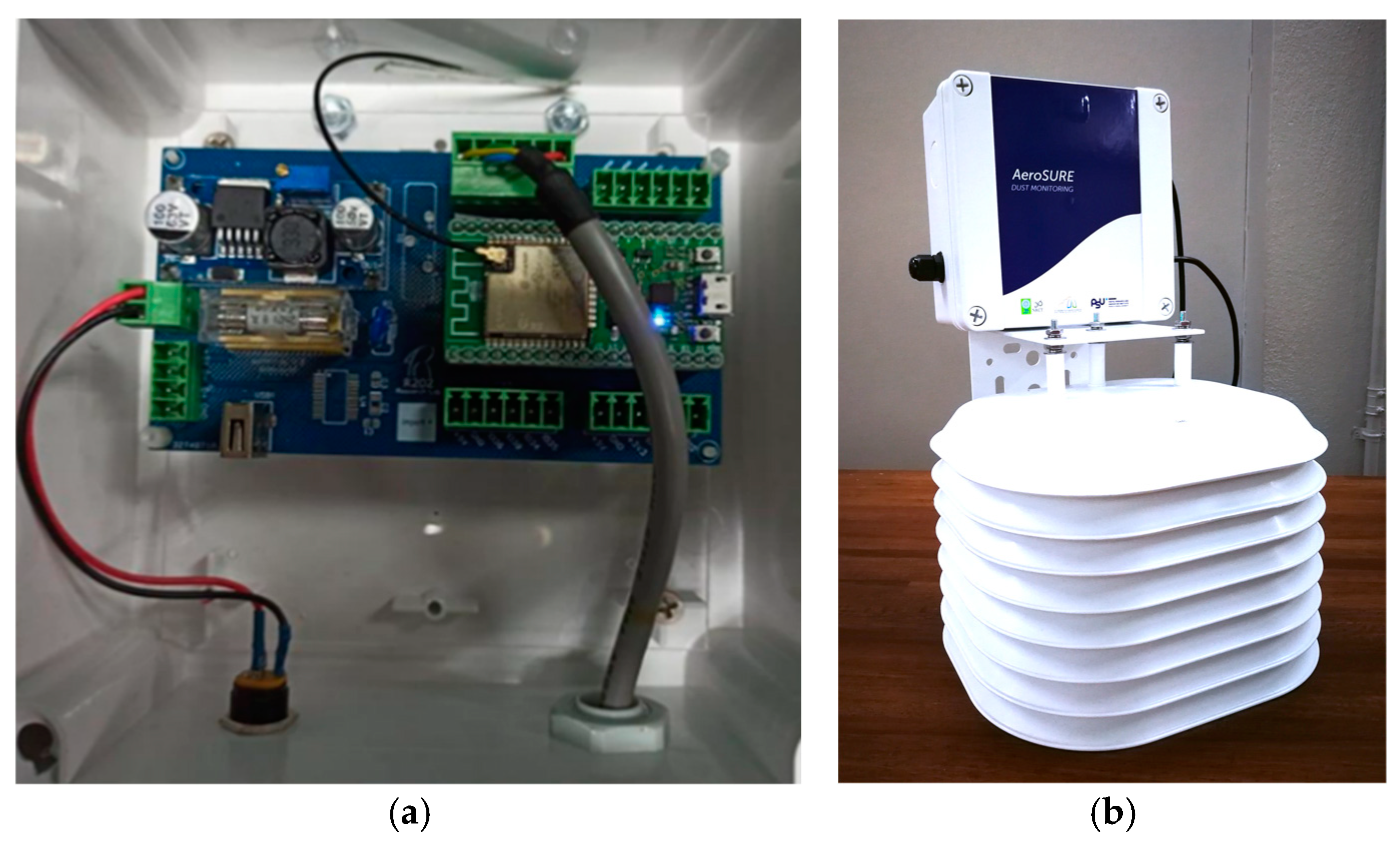
2.1. The Low-Cost PM2.5 Sensors

In the present study, the particulate matter low-cost sensors used for field calibration were made by Plantower (model PMS7003) equipped with custom-designed electric circuit and a housing as shown in Figure 1. The PMS7003 used a light-scattering technique to measure real-time PM mass concentrations [26]. The PM2.5 measurement range was 0–1000 µg/m3, with a resolution of ±1 µg/m3 and response time 1–10 s, provided by the manufacturer [39]. The dimension of the miniature sensor used was 48 mm × 37 mm × 12 mm. The manufacturer reported that maximum errors were relatively low (±10 µg/m3 for <100 µg/m3 concentrations and ±10% for 100–500 µg/m3 concentrations). The RH and temperature for calibration were measured by thermo-hygrometer (LSI LASTEM, DMA875) at each monitoring site. The primary sensor reported data include PM1, PM2.5, and PM10 concentrations with a factory-specified correction factor for ambient measurement concentrations (CF = atm), as recommended by the manufacturer. The description of the selected low-cost PM2.5 sensors (LCS) in the present study was mentioned in a field evaluation study of PM2.5 [40].
In the PMS low-cost sensor, the raw PM2.5 mass concentration was obtained by converting particle number concentrations from different particle size bins. The effect of number-to-mass conversion on the performance of the PMS5003 was studied by Hong et al. [21]. A good correlation between the measured number concentration and the raw PM2.5 mass concentration (R2 = 0.99) was found, but a high conversion ratio was needed. This indicated that using the measured number concentrations from different size bins for calibration can provide similar results to the use of raw PM2.5 concentrations. In this study, we used the PMS7003, which is expected to perform similarly to the PMS5003 because it has the same particle size bins [39,41]. Additionally, a field test confirmed the similar performance of the two sensors compared to the PM2.5 FEM monitor [42]. Therefore, the effects of the measured number concentrations from different size bins on the performance of the PMS7003 can be considered negligible.

2.2. Sampling Locations and Periods

The low-cost PM2.5 sensors were placed at three PCD monitoring stations in Chiang Mai (CM) in the north, Bangkok (BKK) in central and Ubon Ratchathani (URT) in the northeast of Thailand—see Table 1 and Figure 2. Three identical LCS were located next to the PM2.5 FEM instrument sampling probe on the rooftop of each PCD station (~3 m above ground). The FEM instruments were a BAM-1020 (Met One, Grants Pass, OR, USA) at the CM site, an MP101M (ENVEA, Poissy, France) at the BKK site and a T640 (Teledyne, Thousand Oaks, CA, USA) at the URT site. Key specifications of these instruments and the test periods are in Table 1: brief descriptions of the FEMs are in [21]. The FEM instrument at URT was calibrated to the FRM by the National Institute of Metrology (Thailand) [43]; the correlation between FEM and FRM was acceptable with regression equation: y = 1.084x + 4.093 (R2 = 0.94). The data from FEM instruments were collected and provided by PCD. The LCS data were transmitted in real time to our server. The PM2.5 FEM instruments also monitor meteorological parameters, including ambient temperature and relative humidity, and they were used in our LCS calibration. Weather in Thailand is influenced by two monsoon seasons: the northeast monsoon from December to March and the southwest monsoon from May to October [44] and is usually described as falling into two seasons according to the rainfall: the dry season (November to April) and wet season (May to October) [45]. The location characteristics at each sampling site in all these regions is described below.
In the northern part of Thailand, LCS were placed at Chiang Mai municipal center, Chiang Mai (PCD station#35/CM). Chiang Mai is one of the largest and most famous cities in Upper Southeast Asia (SEA): the geography consists of high mountains along the north–south corridor, covered with forest (69.7%) and agricultural areas (23.7%) [46]. Its air pollution is normally influenced by domestic and transboundary sources, particularly forest fires, as well as agriculture waste burning during the dry season [2,9]. Temperature inversions in the winter enhance accumulation of the pollutants near the ground [9]. In central Thailand, LCS were placed at the National Housing Authority Public Community, Din Daeng District, Bangkok (PCD station#54/BKK): it is a business center, where traffic is among the worst in Bangkok, from normal to slow speed vehicles. In the northeast, LCS were placed in Ubon Ratchathani (PCD station#83/URT), a large province in northeast Thailand, bordering with Cambodia. It is an agricultural-based province, where rice paddy fields cover the major portion of the land [47]. The burned area from agricultural residue in Thailand was mainly found in the northeast [12,47]. Rice and sugarcane residue burning in the northeast contributes to 50% and 40% of total agricultural waste burned in Thailand [15,48]. Open burning of the agricultural waste, as well as transboundary haze from neighboring countries, leads to a high level of air pollution there.

2.3. Sensor Calibration

The parameters used in the calibrations of the low-cost PM2.5 sensors in the present study include the reference monitors, RH and temperature. First, hourly moving averaged PM2.5 concentrations from the LCS and the accompanying FEM, along with RH, and temperature were collected in a single dataset for each location; the number of data records are shown in Table 1. The LR and MLR terms were developed to improve the PM2.5 LCS—listed in Table 2. In those equations, PM 2.5 - FEM represents is the hourly PM2.5 concentration of the FEM measurement, Raw   PM 2.5 - LCS represents the PM2.5 concentration provided by the LCS and a j to i j are the fitted model coefficients and intercepts. Model#1 is the simple LR model based on only the PM2.5 concentration. Model#2–Model#4 are the MLR models with addition of T, RH and both T and RH. MLR models with additional product terms are Model#5 (add RH and RH and PM2.5 product), Model#6 (add T and RH and product of RH and PM2.5), Model#7 (add T and product of T and PM2.5), Model#8 (add T and RH and product of T and PM2.5) and Model#9 (addition of T and RH and multiplication of T, RH and PM2.5). We used the linear RH model because it had better performance than the nonlinear RH model [37]. However, we also included the nonlinear RH term, RH2/(1−RH), in the model for comparison. Details of the calculation were described by [28].

2.4. Performance Metrics

The performance of the LCS and FEM at each site were examined based on the U.S. EPA guidelines [43], including precision: coefficient of variation, CV ≤ 30%, bias: slope (1.0 ± 0.35) and intercept of 0 ± 5 µg/m3, linearity: coefficient of determination, R2 ≥ 0.7 and error: root mean square error, RMSE ≤ 7 µg/m3. A linear regression for LCS measurements compared to the reference instrument calculated the slope, intercept and R2 to represent the LCS accuracy.
Precision between identical sensors was characterized by coefficient of variation, calculated every hour by:
C V = S D x ¯ × 100
The root means square error, RMSE, was used to help understand the error associated with sensors for PM2.5 concentration measurements:
RMSE = 1 N × M j = 1 M t = 1 N ( x t , j y ¯ t ) 2
where SD is the standard deviation of averaged PM2.5 LCS concentration, x ¯ is the mean PM2.5 LCS concentration (µg/m3), N is the number of samples, M is number of identical LCS, x t , j is the PM2.5 LCS concentration of sample # j at time t (µg/m3) and y ¯ t is the PM2.5 FEM concentration at the same time (µg/m3).
Akaike’s information criterion (AIC) was used to determine the significance of the RH and temperature term in the MRL models [28]. The AIC values were used to select the best model and avoid parameter overfitting. A lower value between any comparative pair of models was preferred. The AIC was calculated from:
AIC = N   ×   ln ( Residual   Sum   of   Squares N ) + ( 2   ×   k )
where k is the number of parameters.

3. Results and Discussion

3.1. Source Characteristics of PM2.5 in Different Areas

The overall-averaged PM2.5 concentrations from FEM instruments, at all three sites, obtained from PCD during the year 2020–2022 are listed in Table 3. In general, the ambient conditions at all stations across Thailand were quite similar. The PM2.5 concentrations and characteristics could be different from season to season and site to site.
Hourly PM2.5 mass concentration from FEM measurement at CM during the dry season was as high as 246 µg/m3. The average concentration during the dry season was 38.3 ± 23.0, about two times as high as that during the wet season (16.0 ± 5.5 µg/m3). Northern Thailand is typically influenced by transboundary and domestic aerosols. Domestic sources of ambient PM in northern Thailand were mostly forest fires (>90% of total burned area in northern Thailand), especially during the dry season. They occurred mostly in deciduous dipterocarp forest national parks [9]. Aerosol transport from open biomass burning area in some parts of Myanmar and Laos also affected air quality in northern Thailand [1,3,9]. Moreover, temperature inversion plays an important role, leading to high accumulation of air pollutants during the winter months (November to March) in northern Thailand [2].
In BKK, the average PM2.5 concentration during the dry season was also approximately two times as high as that during the wet season. Average PM2.5 concentrations during the wet season were about 1.5 times higher than those at CM and URT. This is because the local emission sources, especially vehicle emissions, were uniformly high due to traffic congestion [8]. As well as vehicle and industrial emissions, local biomass burning and long-range transport from other countries also contributed to the PM2.5 concentrations during the dry season which were 2–4 times as high as those in background [6,7]. Hence, fine particles in Bangkok came from diverse sources, including vehicle emissions, biomass burning, industrial, construction activities and secondary aerosols [6].
PM levels at URT were significantly enhanced by agricultural waste burning, especially rice and sugarcane, during the dry season. The northeastern region is the largest agricultural area (~10 M ha or 42% of the total). Most agricultural waste was burned in the open, for land clearing and preparing for the next crop, during January to April [15]. PM2.5 concentrations during the dry season (as high as 322 µg/m3) were higher than those in CM and BKK.

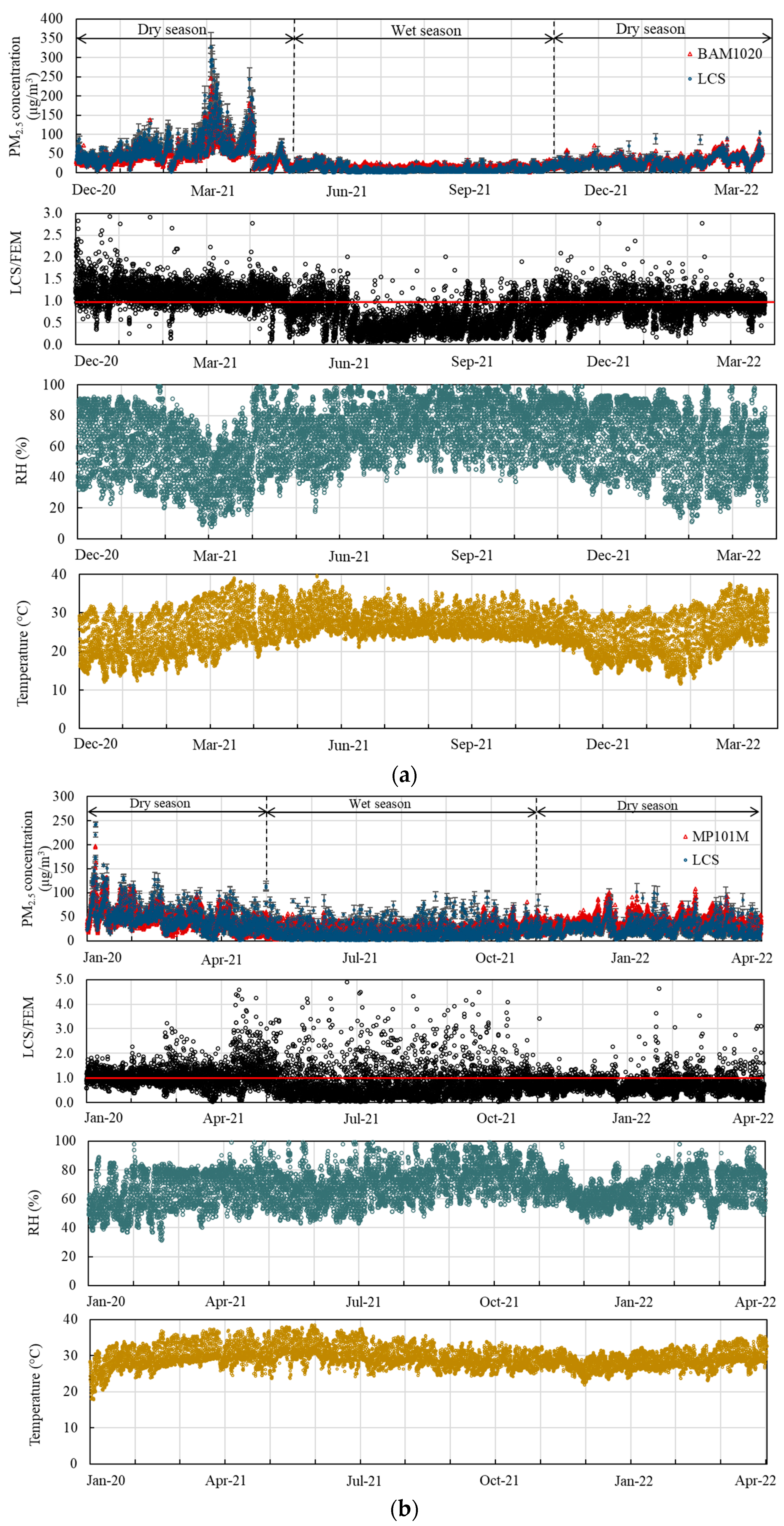
3.2. Time Series of PM2.5 Concentrations, Ratio of LCS and FEM, RH and Temperature

Figure 3 shows the seasonal variation of 1-h PM2.5 concentration from LCS and FEM, ratio of LCS to FEM, RH and temperature at all three sites. Overall, the uncalibrated LCS measurements mostly followed the trend in PM2.5 FEM measurements and responded well to most sudden spikes of mass concentrations. LCS to FEM ratios and meteorological factors (RH and temperature) are also summarized in Table 3. The LCS/FEM ratio during the dry season at CM and URT were close to 1, whereas it was lower at BKK. This indicated that the 1-h averaged ambient PM2.5 levels of uncalibrated LCS at CM and URT matched well, in general, to those obtained from the FEM instruments. However, PM2.5 LCS concentrations at URT during the dry season were lower than those from the T640. This agrees with Hagler et al. [49], who reported that the PM2.5 concentrations from a T640, an optically based FEM, closely matched those from a BAM-1020 instrument at lower concentrations, but overestimated concentrations above ~80 µg/m3. Average RH and temperature during the dry season ranged from 60 ± 15 to 66 ± 12% and 24.4 ± 5.4 to 29.0 ± 2.7 °C, respectively. Average RH during the wet season was significantly higher than those during the dry season (RH increased 9–24%), while temperature was also slightly higher. Average temperatures at CM and URT in the dry season were lower, because it included the winter months (Nov–Feb).
However, the LCS measurements also followed the FEM instruments during the wet season, except at BKK. The ratio of LCS/FEM using the beta ray technique, during the wet season at CM and BKK, were strongly lower than 1. Zheng et al. [28] showed that the LCS performance decreased with low PM2.5 concentration and high RH. This indicated that the LCS were highly sensitive to RH but in varying directions [50]. At BKK, the ratios of LCS/FEM were lower than 1 during both periods. This could be because the LCS at this site were located close to major roads in a highly congested area. Most of the particles from fresh traffic emissions were smaller than the LCS minimum detectable size (see detail in Section 3.5). This is consistent with Castell et al. [30], who reported that the LCS measurements, where traffic emission was low, were better correlated with the reference measurements. In contrast, the mean ratio of LCS/FEM during the wet season at URT was higher than 1 (1.2 ± 0.5). The ratio of LCS to FEM higher than 1.2 during the wet season, accounting for 53%, was found at high RH level (79 ± 12%). Moreover, we found that increased LCS errors (>1.7 ± 0.5) mostly occurred at the extreme RH level (84 ± 10%). This agrees with Zamora et al. (2019), who reported that the accuracy of LCS (Plantower PMSA003) decreased for RH > 50% [51,52]. Similarly, Jayarathne et al. [33] noted that the error of LCS increased for RH > 80%, in field monitoring. For the temperature effect, the temperature differential between dry and wet seasons at CM was as high as ~3 °C, while at BKK and URT it was closer to 1 °C—an insignificant change. Some reports have claimed that neither temperature or RH affected LCS errors [53,54]. However, others have noted that calibration to correct a temperature effect improved LCS, and our results (see later) show that temperature correction did improve accuracy [54].

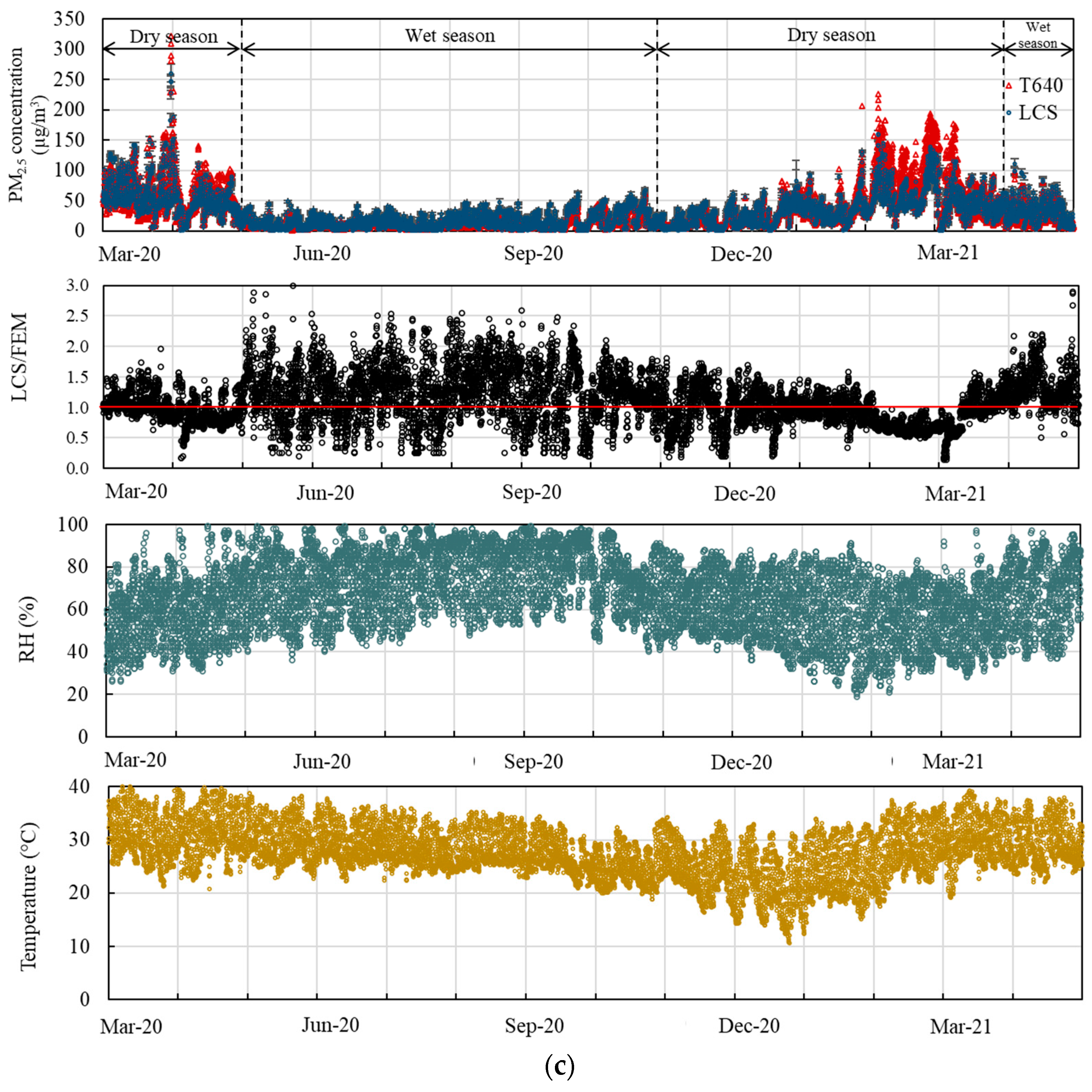
3.3. Influence of Concentration Range, RH and Temperature Levels on Sensor Performance

The distribution of the relative error of unadjusted LCS are shown in Figure 4. The relative error (%) values were calculated with 1-h averaged data of unadjusted PM2.5 LCS and FEM concentrations. For the concentration range, the highest relative errors for PM2.5 concentrations were observed below 20 µg/m3, while the maximum error values were up to 200%. For the CM and URT sites, between 20–50 μg/m3, the errors were mostly below 100% and they were mostly below 50% when the PM2.5 level went above 50 μg/m3. Values from LCS at BKK were mostly characterized by rather constant maximum relative errors at ~90% independent of the concentration range, RH or T (average: 40.2% for dry and 51.3% for wet). The highest relative errors were found during the wet season at all sites at low concentration (<20 µg/m3), with average PM2.5 concentrations of 16.1 ± 5.5 µg/m3 (CM), 23.6 ± 9.4 µg/m3 (BKK) and 15.4 ± 10.6 µg/m3 (URT). At CM, the relative error during the dry season was clearly increased at a higher RH level. This is consistent with the previous studies by Liu et al. [51] and Jayaratne et al. [33]. The relative error of LCS during the wet season doubled those in dry season at CM and URT. The error during the wet season at CM and BKK were nearly identical, with constant maximum ~90% at RH greater than 42%. The relative error of LSC at URT (average: 23.8% in dry season and 40.0% in wet season) was consistent with most previous studies, which showed that low PM concentration and RH level significantly impacted low-cost PM sensor performance [20,55,56,57]. However, it should be noted that Kosmopoulos et al. [29] reported that the effect of RH on the response of Plantower PMS5003 sensors for fine PM in southeast Europe was negligible, so the measurement location is important to consider. The relative errors of PM2.5 in the present study show no pattern for the influence of temperature levels on sensor performance. It is noted that beta attenuation monitor consists of the heater system with a controller to reduce the RH level of samples. It was normally set below a particular point to remove the hygroscopic and condensation effect of particles on the filter influencing the mass concentration reading. Hence, a range of RH set point is the critical factor to assess the performance of beta attenuation measurement [58,59]. Takahashi et al. [59] reported the PM concentration from BAM was higher than those using the gravimetric method at high RH (>80%). Kiss et al. [60] suggested that 1-h PM10 measurements must be used carefully, as water vapor adsorption/desorption from the beta attenuation monitor’s filter material may cause significant bias at low ambient concentration. Zheng et al. [28] also supported that the beta-attenuation-based monitors have drawbacks at low concentrations.

3.4. Responses of the LCS to Emission Sources

The response of the PM2.5 LCS to the different emission sources was interpreted in the present study (see Figure 5). The different R2 of linear regression results between PM2.5 concentrations from the LCS and the FEM instruments in locations where major aerosol sources were different indicated that the LCS had variable responses to types of aerosols. At BKK site, the LCS were located within a short distance from major roads, and the traffic emissions were mainly constituted of fresh vehicle exhaust as discussed in Section 3.1. The results showed that the R2 values of the linear regressions between LCS and FEM at BKK during the dry season (R2 = 0.561) were quite low, and very poor during the wet season (R2 = 0.291), in response to fresh vehicle exhaust emissions. However, the PM2.5 characteristics at BKK during the dry season were annually affected by domestic and transboundary aerosol transport from open biomass burning [6]. The R2 value of the linear regression between the LCS and the FEM was higher because of a large contribution from biomass burning. For CM and URT, R2 values of the regressions were high during the dry season in response to predominant open biomass burning. Not only does the emission source play a significant role, but ambient RH levels also had effects on the LCS performance. The LCS were more responsive to open biomass burning emissions than to fresh traffic emissions. This is because the particle size from diesel and gasoline engines were dominant in the range of 60–120 nm and 40–80 nm, respectively [61]. Hence, most of the particles from fresh traffic emissions were ultrafine particles (<0.1 µm), which are smaller than the minimum detectable size (0.3 µm) of the LCS. Moreover, the particle size from biomass burning were predominantly in the range of 0.5–2.5 µm [62]. Hata et al. [63] also reported that the dominant size of PM from biomass burning was in accumulation mode (PM0.5–1.0). This is why the linear regression between the PM2.5 LCS and FEM concentration at CM and URT were better than that at BKK, especially in dry season. This was confirmed by Sresawasd et al. [9], who reported the PM mass concentration was distributed mostly in the accumulation mode PM0.5–1 (38–48%) of TSP in Chiang Mai, Thailand during the haze period (dry season). Additionally, Dejchanchaiwong et al. [6] found that the PM0.5–1.0 concentrations in the haze period (Dec–Feb) were 2 to 12 times as high as those in the nonhaze period. However, underestimation of PM2.5 concentration may partly be a result from the limitation of the Plantower sensor. Kuula et al. [64] found that the large particle size fraction 1.0–2.5 µm significantly reduce the concentration of PM2.5 when using Plantower PMS5003. The finding of the LCS responses to different aerosol emission sources provided guidance on future application of LCS monitors, such as the distance of the deployment sites to major roads.

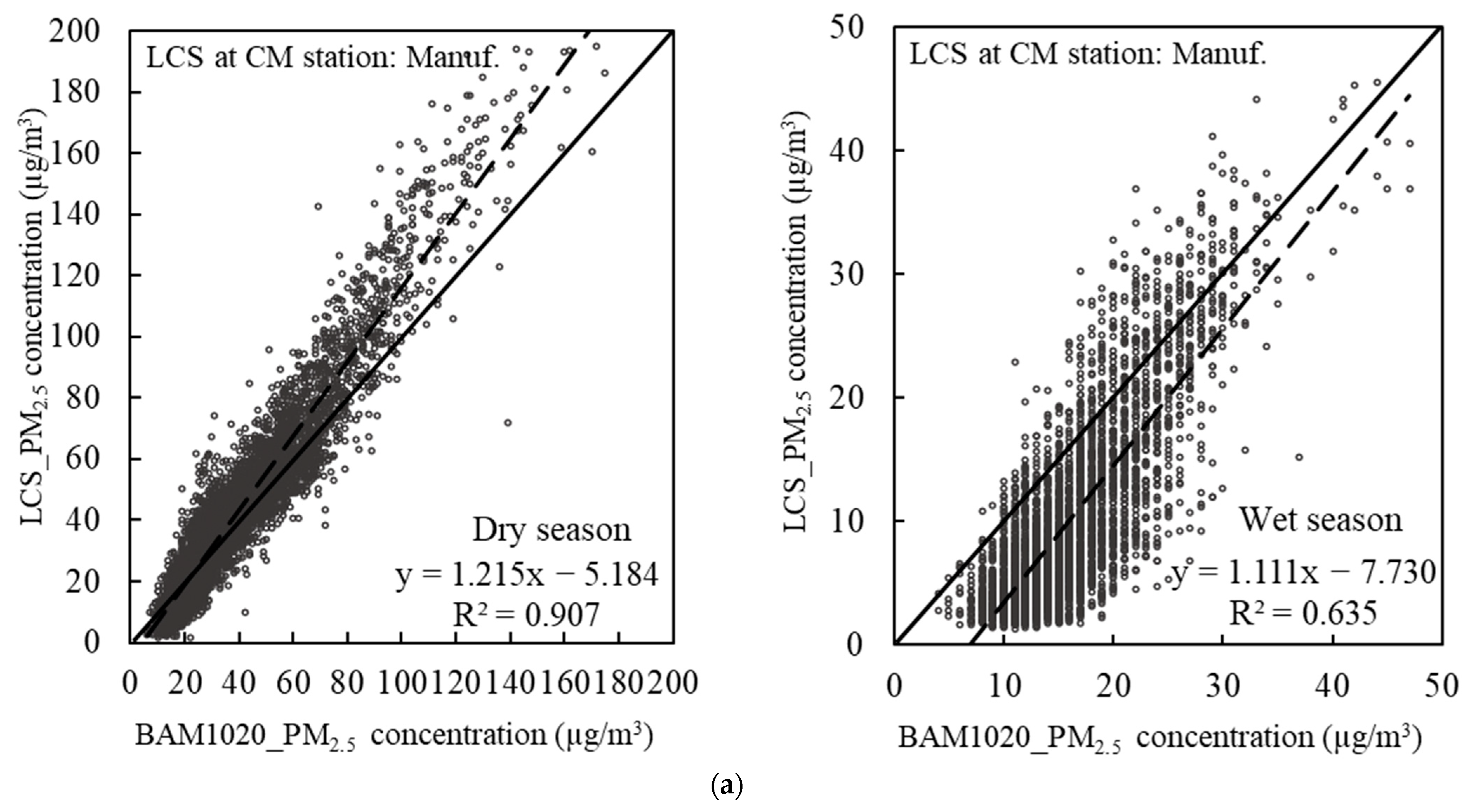
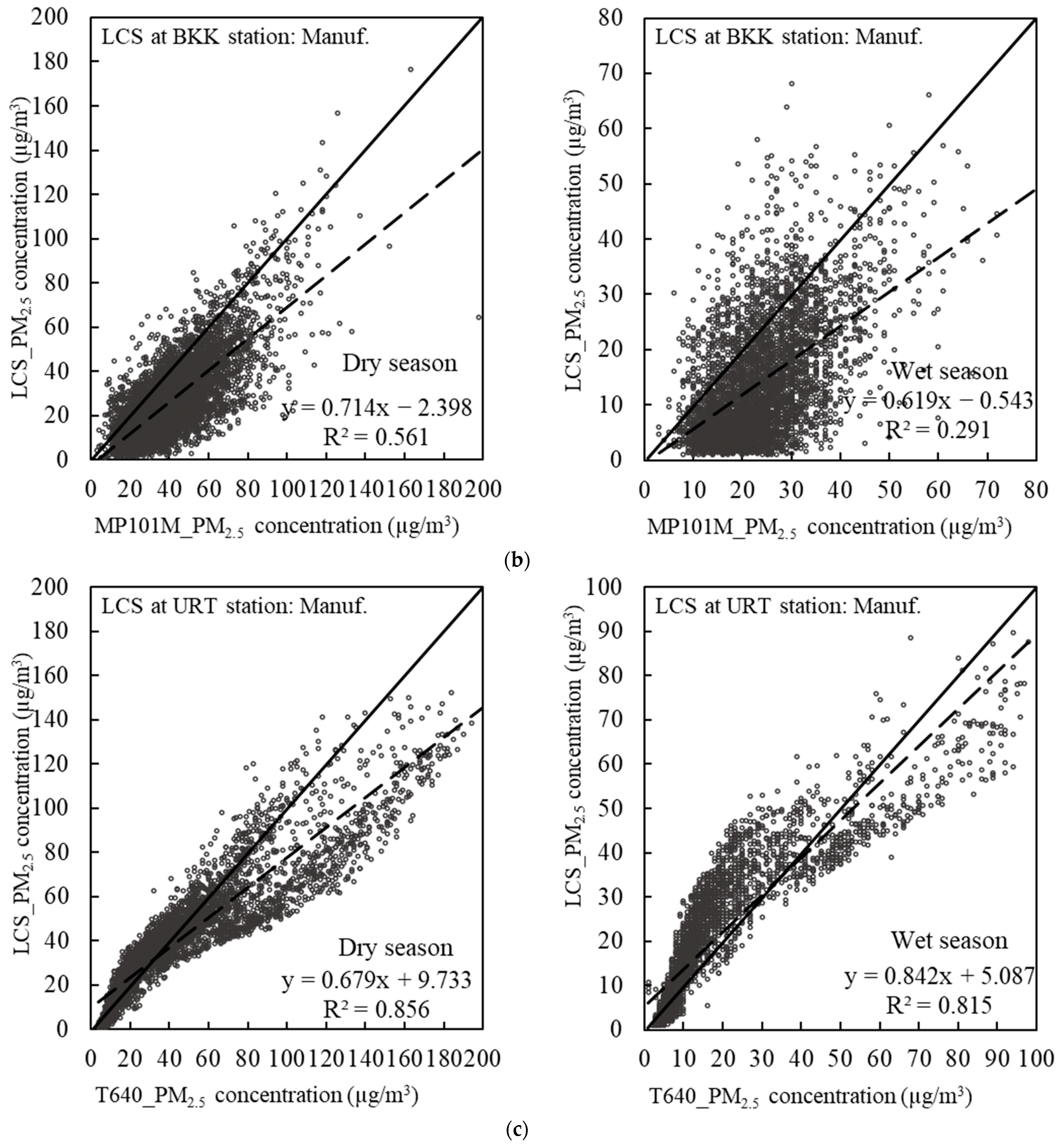
3.5. Performance Metrics for Unadjusted PM2.5 Concentration

The correlation between 1-h PM2.5 concentration from unadjusted (original) LCS and FEM measurements during the dry and wet seasons are shown in Figure 5. The values of performance metric including precision (CV), bias (slope and intercept), linearity (R2) and error (RMSE) for unadjusted LCS at each site are shown in Table 4. Reproducibility of individual LCS was assessed on the basis of CV. The mean CV for unadjusted LCS at each site during the dry (8.86 ± 7.30% to 14.47 ± 6.80%) and wet season (5.85 ± 3.86 to 12.53 ± 9.58) were at an acceptable level (CV ≤ 30%) of sensor variations. The R2 values from correlation between the unadjusted-LCS and the reference PM2.5 were acceptable at CM during the dry season with R2 = 0.907; however, during the wet season, it was poorer, with R2 = 0.635, due to larger scattering in the PM2.5 concentration at high RH level. The R2 values of LCS vs. FEM at URT during the dry (R2 = 0.856) and wet seasons (R2 = 0.815) were also acceptable with R2 > 0.7, as suggested by U.S. EPA [43]. However, at BKK, the R2 was only 0.561 during the dry season and 0.291 during the wet season. The RMSE values of unadjusted LCS vs. FEM at all sites were also higher than the values suggested by U.S. EPA [43]. Hence, the performance of PM2.5 LCS in Thailand was poor to high (R2 = 0.291–0.907) as compared with FEM instruments. This is consistent with the study of Johnson et al. [27], who reported the performance of LCS with BAM was only moderate to high (R2 = 0.35–0.81). The low performance of LCS could be attributed to the different PM emission sources, low concentration and high RH level. Before calibration, the performance of the LCS only at URT during the wet season was acceptable.

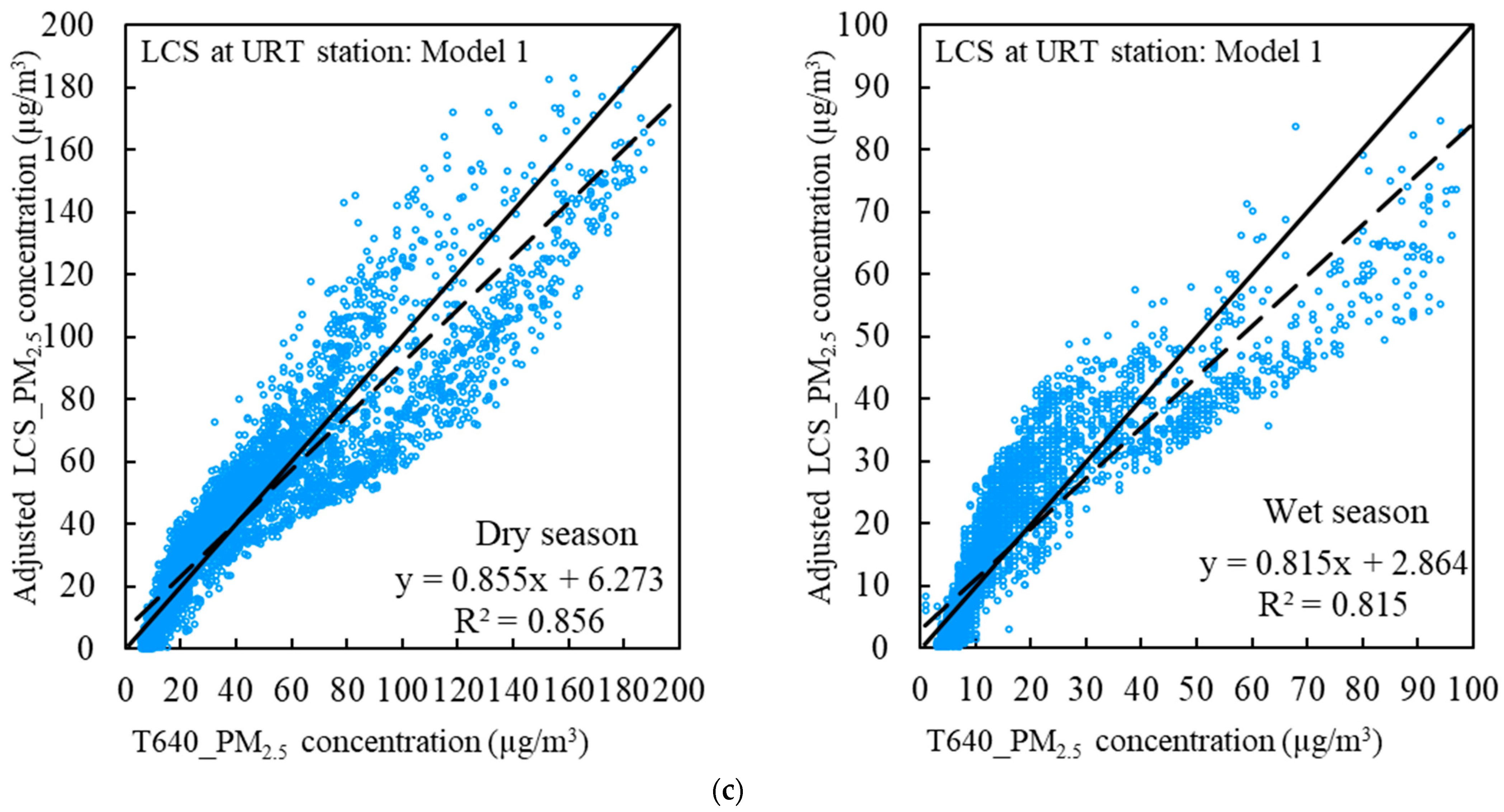
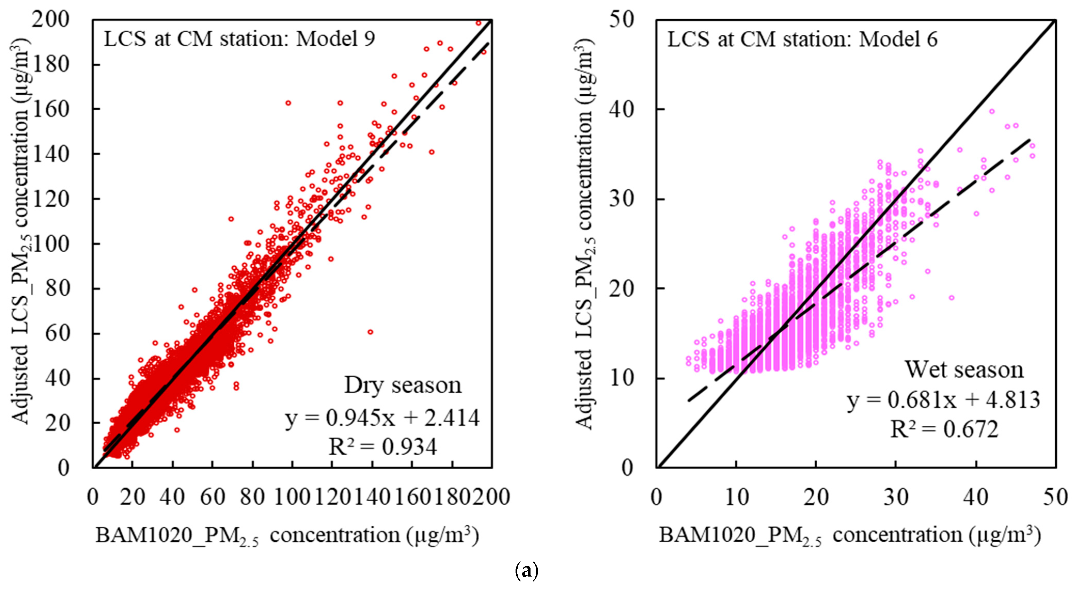
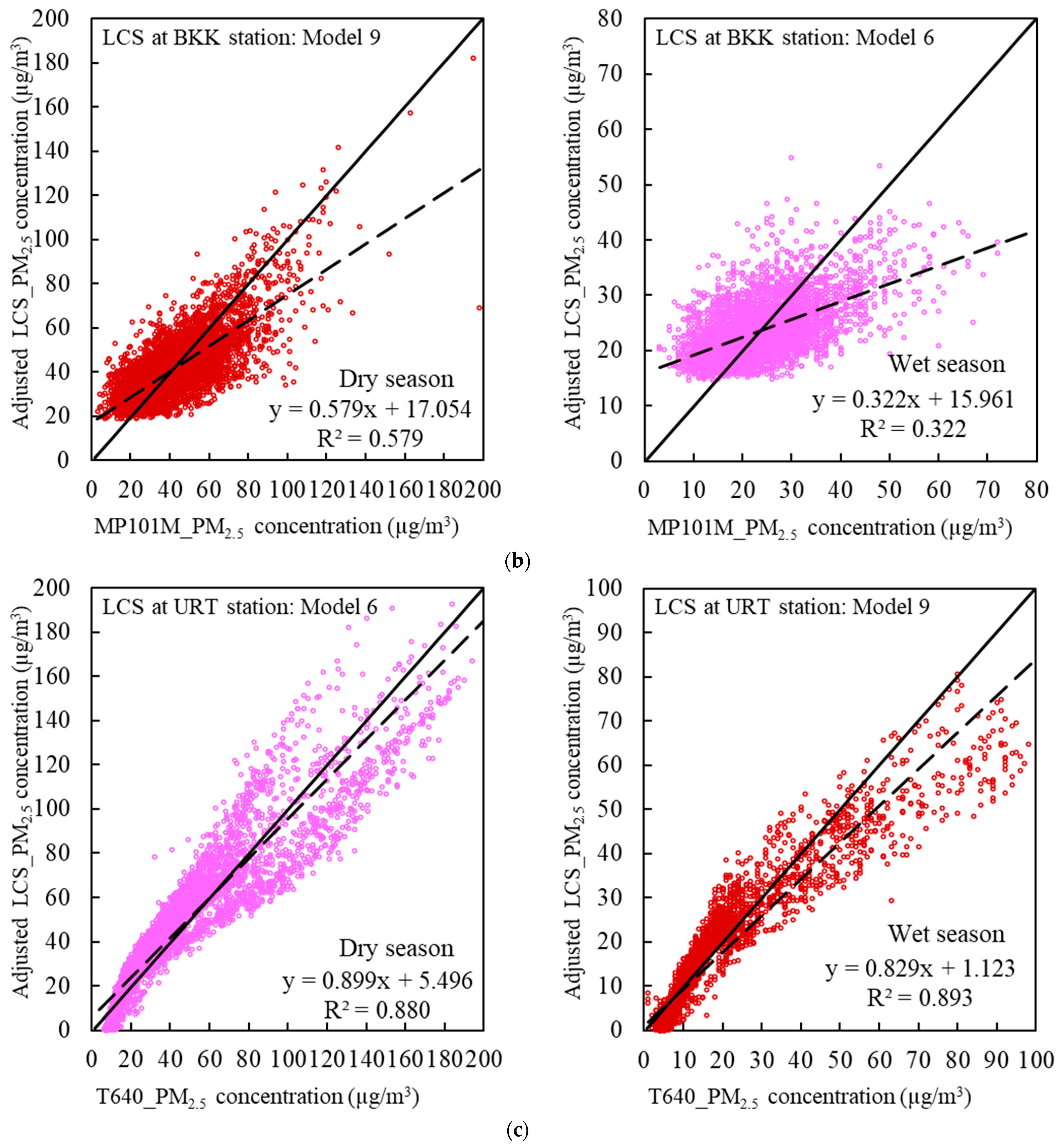
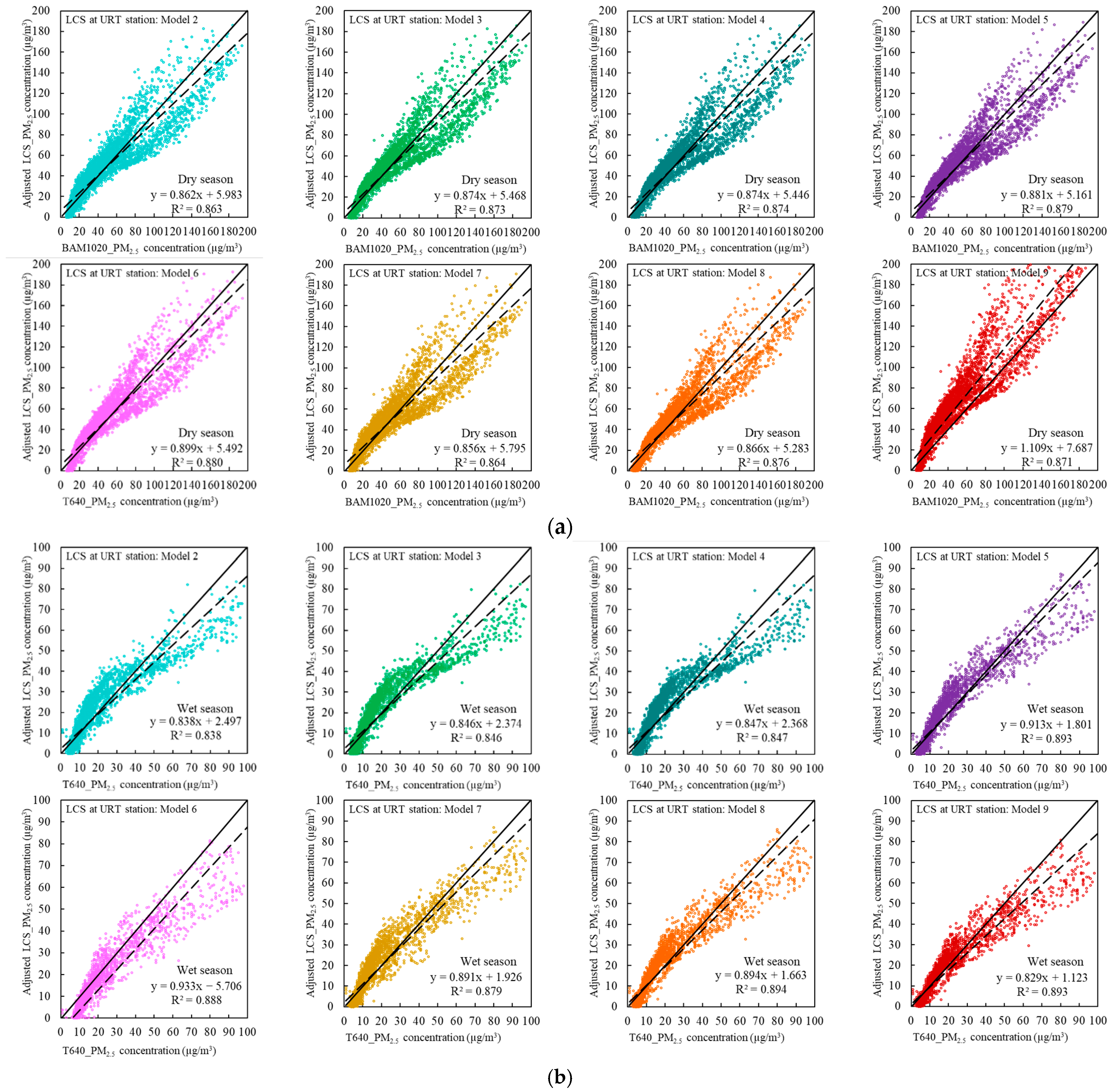
3.6. Calibration by LR Model and Performance Metrics for Adjusted LCS Based on Reference Concentration

The LR (Model 1 in Table 2) was used to calibrate 1-h PM2.5 concentrations from LCS against the reference during the dry and wet seasons. Figure 6 shows the correlation between the adjusted PM2.5 LCS by the LR model and FEM measurements at all sites for each season. The performances of the LR models are also in Table 4. After calibration by LR model, the results were improved as compared to the unadjusted PM2.5 LCS with the reduction of CV values of 42% (dry) and 46% (wet) at CM, 25% (dry) and 26% (wet) at BKK and 24% (dry) and 16% (wet) at URT. The low CV value (below 30%) was acceptable for LCS testing studies, indicating high reproducibility [43]. All CV values were well within this limit. This is consistent with Kelly et al. [26], who reported the good repeatability between Plantower sensors. Additionally, the results were significantly improved as compared to unadjusted PM2.5 from LCS with the reduced RSME values of 40.29% (dry) and 30.44% (wet) at CM, 20.83% (dry) and 20.35% (wet) at BKK and 49.15% (dry) and 12.75% (wet) at URT. However, the R2 values were not improved at all sites. This agreed with Hong et al. [21], who interpreted that the datasets were shifted to the 1:1 line without data correlation improvement.

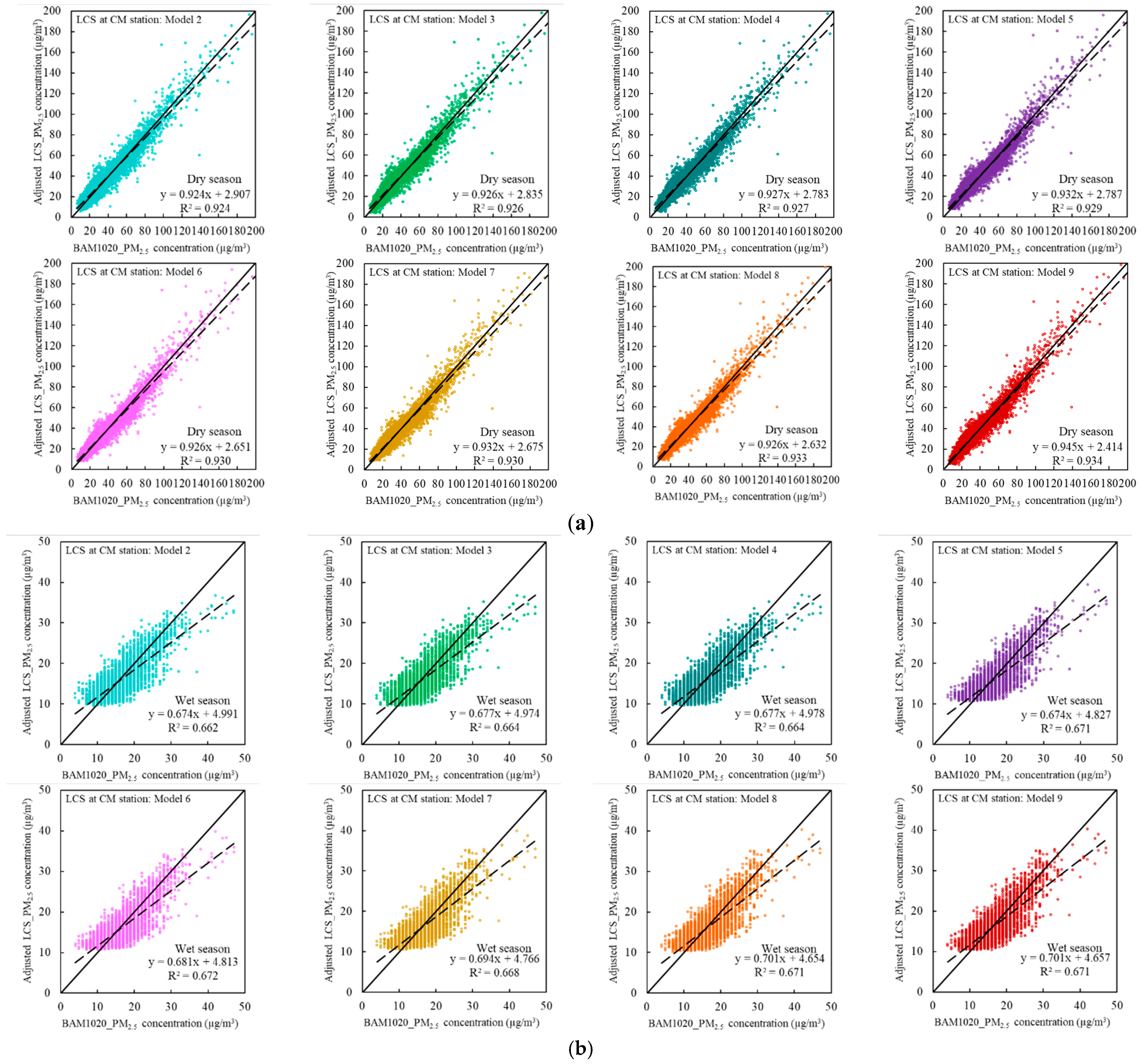
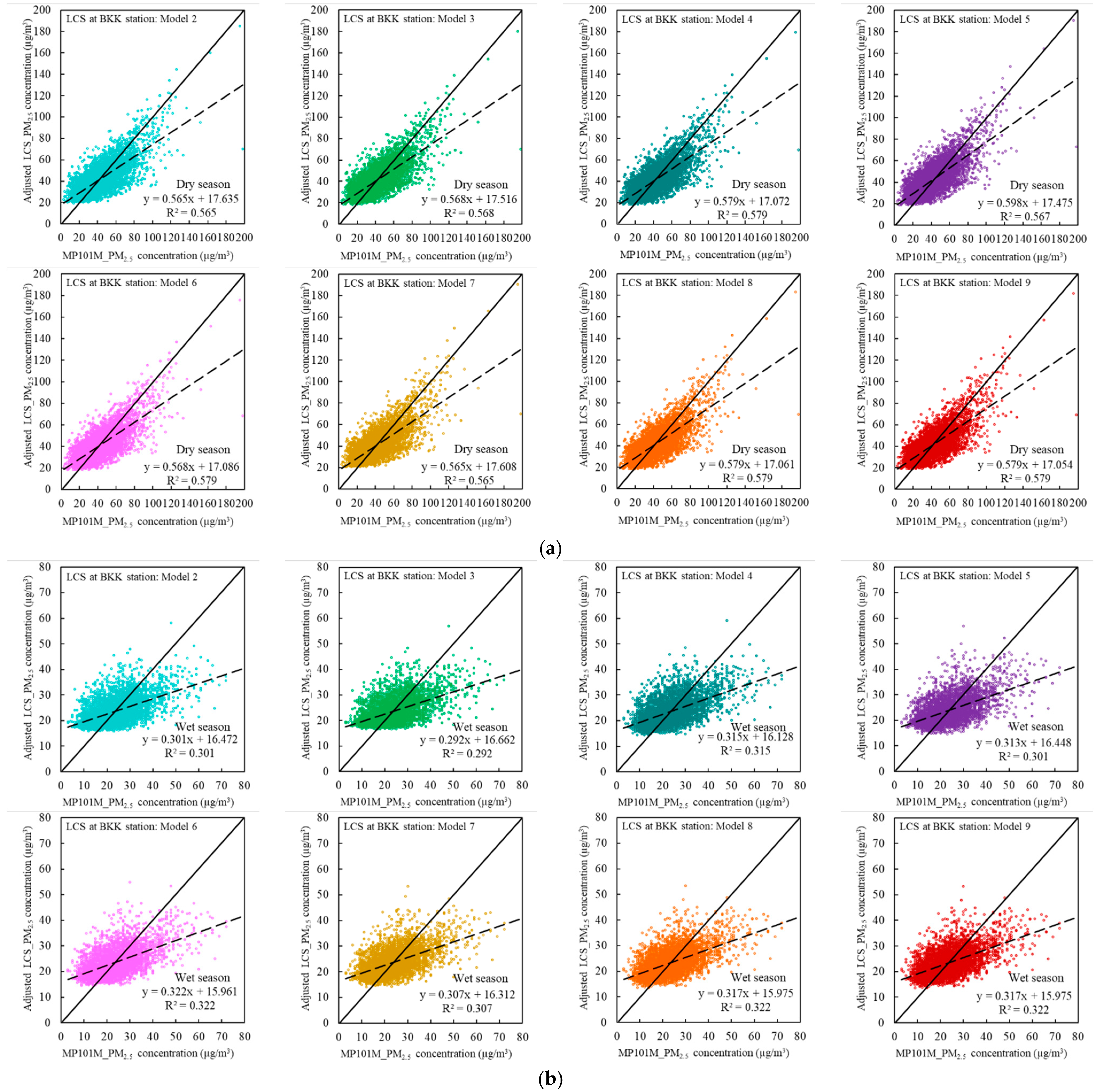
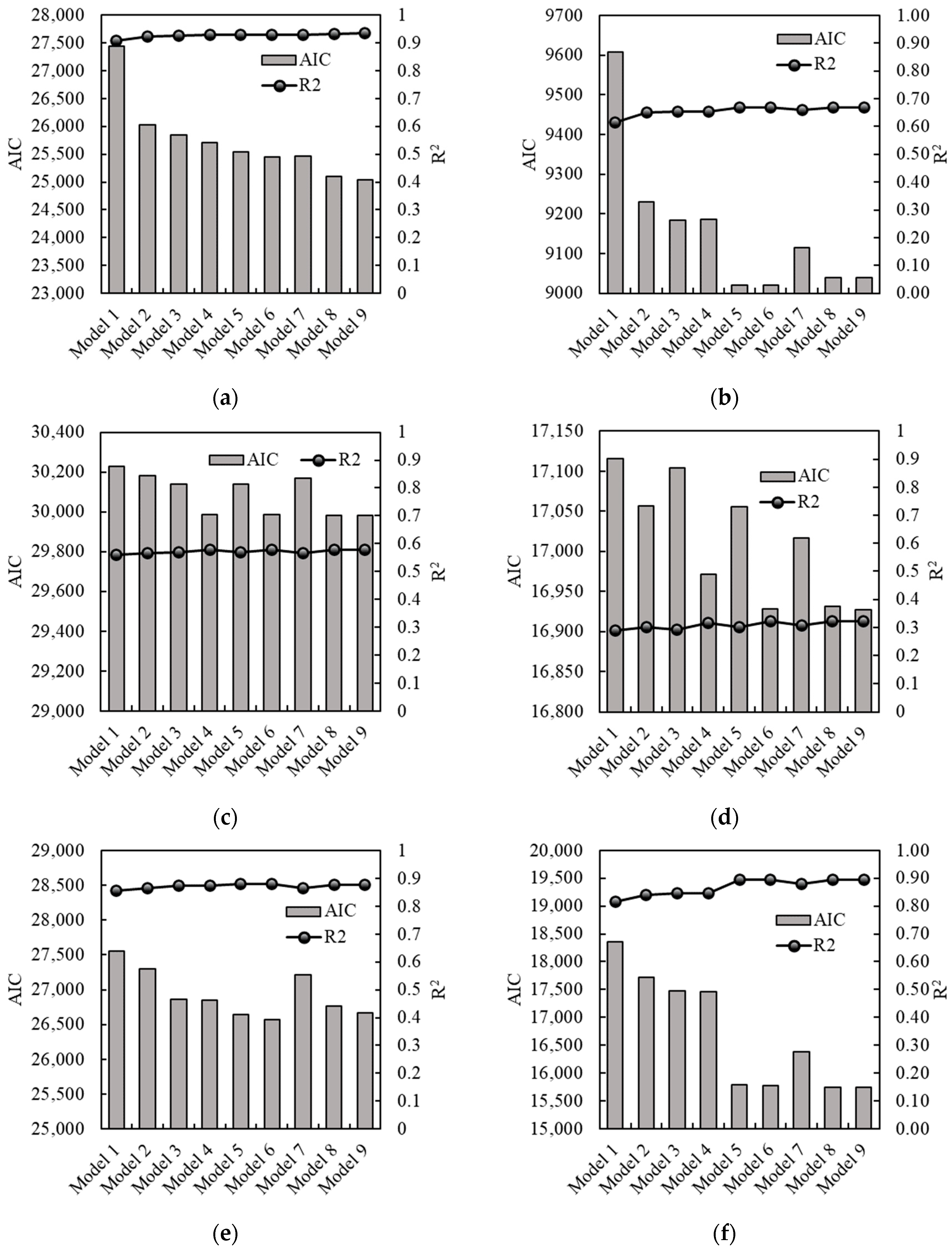
3.7. Calibration Using MLR Models to Adjust LCS Based on Reference Concentration, RH and Temperature Levels

Performance of the linear RH model (model #3) in the present study was compared with the nonlinear RH model terms [28]. The R2 for model #3 was slightly higher than the nonlinear model, as shown in Table 5. Based on this analysis, we used the linear RH model to adjust the models further.
Eight MLR models (Model#2–9 in Table 2) were used to calibrate LCS PM2.5 concentrations from LCS—see Figure A1, Figure A2 and Figure A3 in Appendix A. The correlations of the adjusted PM2.5 concentration from LCS were achieved after correction by using the MLR models based on reference concentration, RH and temperature. The best-fitted model was chosen based on lowest AIC and highest R2 (see Figure A4). The results showed that Model#6 is best for CM (wet season), BKK (wet season) and URT (dry season), while Model#9 is best for the remaining periods at each site (See Figure 7). The performance metrics of MLR model were examined only for the best fitted model at each site, as also shown in Table 4. After MLR calibration, the LCS performances were improved as compared to adjusted PM2.5 from LCS by LR model with the R2 increase of 2.98% (dry) and 5.83% (wet) at CM, 19.61% (dry) and 10.65% (wet) at BKK and 2.80% (dry) and 9.57% (wet) at URT. Additionally, the results were significantly improved as compared to the adjusted PM2.5 by LR model with the RSME reduction of 28.45% (dry) and 38.74% (wet) at CM, 20.15% (dry) and 28.81% (wet) at BKK and 48.88% (dry) and 19.86% (wet) at URT, and CV reduction of 19.15% (dry) and 15.04% (wet) at CM, 25.00% (dry) and 35.88% (wet) at BKK and 14.54% (dry) and 14.57% (wet) at URT.
The performance metrics of the LCS and FEM only at CM during the dry season and URT during the dry and wet season were acceptable with the CV: 5.76 ± 4.67–6.84 ± 4.97% (CV ≤ 30%), slope: 0.829–0.945 (slope: 1.0 ± 0.35) and intercept 1.123–5.492 µg/m3 (0 ± 5 µg/m3), R2: 0.880–0.934 (R2 ≥ 0.7) and RMSE: 4.285–5.102 µg/m3 (RMSE ≤ 7 µg/m3). The constants parameters of the best fitting calibration model at CM during the dry season and URT during both seasons are shown in Table 6. However, the correlations of the adjusted PM2.5 from LCS at BKK during both periods were not entirely consistent with the FEM values and the adjusted PM2.5 performances were not acceptable. This discrepancy might occur from variations in aerosol compositions and impacts of particle size from emission sources as described in the previous section. Moreover, The MLR model at CM during the wet season was also not suggested to use for calibration. The results showed that the FRM calibration plays more important role to the accuracy of FEM. At URT, the results showed that the LCS at URT can be calibrated during both seasons with the FEM instrument.

4. Conclusions

The effects of key factors—emission source, relative humidity, temperature and PM2.5 concentration range—on the performance of PM2.5-LCS for long periods at three different locations in Thailand during both seasons were investigated. Additionally, the calibration for LCS based on reference concentration, RH and temperature levels using LR and MLR models were also investigated to improve the performance of PM2.5-LCS in Thailand. We concluded:
  • At PM concentration < 20 µg/m3 and RH > 85%, PM2.5-LCS performance was significantly influenced.
  • Location of the PM2.5-LCS was crucial to performance: a high traffic emission area (BKK) showed low correlation with reference monitors due to the effect of small particles.
  • Unadjusted PM2.5-LCS performance varied with location, showing low to high correlations with FEM instruments (0.29 < R2 < 0.91).
  • Performances of the adjusted PM2.5-LCS at BKK in both seasons and at CM during the wet season were not acceptable due to very small particle size from emission sources, and effect of low concentrations and RH level.
  • After MRL calibration, performances of the PM2.5-LCS only at CM during the dry season and URT site during both seasons were acceptable with the CV: 5.76 ± 4.67%–6.84 ± 4.97%, slope: 0.829–0.945, intercept: 1.123–5.492 µg/m3, R2: 0.880–0.934 and RMSE: 4.285–5.102 µg/m3.
The present study showed the importance of evaluating the long-term field performance of PM2.5-LCS at different ambient conditions and locations. Calibration and validation of the PM2.5 LCS with FEM instruments in the field test is crucial to high-quality data. Moreover, understanding the key factors, including emission sources, relative humidity, temperature and PM2.5 concentration, on PM2.5-LCS performance provides crucial information for setting an achievable and reasonable guideline to enhance the quality of PM2.5-LCS data. Since the calibration of the sensors used the full dataset to develop and test the models at each station, the calibration results may differ slightly for shorter collocation periods when different dataset are used. In the future, the PM2.5-LCS performance with higher performance in low concentrations and high humidity environment are recommended.

Author Contributions

Conceptualization, R.D., T.L. and P.T.; methodology, R.D., P.T. and T.-C.L.; formal analysis, R.D. and A.S.; investigation, R.D. and A.S.; data curation, R.D.; writing—original draft preparation, R.D.; writing—review and editing, P.T., G.-Y.L., T.-C.L., C.-J.T. and J.M.; supervision, P.T. and C.-J.T.; project administration, P.T.; funding acquisition, R.D. and P.T. All authors have read and agreed to the published version of the manuscript.

Funding

This research was financially supported by the National Research Council of Thailand under the project “Standardization of Low-Cost PM2.5 Sensors from Research” and Prince of Songkla University and Ministry of Higher Education, Science, Research and Innovation under the Reinventing University Project, and the 2022 SATU-PSU JRS project grant (grant No. 1/2565).

Institutional Review Board Statement

Not applicable.

Informed Consent Statement

Not applicable.

Data Availability Statement

The data presented in this study are available on request from the corresponding author.

Acknowledgments

Data were supplied by the Pollution Control Department, Thailand. We also thank the Digital Research and Innovation Institute, Prince of Songkla University, who supported the LCS instruments and supplied the data.

Conflicts of Interest

The authors declare no conflict of interest.

Appendix A

Appendix A.1

Figure A1. Correlation of 1-h PM2.5 concentration between adjusted LCS by MRL models vs. FEM during the (a) dry and (b) wet seasons at CM. The solid line is the line with slope =1 while the dashed line represents the fitting.
Atmosphere 14 00496 g0a1

Appendix A.2

Figure A2. Correlation of 1-h PM2.5 concentration between adjusted LCS by MRL models vs. FEM during the (a) dry and (b) wet seasons at BKK. The solid line is the line with slope =1 while the dashed line represents the fitting.
Atmosphere 14 00496 g0a2

Appendix A.3

Figure A3. Correlation of 1-h PM2.5 concentration between adjusted LCS by MRL models vs. FEM during the (a) dry and (b) wet seasons. The solid line is the line with slope =1 while the dashed line represents the fitting.
Atmosphere 14 00496 g0a3

Appendix A.4

Figure A4. AIC and R2 values of LR and MLR calibration models during the (a) dry and (b) wet seasons at CM, (c) dry and (d) wet seasons at BKK and (e) dry and (f) wet seasons at URT.
Atmosphere 14 00496 g0a4

References

  1. Pani, S.K.; Chantara, S.; Khamkaew, C.; Lee, C.T.; Lin, N.H. Biomass burning in the northern peninsular Southeast Asia: Aerosol chemical profile and potential exposure. Atmos. Res. 2019, 224, 180–195. [Google Scholar] [CrossRef] [Green Version]
  2. Chantara, S.; Thepnuan, D.; Wiriya, W.; Prawan, S.; Tsai, Y.I. Emissions of pollutant gases, fine particulate matters and their significant tracers from biomass burning in an open-system combustion chamber. Chemosphere 2019, 224, 407–416. [Google Scholar] [CrossRef] [PubMed]
  3. Thepnuan, D.; Chantara, S.; Lee, C.T.; Lin, N.H.; Tsai, Y.I. Molecular markers for biomass burning associated with the characterization of PM2.5 and component sources during dry season haze episodes in Upper South East Asia. Sci. Total Environ. 2019, 658, 708–722. [Google Scholar] [CrossRef] [PubMed]
  4. Chomanee, J.; Thongboon, K.; Tekasakul, S.; Furuuchi, M.; Dejchanchaiwong, R.; Tekasakul, P. Physicochemical and toxicological characteristics of nanoparticles in aerosols in southern Thailand during recent haze episodes in lower southeast Asia. J. Environ. Sci. 2020, 94, 72–80. [Google Scholar] [CrossRef] [PubMed]
  5. ChooChuay, C.; Pongpiachan, S.; Tipmanee, D.; Deelaman, W.; Suttinun, O.; Wang, Q.; Xing, L.; Li, G.; Han, Y.; Palakun, J.; et al. Long-range Transboundary Atmospheric Transport of Polycyclic Aromatic Hydrocarbons, Carbonaceous Compositions, and Water-soluble Ionic Species in Southern Thailand. Aerosol. Air Qual. Res. 2020, 20, 1591–1606. [Google Scholar] [CrossRef]
  6. Dejchanchaiwong, R.; Tekasakul, P.; Tekasakul, S.; Phairuang, W.; Nim, N.; Sresawasd, C.; Thongboon, K.; Thongyen, T.; Suwattiga, P. Impact of transport of fine and ultrafine particles from open biomass burning on air quality during 2019 Bangkok haze episode. J. Environ. Sci. 2020, 97, 149–161. [Google Scholar] [CrossRef]
  7. Boongla, Y.; Chanonmuang, P.; Hata, M.; Furuuchi, M.; Phairuang, W. The characteristics of carbonaceous particles down to the nanoparticle range in Rangsit city in the Bangkok Metropolitan Region, Thailand. Environ. Pollut. 2021, 272, 115940. [Google Scholar] [CrossRef]
  8. Dejchanchaiwong, R.; Tekasakul, P. Effects of Coronavirus Induced City Lockdown on PM2.5 and Gaseous Pollutant Concentrations in Bangkok. Aerosol. Air Qual. Res. 2021, 21, 200418. [Google Scholar] [CrossRef]
  9. Sresawasd, C.; Chetiyanukornkul, T.; Suriyawong, P.; Tekasakul, S.; Furuuchi, M.; Hata, M.; Malinee, R.; Tekasakul, P.; Dejchanchaiwong, R. Influence of Meteorological Conditions and Fire Hotspots on PM0.1 in Northern Thailand during Strong Haze Episodes and Carbonaceous Aerosol Characterization. Aerosol. Air Qual. Res. 2021, 21, 210069. [Google Scholar] [CrossRef]
  10. ChooChuay, C.; Pongpiachan, S.; Tipmanee, D.; Deelaman, W.; Iadtem, N.; Suttinun, O.; Wang, Q.; Xing, L.; Li, G.; Han, Y.; et al. Effects of Agricultural Waste Burning on PM2.5-Bound Polycyclic Aromatic Hydrocarbons, Carbonaceous Compositions, and Water-Soluble Ionic Species in the Ambient Air of Chiang-Mai, Thailand. Polycycl. Aromat. Compd. 2022, 42, 749–770. [Google Scholar] [CrossRef]
  11. Mahasakpan, N.; Chaisongkaew, P.; Inerb, M.; Nim, N.; Phairuang, W.; Tekasakul, S.; Furuuchi, M.; Hata, M.; Kaosol, T.; Tekasakul, P.; et al. Fine and ultrafine particle- and gas-polycyclic aromatic hydrocarbons affecting southern Thailand air quality during transboundary haze and potential health effects. J. Environ. Sci. 2023, 124, 253–267. [Google Scholar] [CrossRef] [PubMed]
  12. Kim Oanh, N.T.; Permadi, D.A.; Hopke, P.K.; Smith, K.R.; Dong, N.P.; Dang, A.N. Annual emissions of air toxics emitted from crop residue open burning in Southeast Asia over the period of 2010–2015. Atmos. Environ. 2018, 187, 163–173. [Google Scholar] [CrossRef]
  13. GISTDA. Thailand Fire Monitoring System. Available online: https://fire.gistda.or.th/ (accessed on 9 November 2022).
  14. Office of Agricultural Economics. Agricultural Production during the Year 2016-2019. Available online: https://www.oae.go.th/view/1/ (accessed on 4 November 2022).
  15. Oanh, N.T.K.; Ly, B.T.; Tipayarom, D.; Manandhar, B.R.; Prapat, P.; Simpson, C.D.; Liu, L.J.S. Characterization of particulate matter emission from open burning of rice straw. Atmos. Environ. 2011, 45, 493–502. [Google Scholar] [CrossRef] [Green Version]
  16. PCD. Thailand’s Air Quality and Situation Reports. Available online: http://air4thai.pcd.go.th/webV2/history/ (accessed on 15 November 2022).
  17. U.S.EPA. List of Designated Reference and Equivalent Methods; U.S. Environmental Protection Agency: Washington, DC, USA, 2017.
  18. Hu, J.; Zhang, H.; Chen, S.H.; Wiedinmyer, C.; Vandenberghe, F.; Ying, Q.; Kleeman, M.J. Predicting Primary PM 2.5 and PM 0.1 Trace Composition for Epidemiological Studies in California. Environ. Sci. Technol. 2014, 48, 4971–4979. [Google Scholar] [CrossRef]
  19. Bai, L.; Huang, L.; Wang, Z.; Ying, Q.; Zheng, J.; Shi, X.; Hu, J. Long-term field Evaluation of Low-cost Particulate Matter Sensors in Nanjing. Aerosol Air Qual. Res. 2020, 20, 242–253. [Google Scholar] [CrossRef]
  20. Liu, X.; Jayaratne, R.; Thai, P.; Kuhn, T.; Zing, I.; Christensen, B.; Lamont, R.; Dunbabin, M.; Zhu, S.; Gao, J.; et al. Low-cost sensors as an alternative for long-term air quality monitoring. Environ. Res. 2020, 185, 109438. [Google Scholar] [CrossRef]
  21. Hong, G.-H.; Le, T.-C.; Tu, J.-W.; Wang, C.; Chang, S.-C.; Yu, J.-Y.; Lin, G.-Y.; Aggarwal, S.G.; Tsai, C.-J. Long-term evaluation and calibration of three types of low-cost PM2.5 sensors at different air quality monitoring stations. J. Aerosol Sci. 2021, 157, 105829. [Google Scholar] [CrossRef]
  22. Air Quality Information Center. Air Pollution in Thailand. Available online: https://pm2_5.nrct.go.th/ (accessed on 1 November 2022).
  23. Barkjohn, K.K.; Holder, A.L.; Frederick, S.G.; Clements, A.L. Correction and Accuracy of PurpleAir PM2.5 Measurements for Extreme Wildfire Smoke. Sensors 2022, 22, 9669. [Google Scholar] [CrossRef]
  24. Chu, H.J.; Ali, M.Z.; He, Y.C. Spatial calibration and PM2.5 mapping of low-cost air quality sensors. Sci. Rep. 2020, 10, 22079. [Google Scholar] [CrossRef]
  25. Tagle, M.; Rojas, F.; Reyes, F.; Vásquez, Y.; Hallgren, F.; Lindén, J.; Kolev, D.; Watne, Å.K.; Oyola, P. Field performance of a low-cost sensor in the monitoring of particulate matter in Santiago, Chile. Environ. Monit. Assess. 2020, 192, 171. [Google Scholar] [CrossRef] [Green Version]
  26. Kelly, K.; Whitaker, J.; Petty, A.; Widmer, C.; Dybwad, A.; Sleeth, D.; Martin, R.; Butterfield, A. Ambient and laboratory evaluation of a low-cost particulate matter sensor. Environ. Pollut. 2017, 221, 491–500. [Google Scholar] [CrossRef] [PubMed]
  27. Johnson, K.K.; Bergin, M.H.; Russell, A.G.; Hagler, G.S.W. Field Test of Several Low-Cost Particulate Matter Sensors in High and Low Concentration Urban Environments. Aerosol Air Qual. Res. 2018, 18, 565–578. [Google Scholar] [CrossRef]
  28. Zheng, T.; Bergin, M.H.; Johnson, K.K.; Tripathi, S.N.; Shirodkar, S.; Landis, M.S.; Sutaria, R.; Carlson, D.E. Field evaluation of low-cost particulate matter sensors in high- and low-concentration environments. Atmos. Meas. Tech. 2018, 11, 4823–4846. [Google Scholar] [CrossRef] [Green Version]
  29. Kosmopoulos, G.; Salamalikis, V.; Pandis, S.N.; Yannopoulos, P.; Bloutsos, A.A.; Kazantzidis, A. Low-cost sensors for measuring airborne particulate matter: Field evaluation and calibration at a South-Eastern European site. Sci. Total Environ. 2020, 748, 141396. [Google Scholar] [CrossRef] [PubMed]
  30. Castell, N.; Dauge, F.R.; Schneider, P.; Vogt, M.; Lerner, U.; Fishbain, B.; Broday, D.; Bartonova, A. Can commercial low-cost sensor platforms contribute to air quality monitoring and exposure estimates? Environ. Int. 2017, 99, 293–302. [Google Scholar] [CrossRef] [PubMed]
  31. Zusman, M.; Schumacher, C.S.; Gassett, A.J.; Spalt, E.W.; Austin, E.; Larson, T.V.; Carvlin, G.; Seto, E.; Kaufman, J.D.; Sheppard, L. Calibration of low-cost particulate matter sensors: Model development for a multi-city epidemiological study. Environ. Int. 2020, 134, 105329. [Google Scholar] [CrossRef]
  32. Levy Zamora, M.; Xiong, F.; Gentner, D.; Kerkez, B.; Kohrman-Glaser, J.; Koehler, K. Field and Laboratory Evaluations of the Low-Cost Plantower Particulate Matter Sensor. Environ. Sci. Technol. 2019, 53, 838–849. [Google Scholar] [CrossRef]
  33. Jayarathne, T.; Stockwell, C.E.; Gilbert, A.A.; Daugherty, K.; Cochrane, M.A.; Ryan, K.C.; Putra, E.I.; Saharjo, B.H.; Nurhayati, A.D.; Albar, I.; et al. Chemical characterization of fine particulate matter emitted by peat fires in Central Kalimantan, Indonesia, during the 2015 El Niño. Atmos. Chem. Phys. 2018, 18, 2585–2600. [Google Scholar] [CrossRef] [Green Version]
  34. Giordano, M.R.; Malings, C.; Pandis, S.N.; Presto, A.A.; McNeill, V.; Westervelt, D.M.; Beekmann, M.; Subramanian, R. From low-cost sensors to high-quality data: A summary of challenges and best practices for effectively calibrating low-cost particulate matter mass sensors. J. Aerosol Sci. 2021, 158, 105833. [Google Scholar] [CrossRef]
  35. Liang, L. Calibrating low-cost sensors for ambient air monitoring: Techniques, trends, and challenges. Environ. Res. 2021, 197, 111163. [Google Scholar] [CrossRef]
  36. Park, D.; Yoo, G.W.; Park, S.H.; Lee, J.H. Assessment and Calibration of a Low-Cost PM2.5 Sensor Using Machine Learning (HybridLSTM Neural Network): Feasibility Study to Build an Air Quality Monitoring System. Atmosphere 2021, 12, 1306. [Google Scholar] [CrossRef]
  37. Barkjohn, K.K.; Gantt, B.; Clements, A.L. Development and application of a United States-wide correction for PM&lt;sub&gt;2.5&lt;/sub&gt; data collected with the PurpleAir sensor. Atmos. Meas. Tech. 2021, 14, 4617–4637. [Google Scholar] [CrossRef] [PubMed]
  38. Kim, S.; Park, S.; Lee, J. Evaluation of Performance of Inexpensive Laser Based PM2.5 Sensor Monitors for Typical Indoor and Outdoor Hotspots of South Korea. Appl. Sci. 2019, 9, 1947. [Google Scholar] [CrossRef] [Green Version]
  39. Zhou, Y. Digital Universal Particle Concentration Sensor pms7003 Series Data Manual. Available online: https://download.kamami.pl/p564008-PMS7003%20series%20data%20manua_English_V2.5.pdf (accessed on 9 November 2022).
  40. Jiang, Y.; Zhu, X.; Chen, C.; Ge, Y.; Wang, W.; Zhao, Z.; Cai, J.; Kan, H. On-field test and data calibration of a low-cost sensor for fine particles exposure assessment. Ecotoxicol. Environ. Saf. 2021, 211, 111958. [Google Scholar] [CrossRef] [PubMed]
  41. Zhou, Y. Digital Universal Particle Concentration Sensor pms5003 Series Data Manual. Available online: https://www.aqmd.gov/docs/default-source/aq-spec/resources-page/plantower-pms5003-manual_v2-3.pdf (accessed on 9 November 2022).
  42. Bulot, F.M.; Johnston, S.J.; Basford, P.J.; Easton, N.H.; Apetroaie-Cristea, M.; Foster, G.L.; Morris, A.K.; Cox, S.J.; Loxham, M. Long-term field comparison of multiple low-cost particulate matter sensors in an outdoor urban environment. Sci. Rep. 2019, 9, 7497. [Google Scholar] [CrossRef] [Green Version]
  43. U.S.EPA. Performance Testing Protocols, Metrics, and Target Values for Fine Particulate Matter Air Sensor; U.S. Environmental Protection Agency: Washington, DC, USA, 2021.
  44. Adam, M.G.; Tran, P.T.M.; Bolan, N.; Balasubramanian, R. Biomass burning-derived airborne particulate matter in Southeast Asia: A critical review. J. Hazard. Mater. 2021, 407, 124760. [Google Scholar] [CrossRef]
  45. TMD. Monthly Mean Rainfall in Thailand (mm) 30 Years. Available online: https://www.tmd.go.th/en/ClimateChart/monthly-mean-rainfall-in-thailand-mm-30-years (accessed on 1 November 2022).
  46. Land Development Department. Land Use and Land Cover in 2019. Available online: https://www.ldd.go.th/home/ (accessed on 9 November 2022).
  47. Boonman, T.; Garivait, S.; Bonnet, S.; Junpen, A. An Inventory of Air Pollutant Emissions from Biomass Open Burning in Thailand Using MODIS Burned Area Product (MCD45A1). J. Sustain. Energy Environ. 2014, 5, 85–94. [Google Scholar]
  48. Oanh, N.T.K.; Tipayarom, A.; Bich, T.L.; Tipayarom, D.; Simpson, C.D.; Hardie, D.; Liu, L.J.S. Characterization of gaseous and semi-volatile organic compounds emitted from field burning of rice straw. Atmos. Environ. 2015, 119, 182–191. [Google Scholar] [CrossRef]
  49. Hagler, G.; Hanley, T.; Hassett-Sipple, B.; Vanderpool, R.; Smith, M.; Wilbur, J.; Wilbur, T.; Oliver, T.; Shand, D.; Vidacek, V.; et al. Evaluation of two collocated federal equivalent method PM2.5 instruments over a wide range of concentrations in Sarajevo, Bosnia and Herzegovina. Atmos. Pollut. Res. 2022, 13, 101374. [Google Scholar] [CrossRef]
  50. Wang, J.; Ogawa, S. Effects of Meteorological Conditions on PM2.5 Concentrations in Nagasaki, Japan. Int. J. Environ. Res. Public Health 2015, 12, 9089–9101. [Google Scholar] [CrossRef]
  51. Liu, X.; Zhang, Y.-L.; Peng, Y.; Xu, L.; Zhu, C.; Cao, F.; Zhai, X.; Haque, M.M.; Yang, C.; Chang, Y.; et al. Chemical and optical properties of carbonaceous aerosols in Nanjing, eastern China: Regionally transported biomass burning contribution. Atmos. Chem. Phys. 2019, 19, 11213–11233. [Google Scholar] [CrossRef] [Green Version]
  52. Li, J.; Mattewal, S.K.; Patel, S.; Biswas, P. Evaluation of Nine Low-cost-sensor-based Particulate Matter Monitors. Aerosol Air Qual. Res. 2020, 20, 254–270. [Google Scholar] [CrossRef] [Green Version]
  53. Badura, M.; Batog, P.; Drzeniecka-Osiadacz, A.; Modzel, P. Evaluation of Low-Cost Sensors for Ambient PM2.5 Monitoring. J. Sens. 2018, 2018, 5096540. [Google Scholar] [CrossRef] [Green Version]
  54. Zou, Y.; Clark, J.D.; May, A.A. A systematic investigation on the effects of temperature and relative humidity on the performance of eight low-cost particle sensors and devices. J. Aerosol Sci. 2021, 152, 105715. [Google Scholar] [CrossRef]
  55. Liu, H.Y.; Schneider, P.; Haugen, R.; Vogt, M. Performance Assessment of a Low-Cost PM2.5 Sensor for a near Four-Month Period in Oslo, Norway. Atmosphere 2019, 10, 41. [Google Scholar] [CrossRef] [Green Version]
  56. Malings, C.; Tanzer, R.; Hauryliuk, A.; Kumar, S.P.N.; Zimmerman, N.; Kara, L.B.; Presto, A.A.; Subramanian, R. Development of a general calibration model and long-term performance evaluation of low-cost sensors for air pollutant gas monitoring. Atmos. Meas. Tech. 2019, 12, 903–920. [Google Scholar] [CrossRef] [Green Version]
  57. Magi, B.I.; Cupini, C.; Francis, J.; Green, M.; Hauser, C. Evaluation of PM2.5 measured in an urban setting using a low-cost optical particle counter and a Federal Equivalent Method Beta Attenuation Monitor. Aerosol Sci. Technol. 2020, 54, 147–159. [Google Scholar] [CrossRef]
  58. Chang, C.T.; Tsai, C.J. A model for the relative humidity effect on the readings of the PM10 beta-gauge monitor. J. Aerosol Sci. 2003, 34, 1685–1697. [Google Scholar] [CrossRef]
  59. Takahashi, K.; Minoura, H.; Sakamoto, K. Examination of discrepancies between beta-attenuation and gravimetric methods for the monitoring of particulate matter. Atmos. Environ. 2008, 42, 5232–5240. [Google Scholar] [CrossRef]
  60. Kiss, G.; Imre, K.; Molnár, Á.; Gelencsér, A. Bias caused by water adsorption in hourly PM measurements. Atmos. Meas. Tech 2017, 10, 2477–2484. [Google Scholar] [CrossRef] [Green Version]
  61. Wu, Z.; Hu, M.; Lin, P.; Liu, S.; Wehner, B.; Wiedensohler, A. Particle number size distribution in the urban atmosphere of Beijing, China. Atmos. Environ. 2008, 42, 7967–7980. [Google Scholar] [CrossRef]
  62. Samae, H.; Tekasakul, S.; Tekasakul, P.; Furuuchi, M. Emission factors of ultrafine particulate matter (PM < 0.1 μm) and particle-bound polycyclic aromatic hydrocarbons from biomass combustion for source apportionment. Chemosphere 2021, 262, 127846. [Google Scholar]
  63. Hata, M.; Chomanee, J.; Thongyen, T.; Bao, L.; Tekasakul, S.; Tekasakul, P.; Otani, Y.; Furuuchi, M. Characteristics of nanoparticles emitted from burning of biomass fuels. J. Environ. Sci. 2014, 26, 1913–1920. [Google Scholar] [CrossRef] [PubMed]
  64. Kuula, J.; Friman, M.; Helin, A.; Niemi, J.V.; Aurela, M.; Timonen, H.; Saarikoski, S. Utilization of scattering and absorption-based particulate matter sensors in the environment impacted by residential wood combustion. J. Aerosol Sci. 2020, 150, 105671. [Google Scholar] [CrossRef]
Figure 1. (a) Custom designed printed circuit board and its components for the Plantower PMS7003 sensor package; (b) closed louver box housing all components for outdoor monitoring.
Atmosphere 14 00496 g001
Figure 2. Sampling locations.
Atmosphere 14 00496 g002
Figure 3. Time series of 1-h PM2.5 concentrations from LCS and FEM; ratio of LCS to FEM, RH and temperature at (a) CM, (b) BKK and (c) URT: the red line indicates the ratio LCS/FEM = 1.
Atmosphere 14 00496 g003aAtmosphere 14 00496 g003b
Figure 4. Distribution of relative error of PM2.5 mass concentrations measured by LCS and FEM vs. FEM and relative error vs. RH&T at (a) CM (b) BKK and (c) URT. Note: a different FEM was used at each sampling station.
Atmosphere 14 00496 g004
Figure 5. Comparison between 1-h PM2.5 concentration between unadjusted LCS vs. FEM during the dry and wet seasons at (a) CM, (b) BKK and (c) URT. The solid line is the line with slope =1 while the dashed line represents the fitting.
Atmosphere 14 00496 g005aAtmosphere 14 00496 g005b
Figure 6. Correlation between LCS LR models and FEM values for 1-h PM2.5 concentration during the dry and wet seasons at (a) CM, (b) BKK and (c) URT. The solid line is the line with slope =1 while the dashed line represents the fitting.
Atmosphere 14 00496 g006aAtmosphere 14 00496 g006b
Figure 7. Correlation between LCS and FEM 1-h PM2.5 concentrations using MRL models during both seasons at (a) CM, (b) BKK and (c) URT—model 6: pink scatters, model 9: red points. The solid line is the line with slope =1 while the dashed line represents the fitting.
Atmosphere 14 00496 g007aAtmosphere 14 00496 g007b
Table 1. Sampling locations, periods, and FEM instruments at three monitoring stations.
RegionsStation NameLocationsInstruments
(U.S. EPA FEM Approved)
Measurement TechniqueDurationDry SeasonWet Season
Northern Thailand: Chiang Mai (CM site)Chiang Mai municipal center
(PCD station #35)
Lat:18.83737, Lon:98.97132BAM1020, MetOne, USA Beta attenuation 1 Dec 2020–31 Mar 2022
(16 months)
Dec 2020–Apr 2021 & Nov 2021–Mar 2022 (n = 7043)May–Oct 2021
(n = 4005)
Central Thailand:
Bangkok (BKK site)
National Housing Authority Public Community Din Daeng
(PCD station#54)
Lat:13.76470,
Lon:100.55195
MP101M, ENVEA, FranceBeta attenuation 1 Jan 2021–31 Mar 2022
(15 months)
Jan 2021–Apr 2021 & Nov 2021–Mar 2022
(n = 6022)
May–Oct 2021
(n = 4042)
Northeast Thailand:
Ubon Ratchathani (URT site)
Ubon Ratchathani Provincial Administrative Organization
(PCD station#83)
Lat:15.245169, Lon:104.84680T640, Teledyne, USA Light Scattering1 Mar 2020–31 May 2021
(15 months)
Mar–Apr 2020 & Nov 2020–Mar 2021
(n = 5198)
May–Oct 2020 & May 2021
(n = 4671)
Table 2. Developed calibration models by LR and MLR to improve LCS accuracy.
#ModelTypeEquations
1LR PM 2.5 - FEM = a 1 + a 2 Raw   PM 2.5 - LCS
2MLR PM 2.5 - FEM =   b 1 + b 2 Raw   PM 2.5 - LCS + b 3 T
3MLR PM 2.5 - FEM = c 1 + c 2 Raw   PM 2.5 - LCS + c 3 R H
4MLR PM 2.5 - FEM = d 1 + d 2 Raw   PM 2.5 - LCS + d 3 T + d 4 R H
5MLR PM 2.5 - FEM = e 1 + e 2 Raw   PM 2.5 - LCS + e 4 R H + e 4 Raw   PM 2.5 - LCS × R H
6MLR PM 2.5 - FEM = f 1 + f 2 Raw   PM 2.5 - LCS + f 3 T + f 4 R H + f 5 Raw   PM 2.5 - LCS × R H
7MLR PM 2.5 - FEM = g 1 + g 2 Raw   PM 2.5 - LCS + g 3 T + g 4 Raw   PM 2.5 - LCS × T
8MLR PM 2.5 - FEM = h 1 + h 2 Raw   PM 2.5 - LCS + h 3 T + h 4 R H + h 5 Raw   PM 2.5 - LCS × T
9MLR PM 2.5 - FEM = i 1 + i 2 Raw   PM 2.5 - LCS + i 3 T + i 4 R H + i 5 Raw   PM 2.5 - LCS × T ) + i 6 ( Raw   PM 2.5 - LCS × T × R H
PM 2.5 - FEM = PM2.5 concentration from FEM; Raw   PM 2.5 - LCS = PM2.5 concentration from LCS; T = Temperature and RH = Relative humidity.
Table 3. Summaries of average PM2.5 FEM concentrations, ratios of LCS to FEM, RH and temperature (±standard deviation).
Sites Dry Season Wet Season
PM2.5 LCS
(µg/m3)
PM2.5 FEM
(µg/m3)
Ratio
LCS/FEM
Temperature
(°C)
RH
(%)
PM2.5 LCS
(µg/m3)
PM2.5 FEM
(µg/m3)
Ratio
LCS/FEM
Temperature
(°C)
RH
(%)
CM41.3 ± 29.338.3±23.01.1 ± 0.324.4 ± 5.461.1 ± 20.310.5 ± 7.516.1 ± 5.50.6 ± 0.327.5 ± 3.374.5 ± 16.0
BKK26.5 ± 17.540.5 ± 18.40.7 ± 0.329.0 ± 2.766.4 ± 11.914.0 ± 10.823.6 ± 9.40.6 ± 0.429.9 ± 2.972.0 ± 12.3
URT39.2 ± 27.343.4 ± 37.30.9 ± 0.326.9 ± 5.459.9 ± 14.918.1 ± 15.515.4 ± 10.61.2 ± 0.528.1 ± 3.874.6 ± 15.1
Table 4. Summary of performance metrics for hourly PM2.5 concentrations for unadjusted LCS and adjusted LCS by LR and MLR calibration models at three sites.
SitesPeriodsModelsCV
(%)
Slope
(-)
Intercept
(µg/m3)
R2
(-)
RMSE (µg/m3)
CMDryUnadjusted14.47 ± 6.801.215−5.1840.90711.942
LR8.46 ± 5.990.9073.5530.9077.131
MLR6.84 ± 4.970.9452.4140.9345.102
Wet Unadjusted21.53 ± 9.581.111−7.730.6357.753
LR13.76 ± 6.790.6395.5490.6355.393
MLR11.69 ± 5.380.6814.8130.6723.304
BKKDryUnadjusted9.78 ± 5.770.714−2.3980.56117.646
LR7.32 ± 4.290.56117.7720.56113.971
MLR5.49 ± 3.240.7014.6570.67111.156
Wet Unadjusted5.85 ± 3.860.619−0.5430.29113.707
LR4.32 ± 2.460.29116.7090.29110.918
MLR2.77 ± 1.430.32215.9610.3227.773
URTDryUnadjusted8.86 ± 7.300.6799.7330.85616.486
LR6.74 ± 5.470.8556.2730.8568.383
MLR5.76 ± 4.670.8995.4920.8804.285
Wet Unadjusted8.77 ± 8.140.8425.0870.8157.692
LR7.41 ± 6.950.8152.8640.8156.711
MLR6.33 ± 5.940.8291.1230.8935.378
Note: Performance metrics of MLR model show only the best fitting model with highest R2 and lowest AIC values (See Section 3.7).
Table 5. Correlation coefficients for linear and nonlinear RH models.
SeasonsCMBKK URT
Nonlinear RHLinear RH (Model #3)Nonlinear RHLinear RH (Model #3)Nonlinear RHLinear RH (Model #3)
Dry0.90 ± 0.010.9260.56 ± 0.020.5680.88 ± 0.010.873
Wet0.63 ± 0.020.6640.29 ± 0.010.2920.83 ± 0.010.846
Table 6. MLR calibration: constants for the best fitting models.
MethodBest Fitting ModelConstants ParametersCMURT
DryDryWet
MLRModel 6f1 (Intercept)-5.327-
f 2   Raw   PM 2.5 - LCS -1.853-
f 3   T -−0.294-
f 4   R H -−0.076-
f 5   Raw   PM 2.5 - LCS × R H -−0.009-
Model 9i1 (Intercept)27.192-78.664
i 2   Raw   PM 2.5 - LCS 0.352-−0.955
i 3   T −0.397-−1.847
i 4   R H −0.15-−0.367
i 5   ( Raw   PM 2.5 - LCS × T ) 0.013-0.063
i 6   ( Raw   PM 2.5 - LCS × T × R H ) 4.34 × 10⁻⁵-4.264 × 10⁻⁵
Disclaimer/Publisher’s Note: The statements, opinions and data contained in all publications are solely those of the individual author(s) and contributor(s) and not of MDPI and/or the editor(s). MDPI and/or the editor(s) disclaim responsibility for any injury to people or property resulting from any ideas, methods, instructions or products referred to in the content.

