Measurements of Ice Crystal Fluxes from the Surface at a Mountain Top Site

Abstract

New observations of anomalously high cloud ice crystal concentrations at the Jungfraujoch research station (Switzerland, 3.5 km a.s.l.) are presented. High-resolution measurements of these ice crystals using a high-speed 2D imaging cloud particle spectrometer confirm that the concentrations far exceed those expected from any known primary ice production mechanisms and are at temperatures well below those for known secondary ice production processes to contribute. The most likely explanation is due to a strong surface source generated by the interaction of turbulent deposition of supercooled droplets to fragile ice-covered snow surfaces. This process enhances the detachment of crystal fragments wherein the smaller size mode is turbulently re-suspended even at low wind speeds below expected blowing snow thresholds. These then continue to grow, adding significantly to the ice crystal number concentrations whose size and habit is determined by the transport time between the ice crystal source and measurement location and liquid water profile within the cloud. We confirm, using eddy covariance measurements of ice particle number fluxes, that the likely source is significantly far upwind to preclude flow distortion effects such that the source plume has homogenised by the time they are measured at the mountain top summit.

1. Introduction

It has been previously reported that very high ice crystal number concentrations can be observed during cloud events in alpine regions [1,2]. These events cannot be explained by known number concentrations of ice nucleating particles (INPs) and known primary ice mechanisms (e.g., [3]). In some cases, the responsible process has been identified as a consequence of so-called secondary ice processes (SIP), such as the Hallett–Mossop process [4] and aeolian generated fragmentation and resuspension of large surface ice particles (blowing snow) [5,6]. In other cases, it was not possible to link high ice number concentrations to these processes mentioned (e.g., [1]). A study by Beck et al. [2] was carried out with the help of a holographic particle imager on an elevator that measured particles up to 10 m height. They suggest two more near-surface processes: settling ice crystals that are captured in a turbulence zone near the surface and an enrichment of ice crystals in a convergence zone when a cloud is forced over mountain. In this manuscript, we attempt the use of the well-documented eddy covariance (EC) method to differentiate between cloud ice events according to the dominant vertical ice number fluxes to identify the source footprint of the high ice number concentrations that are measured in alpine regions when the clouds are near or in contact with the surface. Although the EC method is well developed (e.g., [7]), technical constraints make it difficult to apply in complex terrain and inside a mixed phase cloud with relatively low concentrations of large ice particles to determine cloud particle number fluxes. Nevertheless, we present results from several cases using this approach that strongly suggests the upwind surface was the likely source of these particles, at least in the selected cases. In the first part of the paper, we describe the instrumentation and methodology used at the Jungfraujoch station where it was applied. The next part explains the eddy covariance method used for calculating the fluxes of ice particles. We then provide a critical assessment of the results and their current limitations with a view to highlight the requirements for more detailed experiments.

2. Measurement Point and Methodology

The Jungfraujoch ridge is located at 3580 m a.s.l. in the south of Switzerland between the two mountains Jungfrau and Mönch. The research station was selected because of its accessibility, high cloud frequency (37% per year) and the extensive characterisation of its local aerosol and cloud microphysics prevalent at the site [1,8,9,10,11], such as aerosol composition, CCN and ice nuclei [12,13]. On a terrace situated on the station roof (see Figure 1), a tower system used for the measurements was set up as shown in Figure 2. The use of an aero-wing attached to the top of the 3 m tall tower that is located in the middle of the west terrace allows for the automated 3D positioning of the attached instruments to orient them into the mean 3D wind vector on a continuous basis. For these experiments conducted on the Jungfraujoch research station, the wing was repositioned mechanically every minute into the mean 3D wind direction. A complete rotation was not achievable as the main instrument (e.g., the 3V-CPI) has to be ventilated with 15 ms⁻¹ with the use of a hose. This arrangement has been already successfully used in previous experiments, e.g., the CLoud Aerosol Characterisation Experiments (CLACE) campaigns [1]. For this field campaign the instrument described in

Table 1. Overview of the instruments that were used at the Jungfraujoch site and information about measurement type, method, measuring ranges and time resolution of the data provided.

Instrument	Measurement	Method	Measuring Range	Time Resolution
3V-CPI (combined 2D-S and CPI)	2D-S: particle size distributions and shadow imagery CPI: particle size distributions and particle photographs	2D-S: optical array probe (128 element array at 10 µm effective resolution) CPI: use of a CCD camera to photograph particles	2D-S: 10–1280 µm CPI: 2.3–2300 µm	Single Particle, Integration Period: 2D-S: 1 to >10 Hz CPI: 1 Hz
Metek USA-1 2x	Wind components x, y, z, sonic temperature	Ultrasonic sound wave measurement	0 to 60 ms−1, −40 to +70 °C, 0.01 ms−1, 0.01 K	30/50 Hz
CDP-100	Droplet size distribution	The optical diameter of particles determined through scattered light	2 to 50 µm	1 to10 Hz
PVM-300	Liquid water content	Infrared extinction	3 to 50 µm	1 to10 Hz
Vaisala	Temperature and humidity			1 Hz

were used, and form an EC system to determine cloud particle number fluxes. The 3-View Cloud Particle Imager (3V-CPI) is a hybrid instrument comprising a two-dimensional stereoscopic (2D-S, [14]) shadow imaging spectrometer and a cloud particle imager (CPI, Stratton Park Engineering Company Inc, Boulder Colorado (SPEC)), a charge-coupled device (CCD) imaging spectrometer (3V-CPI Model 2, SPEC Inc.). The use of a 3D sonic anemometer (Metek USA-1, Meteorologische Messtechnik) fixed to the rotating aero-wing next to the inlet of the 3V-CPI is essential for the flux measurement that connects the fluctuations of vertical wind speed with the change in the number concentration of the measured ice particles over a specific time period. A second Metek sonic anemometer mounted on a separate tower at the same height provided measurements for the alignment of the aero-wing with the mean wind vector. It provides the direction of cloud events. The cloud droplet probe (CDP-100, Droplet Measurement Technologies, DMT, [15]), as well as a particle volume monitor (PVM, Gerber Scientific, Inc.) for bulk liquid water content measurement only [16], provide information about possible contributions from the liquid phase during the measurements. The CDP, PVM and similar cloud spectrometers have been used previously to determine size-dependent surface fluxes of cloud droplet number as well as total liquid water on surfaces in complex terrain, (e.g., [17,18,19,20,21]). Both the CDP and PVM sensors are also known to be sensitive to ice particles [22], and as such fluxes from these were not considered here due to uncertainties associated with their lack of ice–liquid discrimination, but were used for the quality control of total particle number and volume concentration measurements from the other spectrometers. Vaisala and Rotronics sensors provided measurements of the temperature and the humidity during cloud events. Both Metek sonic anemometers, the CDP, the 3V-CPI, as well as the PVM were heated to prevent them from freezing.

2.1. Processes Associated with Surface Ice Crystals

Under calm and cloudless days, sublimation crystals have been observed to form over snow surfaces in the Antarctic. Gallet et al. [23] observed during their field studies at Dome C the rapid growth of long, spiky clustered crystals without noticeable precipitation. The reason behind this phenomenon is the coupled effect between solar radiation and the radiative cooling that are responsible for creating a strong temperature gradient in the upper part of the snowfield. This creates a warm point just below the surface (around 1 cm). The water vapour originating from this point forms an upward flux that eventually reaches the colder surface and is responsible for a thin region of supersaturation above the surface. This zone of supersaturation is caused by the strong non-linear relationship between the temperature and saturation vapour pressure. In this region, the water vapour resublimates and turns into a part of the crystal-cluster. This way, the sublimation of snow at the warm point just underneath the snow surface does not lead to a mass loss but to a formation of crystals on top of the surface by depositional growth. This effect is similar to the production of frost flowers over young sea ice [24]. In contrast to the studies over ice where frost flowers only appear in spots over the ice that provide nucleation sites, the surface of snow provides an endless amount of these nucleation sites. This way, the crystal-covered areas can extend over very large areas. The whole process of sublimation crystal production is very sensitive to the density of the snowpack as it alters the thermal profile and hence the release of water vapour. In addition to the mentioned processes, the latent heat shows a diurnal cycle that leads to sublimation of snow during the day and condensation of water vapour from the atmosphere during the night. This condensation process generates surface hoar crystals and further contributes to the formation of crystal clusters. Both processes produce similar crystals that can persist over several weeks before being removed by strong winds.

2.2. Eddy Covariance Method

The eddy covariance (EC) technique provides a direct method of measuring the vertical exchange of matter between the surface and its surroundings [7]. It has been used to measure the deposition of cloud droplets to hill sites, moorland and forests in sizes up to 15.5 µm diameter [17,19,20,21,25,26,27], of fog [28], and of aerosol particles [29]. The original theories were established under the conditions of stationarity in time and homogeneity in space. These conditions are hardly met in practice and, therefore, data quality checking, instrument corrections and coordinate rotation of the wind field must be applied to obtain meaningful fluxes. The basis of the EC approach is to define a control volume over a representative, ideally homogeneous and flat, surface footprint, record the accumulation within it, measure the exchange across all the aerial faces of the volume and infer the surface exchange of matter by the difference. If the turbulent mixing acts as a physical averaging operator, the flow field is effectively one-dimensional, and the flux can be written as:

$$\frac{\overline{\partial c}}{\partial t}+\frac{\partial \overline{wc}}{\partial z}=\overline{S}\delta \left(z\right)$$

(1)

where c(t) is a generic scalar, w(t) is the vertical component of the velocity vector, the overbar denotes the averaging operation, $\overline{S}$ is the surface flux, z the vertical or surface normal coordinate, and $\delta \left(z\right)$ is the Dirac delta function. If on the one hand there is no accumulation of c over time, the first term on the left-hand side of Equation (1) becomes zero (condition of stationarity). Integrating Equation (1) from the ground z = 0, to the sensor height h, taking into account any zero-plane displacement height for momentum transfer, Equation (1) reduces to the total covariance of w(t) and c(t):

$$\overline{wc\left(h\right)}=\overline{S}$$

(2)

In the end, the total covariance of Equation (2) needs to be replaced with the measured eddy flux. The Reynolds decomposition is applied to separate the expectation value of a quantity from its fluctuations with the decomposition written as:

$$X=\overline{X}+X^{\prime }$$

(3)

where X is either w(t) or c(t). The basic formula for the flux calculations is therefore:

$$S=\overline{\overline{w}\overline{c}}+\overline{w^{\prime }{c}^{\prime }}$$

(4)

The first term on the right-hand side of Equation (4) is often substituted by 0. The argument in the literature is that $\overline{w}\to 0$ for the conditions of stationarity in time and homogeneity in space. Equation (4) is the final version and the remaining term that is usually substituted by zero is used to test if the corrections made were valid or not. In this experiment the calculations presented are performed on particle optical size ranges (>50 µm) discriminated as far as possible by particle shape as a proxy for ice versus water phase. As such there may be significant uncertainties associated with counting statistics based on sample volume limitations and corrections to particle concentrations which need to be carefully addressed.

The next question that has to be addressed is the averaging period. The eddy fluxes need to be calculated over a sufficient period such that any significant contributing eddies can be sampled. On the other hand, the flux can be influenced by meteorological changes rather than the fast turbulent changes, if the averaging time is too long. To address this problem, the ogive presentation of the co-spectrum of the vertical wind component and another property (e.g., sonic temperature) can be used. An ogive shows the cumulative contribution of different eddy scales of increasing importance to the total transport as a point on the ogive plot which is the integral under the spectral density curve between the highest frequency recorded and the frequency of interest. If the curve of the ogive reaches its asymptote, the corresponding time to this frequency represents an adequate flux averaging time. Another important task to address is the definition of an appropriate wind coordinate system. Recently, the planar fit coordinate system has been favoured in eddy flux measurements [30]. Unfortunately, this coordinate system cannot be used if the sonic anemometer has been moved frequently as is required to minimise possible instrument inlet sampling issues due to misalignment with the mean flow, as in this experiment where the slope flow has a significant non-horizontal component. In this experiment the rotating wing, used on the Jungfraujoch to minimise artefacts in particle size distribution measurements arising from instrument inlet alignment, moves every minute into the mean of the wind vector. Therefore, we can adopt the natural wind coordinate system forcing the mean lateral and cross wind components to zero without the need for a third rotation (i.e., around the vertical wind component), as has been used in low wind environments where the vertical component may be significant compared to the horizontal wind components (see [31]). In addition, each period of coordinate rotation must be carefully evaluated for (unnatural) over-rotations. A separate fixed 3D sonic anemometer on a parallel tower at the same height is therefore used for the quality control of the rotations.

3. Campaign and Results

For each day of the campaign in 2017 (22 January 2017 to 18 February 2017), fluxes were calculated, constantly checking whether the first term on the right side of Equation (4) was near zero. An ogive test, as already described, established a suitable average time of typically 8 min for the calculation of the fluxes. This test was conducted on all the data of the campaign. Only data that passed this test (see example from 30 January 2017, Figure 3) was included in the analysis presented in this paper.

The wind direction was corrected for two minutes only, as the 3D wing rotates into the mean wind field every minute to ensure correct, unperturbed measurements of the particle number concentration and size distributions. For the concentration, only particles larger 50 μm are considered in the calculations of the flux due to uncertainty in particle shape analysis. Shape and sample volume corrections to the optical array probes (OAP) instrument data products (2D-S) are discussed in detail by Crosier et al. [32] and Korolev [33], whilst the CCD imaging probe used for the quality control of the shape analysis interpretation is discussed by Connolly et al. [34]. A more recent discussion of the limitations and comparisons between various imaging probes and optical scattering probes, e.g., CDP, are discussed in further detail by O’Shea et al. [35]. However, it should be emphasised that many of these discussions are for aircraft-based measurements which can be problematic due to much higher sampling speeds leading to increased artefacts such as particle shattering on instrument surfaces e.g., Korolev et al. [36], which has led to such instruments being modified to minimise these effects (e.g., [37]).

To focus the discussion, here we concentrate on periods where significant upward particle fluxes, over 800, or downward fluxes, of less than −800 m⁻²s⁻¹ are observed (20% of all periods with fluxes larger or smaller than 0 m⁻²s⁻¹). The box plots for all such periods above this threshold (see Figure 4) show median ice number concentrations of about 30 l⁻¹ for both up- and downward fluxes. Hereby, the range of fluxes for downward cases is significantly larger, with maximum concentrations of more than 400 l⁻¹ observed. Cases with upward fluxes typically only reach half of that value (200 l⁻¹) in comparison. Negative fluxes occur more often when winds are coming from the north and positive fluxes when winds are coming from the south. Downward cases tend to have higher absolute values for the calculated flux > −10,000 m⁻²s⁻¹ than upward cases (+6000 m⁻²s⁻¹). Extreme cases with fluxes up to ±30,000 m⁻²s⁻¹ are often reached during cloud events with an overall enhancement of ice particle concentrations but not out of cloud. The larger liquid water content (LWC, based on CDP data) in downward cases in comparison to upward cases is also seen in the analysis of the CPI images where prevailing water droplets that are larger than 50 μm can be seen. These large droplets do not occur in cases with winds from the south and hence for periods with temperatures lower than in northern cases. This is also reflected in the mean wind speeds that are typically greater for southern cases than northern cases.

In conclusion, the differences between northern and southern flux cases may be related to the orography of the Jungfraujoch ridge which has a steep and narrow flank in the north down to the base of the mountain with just a few snow-covered fetches by comparison with a gently sloped southern fetch dominated by the Aletsch glacier. Only the last 100 m presented to the station from the southern sector is extremely steep. This difference might lead to the general increase in speed up factor from southern slope. In addition, air masses from this fetch experience a longer cooling period than the more rapid, short vertical ascent experience on the northern side.

Looking into the summary above in more detail, out of the 28 days of the campaign, 14 days show relevant flux periods (more/less than ±800 m⁻²s⁻¹, see

Table 2. Summary of days with significant upward (+) and downward (−) fluxes for particles with a diameter of more than 50 μm.

Date (In 2017)	Time (UTC)	Number of Flux Periods (−/+)	Direction	Flux 1000 m−2s−1	Particle Concentration >50 μm Median (Max) l−1	Temperature Median °C	Wind Speed Median (Max) ms−1
26 January	15:16–23:15	32/14	South	−67–+23	7–677 (1870)	−16 to −15	10–17 (26)
27 January	00:00–17:00	4/6	South	−8–+12	0–266 (961)	−17 to −14	10–19 (22)
30 January	06:00–20:15	18/17	North	−25–+36	1–364 (1916)	−11 to −8	2–10 (25)
1 February	15:08–15:45	1/1	North	−3–+1	2–5 (251)	−10 to −9	5–6 (17)
2 February	06:00–10:00	5/2	South	−3–+1	0–7 (374)	−12 to −10	4–12 (19)
3 February	19:08–23:59	10/11	North (2 South)	−7–+38	0–189 (1150)	−16 to −13	0.7–8 (16)
4 February	04:00–23:59	36/53	South (until 13:00)	−57–+132	0–436 (3445)	−18 to −11	2–16 (39)
5 February	05:00–23:59	27/34	North	−68–+10	0–763 (2888)	−15 to −10	1–8 (21)
7 February	04:00–23:59	42/2	North	−47–+2	1–854 (4718)	−14 to −9	2–6 (14)
8 February	00:15–01:16	6/0	North	−78–-+3	16–184 (3999)	−13- −12	3–5 (8)
9 February	00:00–12:15	3/2	South	−3–+2	0–33 (249)	−14 to −13	7–14 (16)
10 February	00:00–21:15	11/32	South	−32–+48	0–683 (1692)	−17 to −16	7–16 (37)
11 February	03:32–09:00	1/2	South	−0.9–+2	0–0(126)	−13 to −12	2–5 (12)
12 February	02:24–09:00	0/35	South	+0.8–+16	3–82 (294)	−15 to −13	11–15 (19)

). Scatter plots of the data of these 14 days show more interesting periods (see Figure 5).

Panel a and b of Figure 5 show the mean concentration of the 8 min periods used to calculate the flux. They reveal that there are only 7 out of 213 periods from the north with mean wind speeds larger than 8 ms⁻¹, with maximum concentrations around 10³ l⁻¹ for particles larger 50 μm. In contrast, flux periods from the south cover the whole range of wind speeds up to 20 ms⁻¹. The same was observed for particles smaller 50 μm.

Comparing flux calculations versus wind speed, it appears that there may be a trend with larger upward fluxes with increasing wind speed up to 8 ms⁻¹ for both northern and southern wind directions (see Figure 5c). A similar relationship between calculated fluxes and wind speed does not exist for upward fluxes and downward fluxes (see

Table 3. Statistics for graphs c–f in Figure 5—correlation r and corresponding p value for hypothesis H₀: Flux does not correlate with wind speed. The last column shows the result for rejecting the H₀ hypothesis.

Flux	Pearson r	p Value	p < α (=0.05)
Large, up, South	0.38	0.06	False
Large, up, North	0.42	7.76 × 10−5	True
Large, down, South	0.20	0.45	False
Large, down, North	0.05	0.56	False
Small, up, South	0.33	0.11	False
Small, up, North	0.15	0.26	False
Small, down, South	−0.20	0.44	False
Small, down, North	−0.16	0.05	False

), either for particles smaller 50 μm (see Figure 5d) or for downward fluxes (see Figure 5e,f) despite their size. Hereby, fluxes (upward and downward) of large particles are limited up to ±10⁵ m⁻²s⁻¹, while fluxes of small particles reach higher values by two orders of magnitude.

Looking at the LWC and concentration (see Figure 5g), a linear correlation seems to exist up to 0.2 gm⁻³ for fluxes coming from the south. Almost no observations of fluxes from the south exist for larger LWC (3 out of 196). Two out of three are negative fluxes from the 2 and 9 February 2017. The size distribution of the downward flux cases looks similar and differs from the positive flux case (see Figure 6). The negative fluxes have a smaller concentration for particles larger 100 μm. For smaller particles, it seems like there is a peak for the positive flux period in comparison to the negative flux periods. There is also no cut off for larger particles after this maximum and the maximum size for the CDP. Instead, there are particles up to 10³ l⁻¹ μm⁻¹. This can also be seen in the CPI pictures of the 3V-CPI (see Figure 7). Very large particles, such as intact dendrites or fragments of them, plates, and particles with no specific structures around 50 μm coexist with very small particles, presumably water droplets. As we used a 50 μm threshold for size to distinguish water droplets from ice particles to calculate the fluxes, the ice particles larger than 50 μm could be contaminated by large liquid droplets and ice particles smaller than 50 µm could be contaminated by small solid ice particles. This is a limitation of the approach used here. Due to technical limitations of the imaging probes and the uncertainties associated with the scattering spectrometers, it becomes technically challenging to discriminate water droplets from non-spherical ice particles for particles smaller 50 μm. This is especially true for the 2D-S part of the 3V-CPI. The resolution of the 2D-S, whose data was used to calculate the flux, is significantly smaller than that of the CPI (10 vs. 2.3 μm), which is a general compromise associated with all cloud instruments between sample volume and field of view and hence counting statistics, e.g., the maximum value of the sample volume of the CPI is only 4% of the 2D-S sample volume [14]. These are the reasons why the data of the 2D-S were used. Comparing the particle images of the 10 February (see Figure 7) with the 2 and 9 February (see Figure 8 and Figure 9) also shows larger ice particles but no large dendrite-like ones and plates in the case of the 2 February (even double plates), and rimed particles on the 9 February. Liquid water droplets on the 9th exceeded the 50 μm threshold (i.e., visible in CDP pictures). This way, they may appear as ice particles using the 50 μm threshold. This could be the reason for the negative ice particle flux. The situation could be reversed if the liquid water droplets did not appear in the number concentration of the ice particles. The 10 February shows rimed ice particles measured at lower temperatures than the negative flux periods on the 2 and 9 February. The size distribution (see Figure 6) shows larger concentrations, around one to two orders of magnitude larger at the second peak for larger particles and a wider spread size distribution. This distribution is not as defined as the one for the negative fluxes. Here, water droplets also existed but smaller than the cut-off threshold of 50 μm and therefore do not affect the flux measurement for the larger ice particles.

Examining the LWC versus the concentration panels (see Figure 5g,h), there is enough evidence to conclude that there is a significant linear relationship between the LWC and the measured concentration from the south (at least for some cases) as well as for the north (see

Table 4. Same as Table 3 for panels g and h in Figure 5 but for hypothesis H₀: Concentration does not correlate with LWC.

Concentration	Pearson r	p Value	p < α (=0.05)
Large, South	0.62	3.45 × 10−22	True
Large, North	0.55	6.79 × 10−14	True
Small, South	0.69	1.87 × 10−28	True
Small, North	0.51	6.07 × 10−12	True

). This seems to correspond to the riming effect that has not been ruled out by Rogers and Vali [38]. More liquid water droplets interact with the surface (snow, stone, and trees) and produce small ice crystals that are lofted into the cloud. This correlation can be seen even more for small particles.

The concentration versus temperature panels (see Figure 5i,j) show interesting temperature regions with enhanced ice number concentration of large particles between −15 and −17 °C for wind from the south, and around −14, −12, and −8 °C (entering the Hallett–Mossop zone) for wind from the north. Corresponding temperature regions with enhanced ice number concentrations can be found as well for small ice particles but is missing for the region from the north around −12 °C. These temperature regions occur during at most two different days. More measurements are necessary to investigate if theses temperature regions are an artefact from the measurement technique or if the ice number concentration of large and small particles were influenced by the temperature.

4. Summary

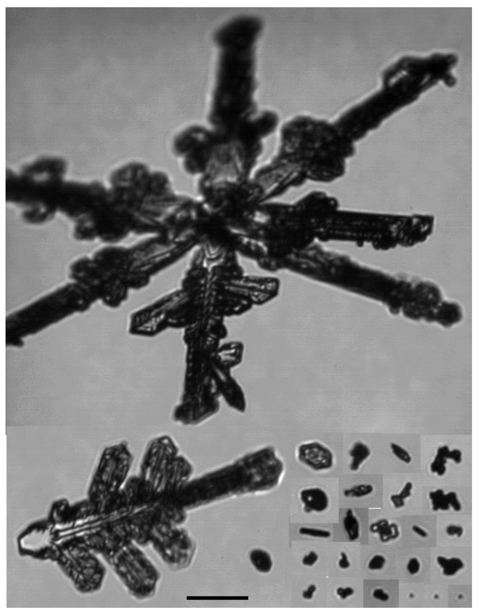
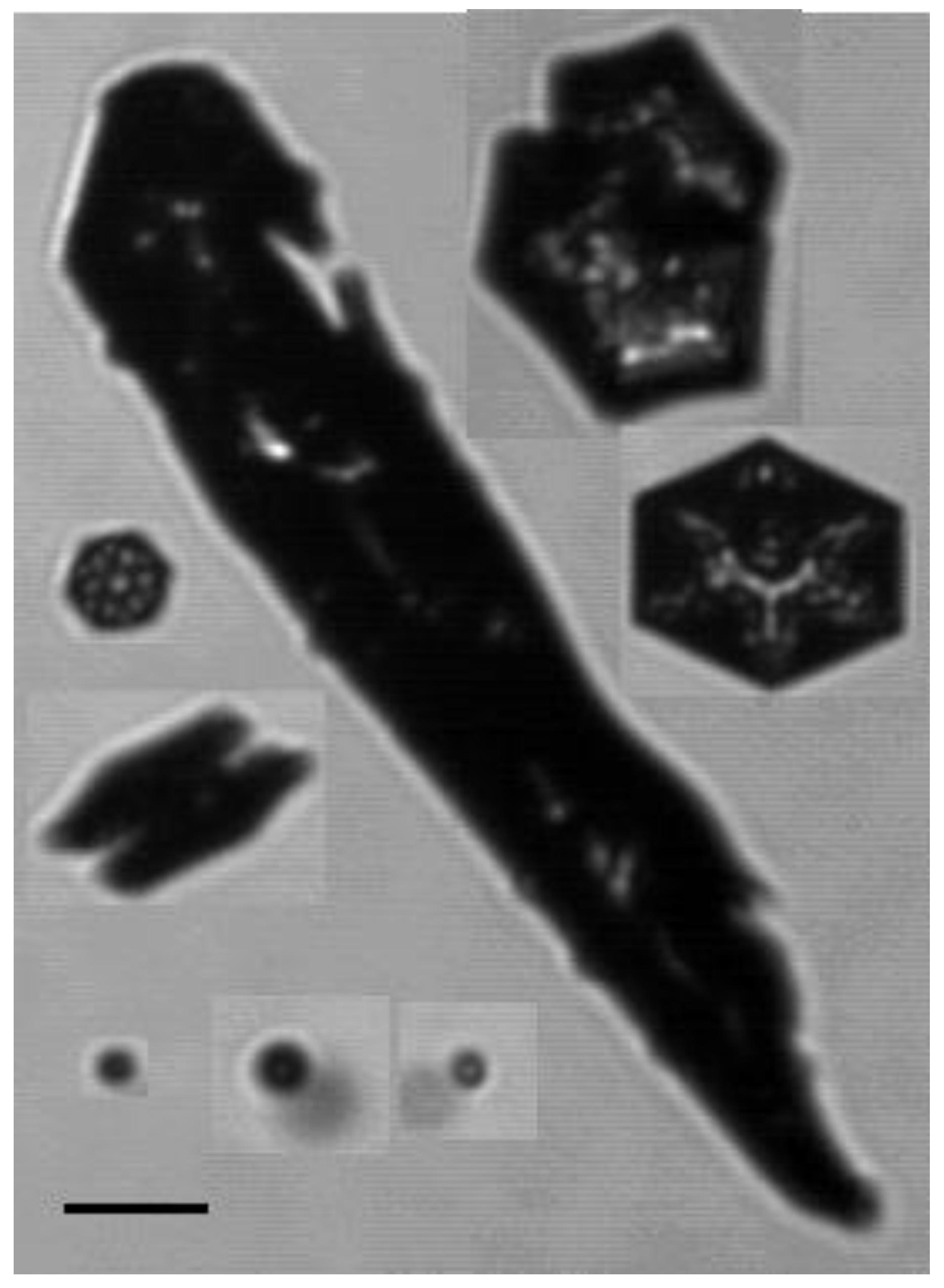
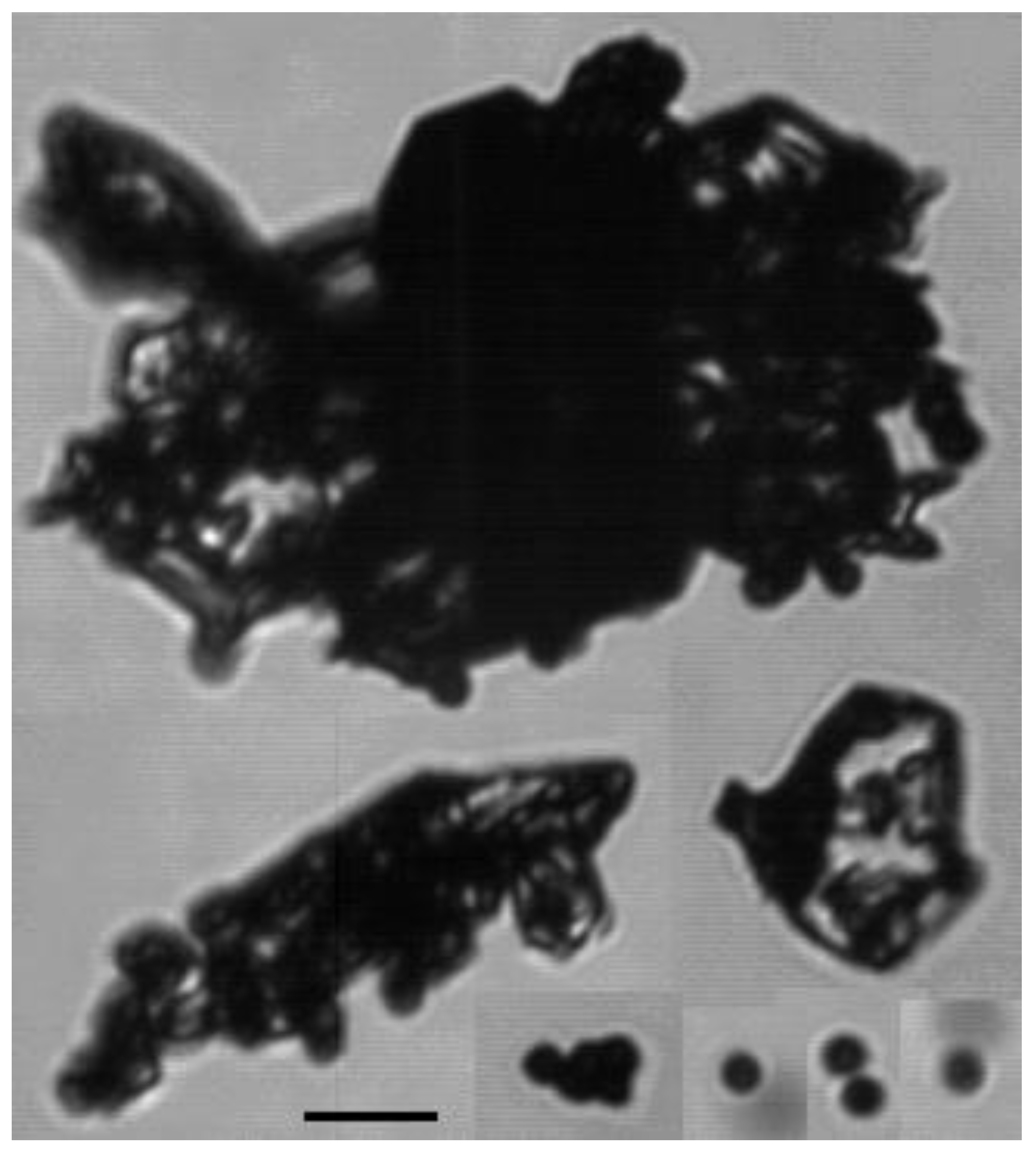
• Fluxes can be obtained from measured ice particle number concentrations. In cloud free cases, the most reasonable source is ice particles grown on the surface particularly when the wind speed threshold does not reach values necessary for initiation of blowing snow. CPI images recorded during suspected blowing snow events confirm that the particles are similar to those observed previously during blowing snow events, namely aged particles with rounded edges due to the transport through unsaturated air with respect to ice. Still, the low wind speeds as well as a missing correlation between wind speed and ice number concentration allow us to discard blowing snow as a mechanism for the measured high ice number concentrations. We therefore conclude that frost crystals growing on the snow surface are the likely source of the ice crystals, following Lloyd et al. [1].
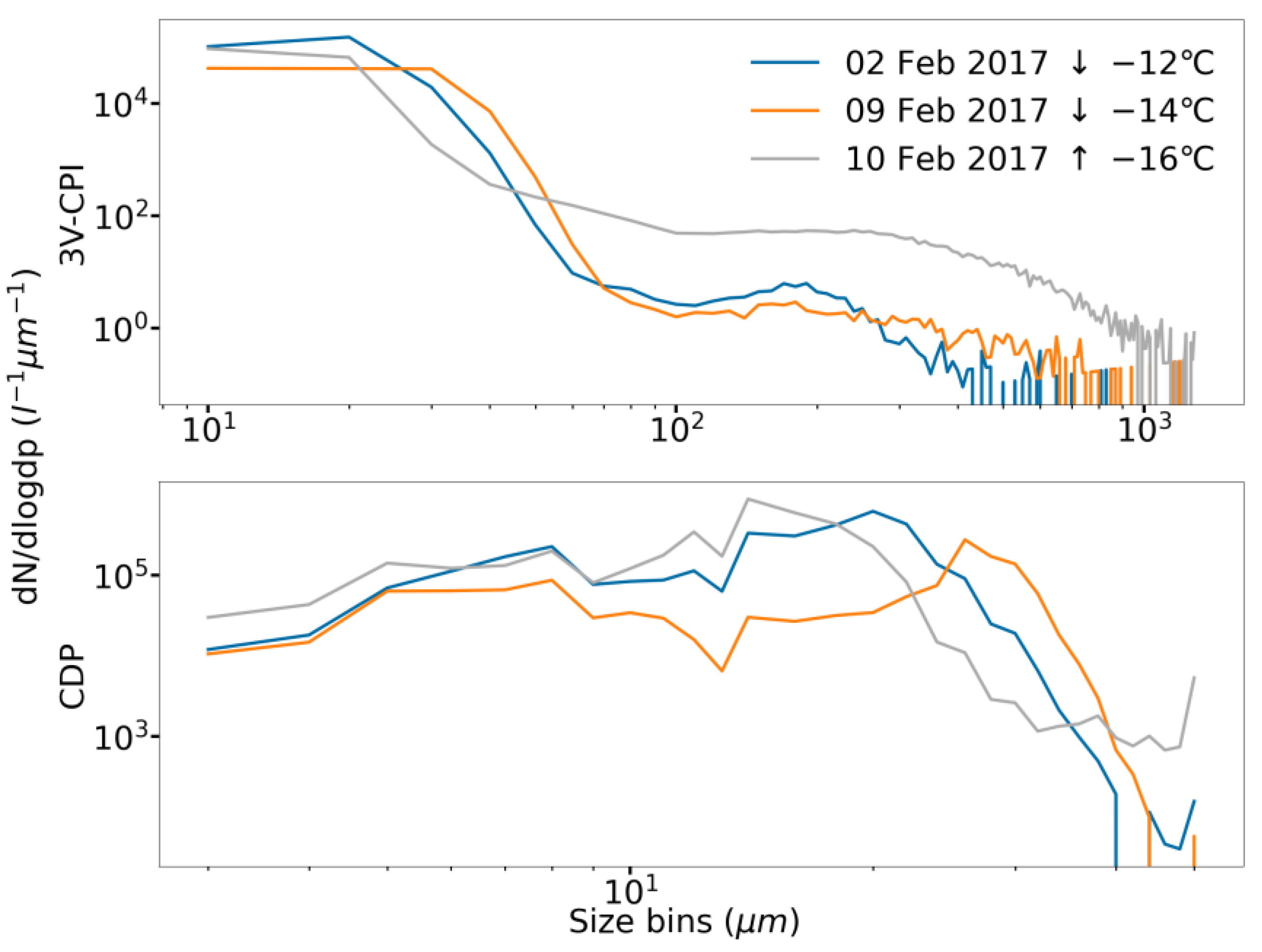
• A wide range of plate-like crystals is observed in the cloud, suggesting their origin is surface hoar frost rather than riming splintering on rocks and vegetation.
• Also, fluxes (with relevant values) do not always occur. It seems that it takes time for the surface source to form and reach a number density sufficient for the wind to begin generating a measurable upward flux. These upward fluxes also have to interact with an orographic cloud near enough to the surface to influence the ice number concentrations inside the cloud. The observed fluxes and conditions in which they occur are not generally consistent with blowing snow.
• In-cloud cases indicate strong positive and negative fluxes during an event are present most of the time. CPI images show similar ice particle habits present during each event. This leads to the conclusion that the Jungfraujoch research station resides too remote from the source of the ice particle fluxes so that the air mass sampled at the summit has become well-mixed.
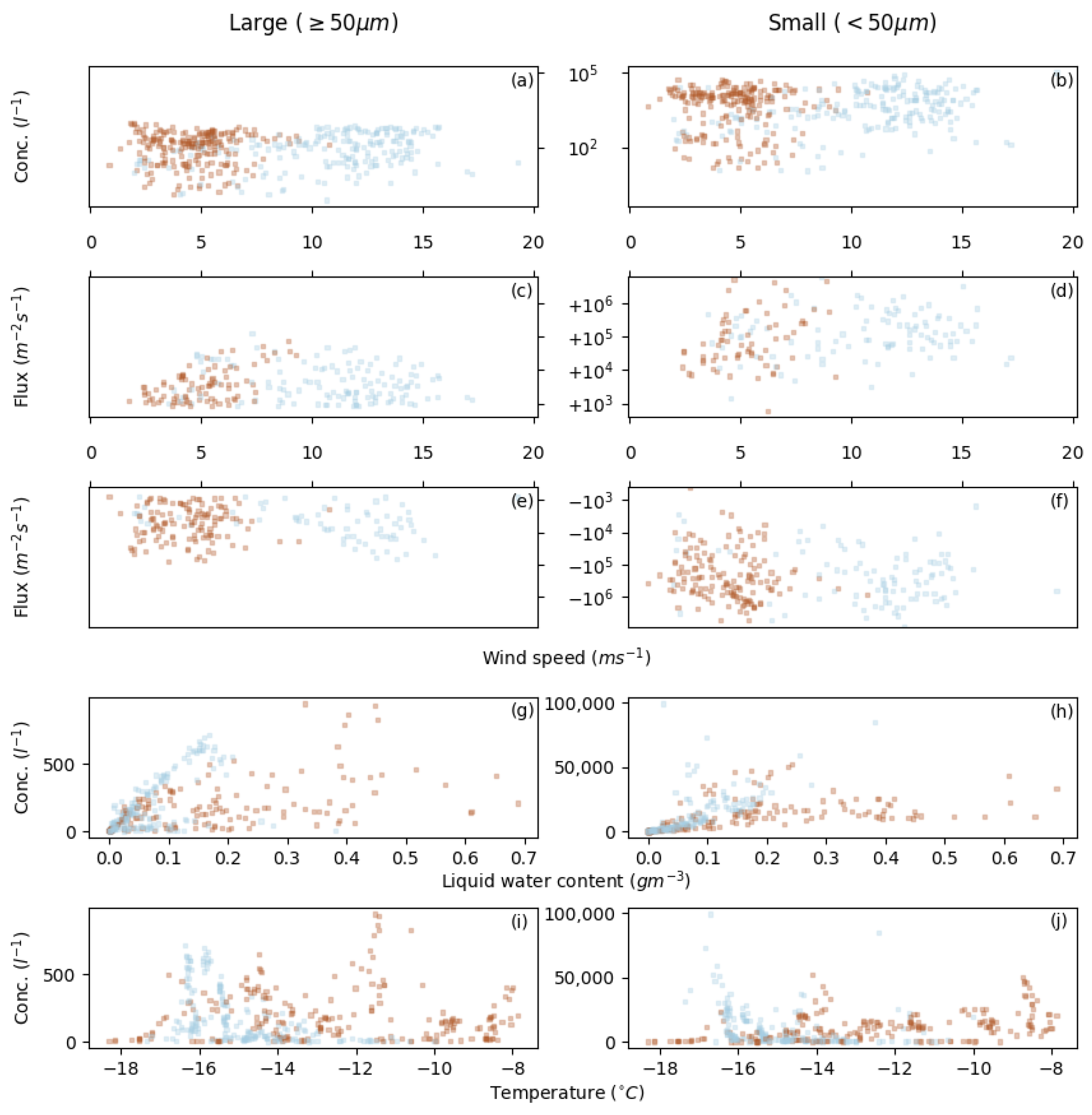
• Also, the high ice number concentration during cloud events masks the fluxes. On the one hand, downward fluxes of ice particles subdue local upward fluxes from the surface. On the other hand, events from the south produce high liquid water content with larger droplets that have downward motion. Because they are larger than 50 µm they are included into the calculation of the large particle fluxes. Hence, they influence the upward fluxes.
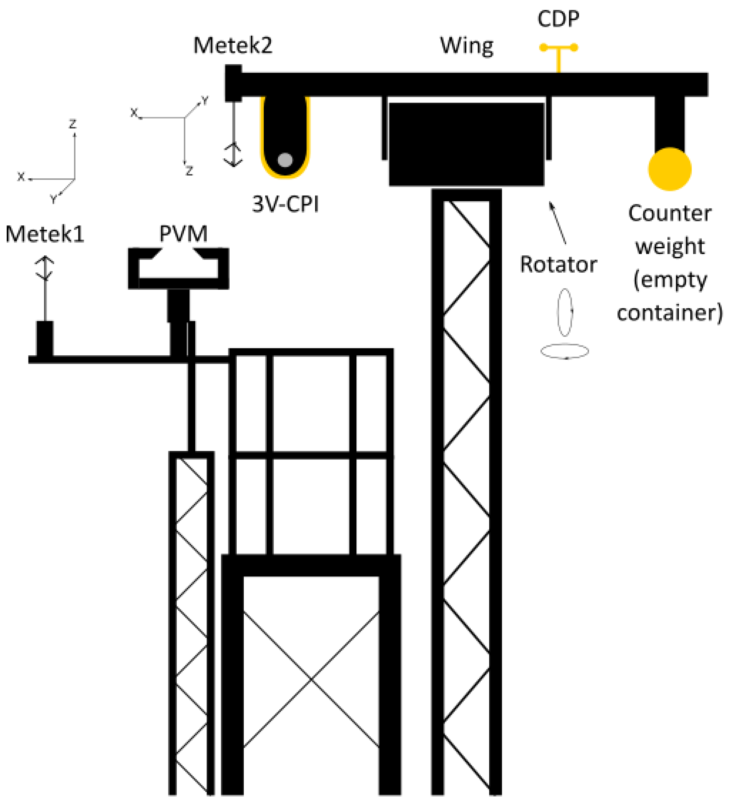
• The use of a 3D rotating wing is suited for the measurement of ice particles using a closed path shadow imager that is normally located underneath a wing of an airplane that has to be faced parallel to the mean wind field. For future work, we suggest improvements to such setups can include use of open-path cloud instruments, as closed-path instruments are more prone to shattering, although such artefacts can be removed using inter-particle arrival time analyses. Other potential particle sources, e.g., from above the Jungfraujoch, could be examined using contemporaneous ceilometer measurements along with local cloud base location. Particle concentrations upwind of the station would also confirm the results presented here.
• Calculating the fluxes for particles larger 50 μm with reasonably high values similar to the values that Farrington et al. [13] modelled (around 1 × 10³ m⁻²s⁻¹) strengthens and reaffirm the conclusion from previous publications for the existence of the surface fluxes mechanism. In particular, a surface flux of ice particles could explain the exceptionally high ice number concentration that is measured in orographic clouds.
• Hereby, it is still dubious if the origin of the upward flux is the growth of surface hoar and sublimation crystals. The riming effect might be an additional possible mechanism as the correlation between LWC and the concentration of large and also small particles suggests, as it also happens in the close proximity of the surface. More experiments closer to the origin or in the lab are therefore necessary to reveal more of the mechanism in detail.

References

1. Lloyd, G.; Choularton, T.W.; Bower, K.N.; Gallagher, M.W.; Connolly, P.J.; Flynn, M.; Farrington, R.; Crosier, J.; Schlenczek, O.; Fugal, J.; et al. The Origins of Ice Crystals Measured in Mixed-Phase Clouds at the High-Alpine Site Jungfraujoch. Atmos. Meas. Tech. 2015, 15, 12953–12969. [Google Scholar] [CrossRef] [Green Version]
2. Beck, A.; Henneberger, J.; Fugal, J.; David, R.O.; Lacher, L.; Lohmann, U. Impact of Surface and Near-Surface Processes on Ice Crystal Concentrations Measured at Mountain-Top Research Stations. Atmos. Meas. Tech. 2018, 18, 8909–8927. [Google Scholar] [CrossRef] [Green Version]
3. Conen, F.; Rodríguez, S.; Hüglin, C.; Henne, S.; Herrmann, E.; Bukowiecki, N.; Alewell, C. Atmospheric Ice Nuclei at the High-Altitude Observatory Jungfraujoch, Switzerland. Tellus B Chem. Phys. Meteorol. 2015, 67, 25014. [Google Scholar] [CrossRef]
4. Hallett, J.; Mossop, S.C. Production of Secondary Ice Particles during the Riming Process. Nature 1974, 249, 26–28. [Google Scholar] [CrossRef]
5. Vionnet, V.; Guyomarc’h, G.; Naaim Bouvet, F.; Martin, E.; Durand, Y.; Bellot, H.; Bel, C.; Puglièse, P. Occurrence of Blowing Snow Events at an Alpine Site over a 10-Year Period: Observations and Modelling. Adv. Water Resour. 2013, 55, 53–63. [Google Scholar] [CrossRef]
6. Geerts, B.; Pokharel, B.; Kristovich, D.A.R. Blowing Snow as a Natural Glaciogenic Cloud Seeding Mechanism. Mon. Weather. Rev. 2015, 143, 5017–5033. [Google Scholar] [CrossRef]
7. Lee, X.; Finnigan, J.; Paw, U.K.T. Handbook of Micrometeorology: A Guide for Surface Flux Measurement and Analysis; Springer Science + Business Media, Inc.: Berlin/Heidelberg, Germany, 2005; Volume 29, ISBN 978-1-4020-2264-7. [Google Scholar]
8. Baltensperger, U.; Schwikowski, M.; Jost, D.T.; Nyeki, S.; Gäggeler, H.W.; Poulida, O. Scavenging of Atmospheric Constituents in Mixed Phase Clouds at the High-Alpine Site Jungfraujoch Part I. Atmos. Environ 1998, 32, 3975–3983. [Google Scholar] [CrossRef]
9. Hinz, K.P.; Trimborn, A.; Weingartner, E.; Henning, S.; Baltensperger, U.; Spengler, B. Aerosol Single Particle Composition at the Jungfraujoch. J. Aerosol Sci. 2005, 36, 123–145. [Google Scholar] [CrossRef]
10. Hoyle, C.R.; Webster, C.S.; Rieder, H.E.; Nenes, A.; Hammer, E.; Herrmann, E.; Gysel, M.; Bukowiecki, N.; Weingartner, E.; Steinbacher, M.; et al. Chemical and Physical Influences on Aerosol Activation in Liquid Clouds: A Study Based on Observations from the Jungfraujoch, Switzerland. Atmos. Chem. Phys. 2016, 16, 4043–4061. [Google Scholar] [CrossRef] [Green Version]
11. Kupiszewski, P.; Zanatta, M.; Mertes, S.; Vochezer, P.; Lloyd, G.; Schneider, J.; Schenk, L.; Schnaiter, M.; Baltensperger, U.; Weingartner, E.; et al. Ice Residual Properties in Mixed-Phase Clouds at the High-Alpine Jungfraujoch Site. J. Geophys. Res. 2016, 121, 12,343–12,362. [Google Scholar] [CrossRef] [Green Version]
12. Choularton, T.W.; Bower, K.N.; Weingartner, E.; Crawford, I.; Coe, H.; Gallagher, M.W.; Flynn, M.; Crosier, J.; Connolly, P.; Targino, A.; et al. The Influence of Small Aerosol Particles on the Properties of Water and Ice Clouds. Faraday Discuss 2007, 137, 205–222. [Google Scholar] [CrossRef] [PubMed]
13. Farrington, R.J.; Connolly, P.J.; Lloyd, G.; Bower, K.N.; Flynn, M.J.; Gallagher, M.W.; Field, P.R.; Dearden, C.; Choularton, T.W. Comparing Model and Measured Ice Crystal Concentrations in Orographic Clouds during the INUPIAQ Campaign. Atmos. Chem. Phys. 2016, 16, 4945–4966. [Google Scholar] [CrossRef] [Green Version]
14. Lawson, R.P.; O’Connor, D.; Zmarzly, P.; Weaver, K.; Baker, B.; Mo, Q.; Jonsson, H. The 2D-S (Stereo) Probe: Design and Preliminary Tests of a New Airborne, High-Speed, High-Resolution Particle Imaging Probe. J. Atmos. Ocean. Technol. 2006, 23, 1462–1477. [Google Scholar] [CrossRef] [Green Version]
15. Lance, S.; Brock, C.A.; Rogers, D.; Gordon, J.A. Water Droplet Calibration of the Cloud Droplet Probe (CDP) and in-Flight Performance in Liquid, Ice and Mixed-Phase Clouds during ARCPAC. Atmos. Meas. Tech. 2010, 3, 1683–1706. [Google Scholar] [CrossRef] [Green Version]
16. Gerber, H. Direct Measurement of Suspended Particulate Volume Concentration and Far-Infrared Extinction Coefficient with a Laser-Diffraction Instrument. Appl. Opt. 1991, 30, 4824–4831. [Google Scholar] [CrossRef]
17. Beswick, K.M.; Hargreaves, K.J.; Gallagher, M.W.; Choularton, T.W.; Fowler, D. Size-Resolved Measurements of Cloud Droplet Deposition Velocity to a Forest Canopy Using an Eddy Correlation Technique. Q. J. R. Meteorol. Soc. 1991, 117, 623–645. [Google Scholar] [CrossRef]
18. Vong, R.; Kowalski, A.S. Eddy Correlation Measurements of Size-Dependent Cloud Droplet Turbulent Fluxes to Complex Terrain. Tellus B 1995, 47, 331–352. [Google Scholar] [CrossRef] [Green Version]
19. Kowalski, A.S.; Anthoni, P.M.; Vong, R.J.; Delany, A.C.; Maclean, G.D. Deployment and Evaluation of a System for Ground-Based Measurement of Cloud Liquid Water Turbulent Fluxes. J. Atmos. Ocean. Technol. 1997, 14, 468–479. [Google Scholar] [CrossRef]
20. Klemm, O.; Wrzesinsky, T.; Scheer, C. Fog Water Flux at a Canopy Top: Direct Measurement versus One-Dimensional Model. Atmos. Environ. 2005, 39, 5375–5386. [Google Scholar] [CrossRef]
21. Pryor, S.C.; Gallagher, M.; Sievering, H.; Larsen, S.E.; Barthelmie, R.J.; Birsan, F.; Nemitz, E.; Rinne, J.; Kulmala, M.; Grönholm, T.; et al. A Review of Measurement and Modelling Results of Particle Atmosphere-Surface Exchange. Tellus B Chem. Phys. Meteorol. 2008, 60B, 42–75. [Google Scholar] [CrossRef]
22. Gerber, H.; DeMott, P.J. Response of FSSP-100 and PVM-100A to Small Ice Crystals. J. Atmos. Ocean. Technol. 2014, 31, 2145–2155. [Google Scholar] [CrossRef]
23. Gallet, J.C.; Domine, F.; Savarino, J.; Dumont, M.; Brun, E. The Growth of Sublimation Crystals and Surface Hoar on the Antarctic Plateau. Cryosphere 2014, 8, 1205–1215. [Google Scholar] [CrossRef] [Green Version]
24. Style, R.W.; Worster, M.G. Frost Flower Formation on Sea Ice and Lake Ice. Geophys. Res. Lett. 2009, 36, 20–23. [Google Scholar] [CrossRef] [Green Version]
25. Gallagher, M.W.; Choularton, T.W.; Morse, A.P.; Fowler, D. Measurements of the Size Dependence of Cloud Droplet Deposition at a Hill Site. Q. J. R. Meteorol. Soc. 1988, 114, 1291–1303. [Google Scholar] [CrossRef]
26. Gallagher, M.W.; Beswick, K.M.; Choularton, T.W. Measurement and Modelling of Cloudwater Deposition to a Snow-Covered Forest Canopy. Atmos. Environ. Part A Gen. Top. 1992, 26, 2893–2903. [Google Scholar] [CrossRef]
27. Gallagher, M.W.; Beswick, K.; Choularton, T.W.; Coe, H.; Fowler, D.; Hargreaves, K. Measurements and Modelling of Cloudwater Deposition to Moorland and Forests. Environ. Pollut. 1992, 75, 97–107. [Google Scholar] [CrossRef]
28. Holwerda, F.; Burkard, R.; Eugster, W.; Scatena, F.N.; Meesters, A.G.C.A.; Bruijnzeel, L.A. Estimating Fog Deposition at a Puerto Rican Elfin Cloud Forest Site: Comparison of the Water Budget and Eddy Covariance Methods. Hydrol. Process. 2006, 20, 2669–2692. [Google Scholar] [CrossRef]
29. Schmidt, A.; Klemm, O. Direct Determination of Highly Size-Resolved Turbulent Particle Fluxes with the Disjunct Eddy Covariance Method and a 12—Stage Electrical Low Pressure Impactor. Atmos. Chem. Phys. Discuss. 2008, 8, 8997–9034. [Google Scholar] [CrossRef] [Green Version]
30. Wilczak, J.M.; Oncley, S.P.; Stage, S.A. Sonic Anemometer Tilt Correction Algorithms. Bound. Layer Meteorol 2001, 99, 127–150. [Google Scholar] [CrossRef]
31. Finnigan, J.J. A Re-Evaluation of Long-Term Flux Measurement Techniques Part II: Coordinate Systems. Bound. Layer Meteorol 2004, 113, 1–41. [Google Scholar] [CrossRef]
32. Crosier, J.; Bower, K.N.; Choularton, T.W.; Westbrook, C.D.; Connolly, P.J.; Cui, Z.Q.; Crawford, I.P.; Capes, G.L.; Coe, H.; Dorsey, J.R.; et al. Observations of Ice Multiplication in a Weakly Convective Cell Embedded in Supercooled Mid-Level Stratus. Atmos. Chem. Phys. 2011, 11, 257–273. [Google Scholar] [CrossRef] [Green Version]
33. Korolev, A. Reconstruction of the Sizes of Spherical Particles from Their Shadow Images. Part I: Theoretical Considerations. J. Atmos. Ocean. Technol. 2007, 24, 376–389. [Google Scholar] [CrossRef]
34. Connolly, P.J.; Flynn, M.J.; Ulanowski, Z.; Choularton, T.W.; Gallagher, M.W.; Bower, K.N. Calibration of the Cloud Particle Imager Probes Using Calibration Beads and Ice Crystal Analogs: The Depth of Field. J. Atmos. Ocean. Technol. 2007, 24, 1860–1879. [Google Scholar] [CrossRef]
35. O’Shea, S.J.; Crosier, J.; Dorsey, J.; Schledewitz, W.; Crawford, I.; Borrmann, S.; Cotton, R.; Bansemer, A. Revisiting Particle Sizing Using Greyscale Optical Array Probes: Evaluation Using Laboratory Experiments and Synthetic Data. Atmos. Meas. Tech. 2019, 12, 3067–3079. [Google Scholar] [CrossRef] [Green Version]
36. Korolev, A.V.; Emery, E.F.; Strapp, J.W.; Cober, S.G.; Isaac, G.A. Quantification of the Effects of Shattering on Airborne Ice Particle Measurements. J. Atmos. Ocean. Technol. 2013, 30, 2527–2553. [Google Scholar] [CrossRef]
37. Lawson, R.P. Effects of Ice Particles Shattering on the 2D-S Probe. Atmos. Meas. Tech. 2011, 4, 1361–1381. [Google Scholar] [CrossRef] [Green Version]
38. Rogers, D.C.; Vali, G. Ice Crystal Production by Mountain Surfaces. J. Clim. Appl. Meteorol. 1987, 26, 1152–1168. [Google Scholar] [CrossRef]
Figure 1. High altitude research station Jungfraujoch (46°32′51.0″N 7°59′06.2″E) seen from above with the Aletschgletscher (Aletsch Glacier) to the south. The black circle with a 25 m radius marks the location of the station on top of the ridge and its periphery.
Atmosphere 14 00474 g001
Figure 2. Overview of the instruments (see Table 1) and their position within the experimental setup. The wing is located at a height of 3 m.
Atmosphere 14 00474 g002
Figure 3. Example ogive plot from the 30 January 2017. It shows the normalized frequency f times the co-spectra co (solid line) and corresponding normalized ogive og (dashed line) versus the frequency on the bottom and corresponding period on the top axes. After eight minutes, the ogive approaches one and does not increase significantly.
Atmosphere 14 00474 g003
Figure 4. Box plots of the eight-minute flux periods for the whole campaign, divided into positive (↑) and negative (↓) fluxes. Horizontal lines mark the median; points represent the mean; whiskers mark the most extreme, non-outlier data points; fliers (circles) represent data that extend beyond the whiskers.
Atmosphere 14 00474 g004
Figure 5. Scatter plot between concentration and flux vs. wind speed (af), concentration vs. LWC (g,h), and concentration vs. temperature (i,j) for particles larger 50 μm (left panels) and smaller 50 μm (right panels). Each point represents an 8 min mean (blue: from the south, red: from the north).
Atmosphere 14 00474 g005
Figure 6. Normalized size distribution of the 3V-CPI and the CDP for all sizes from 2.3 up to 1280 μm for three days with positive (↑) and negative (↓) flux directions.
Atmosphere 14 00474 g006
Figure 7. CPI images of typical ice particles and water droplets for LWC > 0.21 gm−3 for positive flux on the 10 February. The horizontal scale (bottom of figure) indicates 100 μm.
Atmosphere 14 00474 g007
Figure 8. Same as Figure 6 but for the 2 February and negative flux.
Atmosphere 14 00474 g008
Figure 9. Same as Figure 6 but for the 9 February and negative flux.
Atmosphere 14 00474 g009