
Turbulent Inflow Generation for Large-Eddy Simulation of Winds around Complex Terrain

Abstract
:1. Introduction
2. Numerical Formulation
3. Computational Setup
4. Results
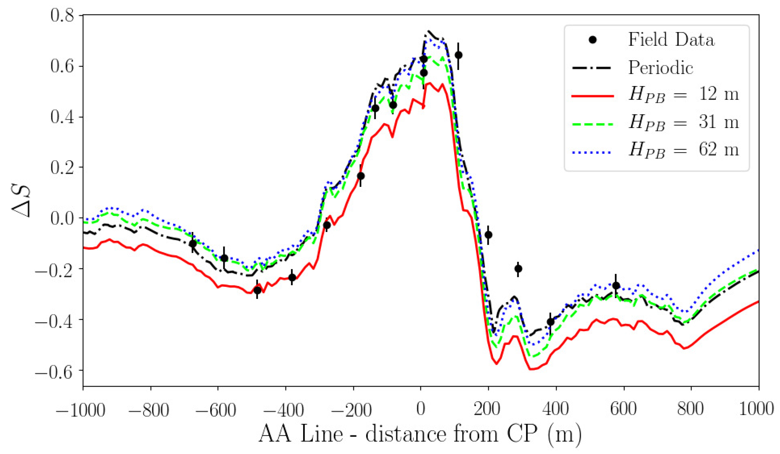
4.1. Askervein Hill
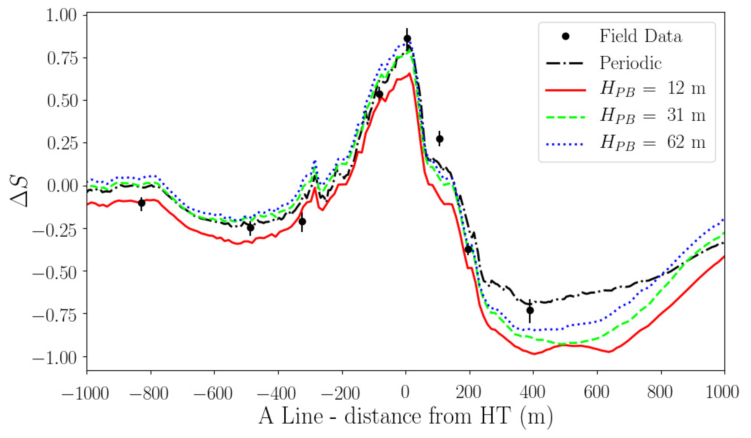
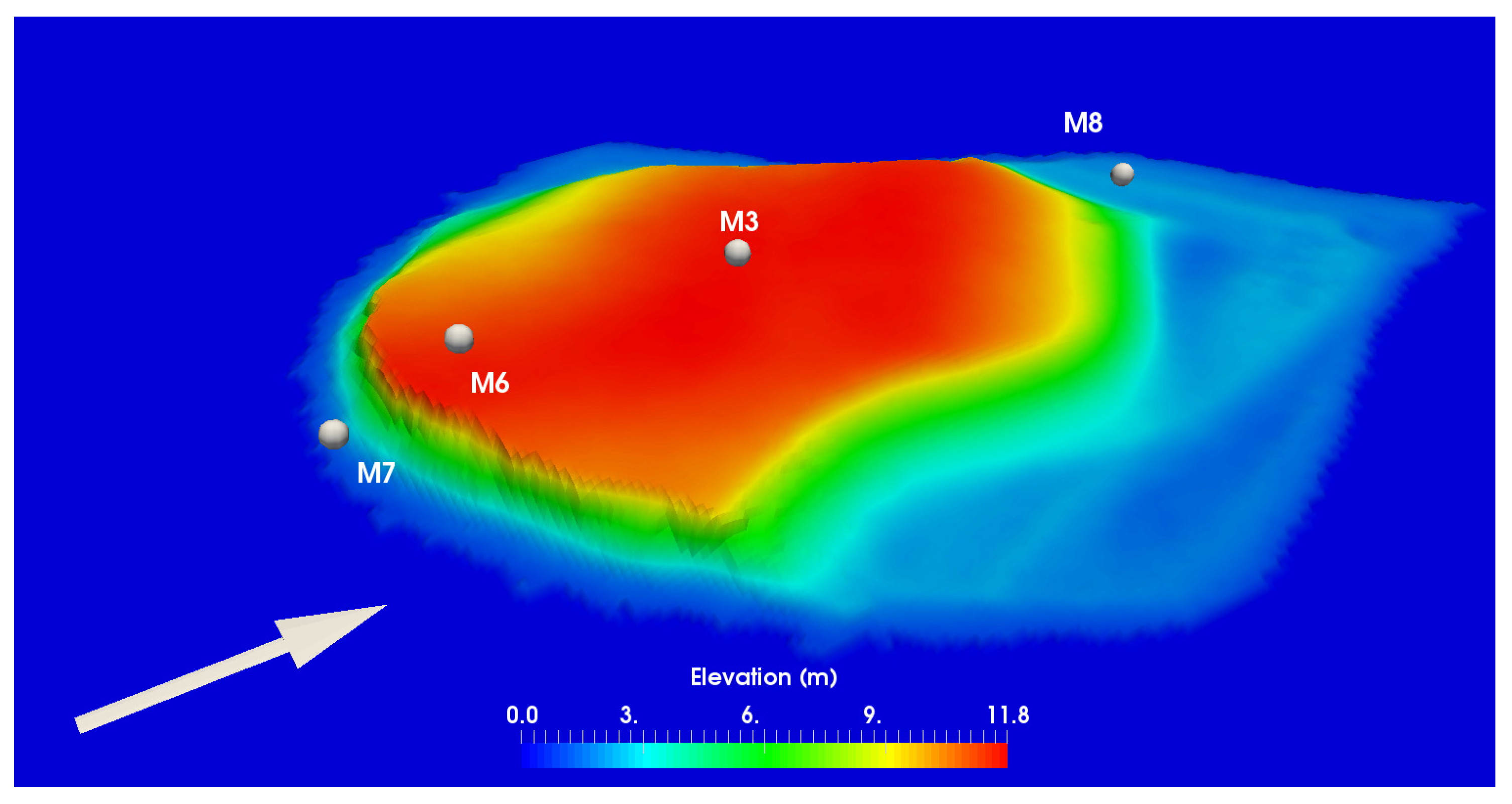
4.2. Bolund Hill
5. Discussion
6. Conclusions
Author Contributions
Funding
Institutional Review Board Statement
Informed Consent Statement
Data Availability Statement
Conflicts of Interest
References
- Mehta, D.; Van Zuijlen, A.; Koren, B.; Holierhoek, J.; Bijl, H. Large eddy simulation of wind farm aerodynamics: A review. J. Wind Eng. Ind. Aerod. 2014, 133, 1–17. [Google Scholar] [CrossRef]
- Shikhovtsev, A.Y.; Kovadlo, P.G.; Lezhenin, A.A.; Korobov, O.A.; Kiselev, A.V.; Russkikh, I.V.; Kolobov, D.Y.; Shikhovtsev, M.Y. Influence of Atmospheric Flow Structure on Optical Turbulence Characteristics. Appl. Sci. 2023, 13, 1282. [Google Scholar] [CrossRef]
- Keating, A.; Piomelli, U.; Balaras, E.; Kaltenbach, H.J. A priori and a posteriori tests of inflow conditions for large-eddy simulation. Phys. Fluids 2004, 16, 4696–4712. [Google Scholar] [CrossRef]
- Tabor, G.; Baba-Ahmadi, M. Inlet conditions for large eddy simulation: A review. Comput. Fluids 2010, 39, 553–567. [Google Scholar] [CrossRef]
- Wu, X. Inflow turbulence generation methods. Annu. Rev. Fluid Mech. 2017, 49, 23–49. [Google Scholar] [CrossRef]
- Lopes, A.S.; Palma, J.; Castro, F. Simulation of the Askervein flow. Part 2: Large-eddy simulations. Bound.-Layer Meteorol. 2007, 125, 85–108. [Google Scholar] [CrossRef]
- Diebold, M.; Higgins, C.; Fang, J.; Bechmann, A.; Parlange, M.B. Flow over hills: A large-eddy simulation of the Bolund case. Bound.-Layer Meteorol. 2013, 148, 177–194. [Google Scholar] [CrossRef] [Green Version]
- Porté-Agel, F.; Wu, Y.T.; Chen, C.H. A numerical study of the effects of wind direction on turbine wakes and power losses in a large wind farm. Energies 2013, 6, 5297–5313. [Google Scholar] [CrossRef] [Green Version]
- Munters, W.; Meneveau, C.; Meyers, J. Turbulent inflow precursor method with time-varying direction for large-eddy simulations and applications to wind farms. Bound.-Layer Meteorol. 2016, 159, 305–328. [Google Scholar] [CrossRef] [Green Version]
- Lund, T.S.; Wu, X.; Squires, K.D. Generation of inflow data for spatially-developing boundary layer simulations. J. Comput. Phys. 1998, 140, 233–258. [Google Scholar] [CrossRef] [Green Version]
- Mayor, S.; Spalart, P.; Tripoli, G. Application of a perturbation recycling method in the large-eddy simulation of a mesoscale convective internal boundary layer. J. Atmos. Sci. 2002, 59, 2385–2395. [Google Scholar] [CrossRef]
- Araya, G.; Castillo, L.; Meneveau, C.; Jansen, K. A dynamic multi-scale approach for turbulent inflow boundary conditions in spatially developing flows. J. Fluid Mech. 2011, 670, 581–605. [Google Scholar] [CrossRef]
- Park, J.; Basu, S.; Manuel, L. Large-eddy simulation of stable boundary layer turbulence and estimation of associated wind turbine loads. Wind Energy 2014, 17, 359–384. [Google Scholar] [CrossRef]
- Mann, J. Wind field simulation. Probabilist. Eng. Mech. 1998, 13, 269–282. [Google Scholar] [CrossRef]
- Xie, Z.T.; Castro, I.P. Large-eddy simulation for flow and dispersion in urban streets. Atmos. Environ. 2009, 43, 2174–2185. [Google Scholar] [CrossRef] [Green Version]
- Jarrin, N.; Prosser, R.; Uribe, J.C.; Benhamadouche, S.; Laurence, D. Reconstruction of turbulent fluctuations for hybrid RANS/LES simulations using a synthetic-eddy method. Int. J. Heat Fluid Fl. 2009, 30, 435–442. [Google Scholar] [CrossRef] [Green Version]
- Poletto, R.; Craft, T.; Revell, A. A new divergence free synthetic eddy method for the reproduction of inlet flow conditions for LES. Flow Turbul. Combust. 2013, 91, 519–539. [Google Scholar] [CrossRef]
- Muñoz-Esparza, D.; Kosović, B.; Mirocha, J.; van Beeck, J. Bridging the Transition from Mesoscale to Microscale Turbulence in Numerical Weather Prediction Models. Bound.-Layer Meteorol. 2014, 153, 409–440. [Google Scholar] [CrossRef]
- Muñoz-Esparza, D.; Kosović, B.; van Beeck, J.; Mirocha, J. A stochastic perturbation method to generate inflow turbulence in large-eddy simulation models: Application to neutrally stratified atmospheric boundary layers. Phys. Fluids 2015, 27, 035102. [Google Scholar] [CrossRef]
- Umphrey, C.; Senocak, I. Turbulent Inflow Generation for the Large-eddy Simulation Technique Through Globally Neutral Buoyancy Perturbations. In Proceedings of the 54th AIAA SciTech Forum, American Institute of Aeronautics and Astronautics, San Diego, CA, USA, 4–8 January 2016. [Google Scholar] [CrossRef]
- Deleon, R.; Umphrey, C.; Senocak, I. Turbulent inflow generation through buoyancy perturbations with colored noise. AIAA J. 2019, 57, 532–542. [Google Scholar] [CrossRef]
- Senocak, I.; Ackerman, A.; Kirkpatrick, M.; Stevens, D.; Mansour, N. Study of near-surface models for large-eddy simulations of a neutrally stratified atmospheric boundary layer. Bound.-Layer Meteorol. 2007, 124, 405–424. [Google Scholar] [CrossRef]
- Umphrey, C.; DeLeon, R.; Senocak, I. Direct Numerical Simulation of Turbulent Katabatic Slope Flows with an Immersed-Boundary Method. Bound.-Layer Meteorol. 2017, 164, 367–382. [Google Scholar] [CrossRef] [Green Version]
- DeLeon, R.; Sandusky, M.; Senocak, I. Simulations of Turbulent Flow Over Complex Terrain Using an Immersed-Boundary Method. Bound.-Layer Meteorol. 2018, 167, 399–420. [Google Scholar] [CrossRef]
- Thibault, J.C.; Senocak, I. Accelerating incompressible flow computations with a Pthreads-CUDA implementation on small-footprint multi-GPU platforms. J. Supercomput. 2012, 59, 693–719. [Google Scholar] [CrossRef]
- Jacobsen, D.; Senocak, I. Multi-level parallelism for incompressible flow computations on GPU clusters. Parallel Comput. 2013, 39, 1–20. [Google Scholar] [CrossRef] [Green Version]
- DeLeon, R.; Jacobsen, D.; Senocak, I. Large-eddy simulations of turbulent incompressible flows on GPU clusters. Comput. Sci. Eng. 2013, 15, 26–33. [Google Scholar] [CrossRef]
- Jacobsen, D.A.; Senocak, I. A full-depth amalgamated parallel 3D geometric multigrid solver for GPU clusters. In Proceedings of the 49th AIAA Aerospace Science Meeting, Orlando, FL, USA, 4–7 January 2011. [Google Scholar]
- Munters, W.; Meneveau, C.; Meyers, J. Shifted periodic boundary conditions for simulations of wall-bounded turbulent flows. Phys. Fluids 2016, 28, 025112. [Google Scholar] [CrossRef] [Green Version]
- Taylor, P.; Teunissen, H. The Askervein Hill project: Overview and background data. Bound.-Layer Meteorol. 1987, 39, 15–39. [Google Scholar] [CrossRef]
- Mickle, R.; Cook, N.; Hoff, A.; Jensen, N.; Salmon, J.; Taylor, P.; Tetzlaff, G.; Teunissen, H. The Askervein Hill Project: Vertical profiles of wind and turbulence. Bound.-Layer Meteorol. 1988, 43, 143–169. [Google Scholar] [CrossRef]
- Salmon, J.; Bowen, A.; Hoff, A.; Johnson, R.; Mickle, R.; Taylor, P.; Tetzlaff, G.; Walmsley, J. The Askervein Hill project: Mean wind variations at fixed heights above ground. Bound.-Layer Meteorol. 1988, 43, 247–271. [Google Scholar] [CrossRef]
- Walmsley, J.; Taylor, P. Boundary-layer flow over topography: Impacts of the Askervein study. In Boundary-Layer Meteorology 25th Anniversary Volume, 1970–1995; Springer: Berlin/Heidelberg, Germany, 1996; pp. 291–320. [Google Scholar]
- Berg, J.; Mann, J.; Bechmann, A.; Courtney, M.; Jørgensen, H. The Bolund Experiment, Part I: Flow Over a Steep, Three-Dimensional Hill. Bound.-Layer Meteorol. 2011, 141, 219–243. [Google Scholar] [CrossRef] [Green Version]
- Bechmann, A.; Sørensen, N.; Berg, J.; Mann, J.; Réhoré, P.E. The Bolund Experiment, Part II: Blind Comparison of Microscale Flow Models. Bound.-Layer Meteorol. 2011, 141, 245–271. [Google Scholar] [CrossRef] [Green Version]
- Benocci, C.; Pinelli, A. The role of the forcing term in the large eddy simulation of equilibrium channel flow. In Engineering Turbulence Modeling and Experiments; Rodi, W., Ganic, E., Eds.; Elsevier: New York, NY, USA, 1990; pp. 287–296. [Google Scholar]
- Taylor, P.; Teunissen, H. The Askervein Hill Project: Report on the September/October 1983, Main Field Experiment; Atmospheric Environment Service: Downsview, ON, Canada, 1985. [Google Scholar]


| Case | (m) | (m) | (m) | PB Depth |
|---|---|---|---|---|
| Ask1 | 12 | 23 | 23 | 3 |
| Ask2 | 38 | 76 | 76 | 3 |
| Ask3 | 62 | 123 | 123 | 3 |
| Case | (m) | (m) | (m) | PB Depth |
|---|---|---|---|---|
| Bol1 | 2 | 4 | 4 | 3 |
| Bol2 | 17 | 35 | 35 | 3 |
Disclaimer/Publisher’s Note: The statements, opinions and data contained in all publications are solely those of the individual author(s) and contributor(s) and not of MDPI and/or the editor(s). MDPI and/or the editor(s) disclaim responsibility for any injury to people or property resulting from any ideas, methods, instructions or products referred to in the content. |
© 2023 by the authors. Licensee MDPI, Basel, Switzerland. This article is an open access article distributed under the terms and conditions of the Creative Commons Attribution (CC BY) license (https://creativecommons.org/licenses/by/4.0/).
Share and Cite
Senocak, I.; DeLeon, R. Turbulent Inflow Generation for Large-Eddy Simulation of Winds around Complex Terrain. Atmosphere 2023, 14, 447. https://doi.org/10.3390/atmos14030447
Senocak I, DeLeon R. Turbulent Inflow Generation for Large-Eddy Simulation of Winds around Complex Terrain. Atmosphere. 2023; 14(3):447. https://doi.org/10.3390/atmos14030447
Chicago/Turabian StyleSenocak, Inanc, and Rey DeLeon. 2023. "Turbulent Inflow Generation for Large-Eddy Simulation of Winds around Complex Terrain" Atmosphere 14, no. 3: 447. https://doi.org/10.3390/atmos14030447