Article

Ensemble of Below-Cloud Scavenging Models for Assessing the Uncertainty Characteristics in Wet Raindrop Deposition Modeling

Nuclear Safety Institute of the Russian Academy of Sciences (IBRAE RAN), 115191 Moscow, Russia
*
Author to whom correspondence should be addressed.
Atmosphere 2023, 14(2), 398; https://doi.org/10.3390/atmos14020398
Submission received: 27 January 2023 / Revised: 14 February 2023 / Accepted: 15 February 2023 / Published: 18 February 2023

Abstract

:
This work is devoted to the development of an ensemble of below-cloud scavenging models of pollutant aerosol transport into the atmosphere. Among other factors contributing to the uncertainty of the forecasts of the dispersion and deposition of technogenic gas-aerosol releases in the atmosphere, precipitation scavenging is one of the least studied and, in case of precipitation, can be the dominant mechanism for aerosol deposition. To form the ensemble of below-cloud scavenging models, appropriate experimental data, raindrop-aerosol capture models, raindrop terminal velocity parameterizations, and raindrop size distributions were chosen. The pool of models was prepared and then evaluated to adequately describe the experimental data using statistical analysis. Rank diagrams were used to analyze the adequacy of meteorological ensembles; together with the ensemble distribution construction, they allowed selecting the groups of models with such properties as to produce unbiased estimates and dispersion corresponding to the dispersion of the experimental data. The model calculations of the concentration fraction deposited due to below-cloud scavenging were performed using a log-normal distribution with characteristics corresponding to those observed during the accidents at the Chernobyl NPP and Fukushima-1 NPP. The results were compared with those obtained using the models of the NAME and FLEXPART codes. The results of this work can be used to improve the current approaches applied for modelling the distribution of pollutants in the atmosphere in the case of emergency, enhancing the reliability of forecasts by taking into account uncertainties in the results. The formed multi-model ensemble will be included in the decision support system used in responding to releases of radioactive substances into the atmosphere.

1. Introduction

Atmospheric transport modeling is one of the most important tasks of emergency preparedness and response [1,2] because atmospheric transport is the fastest way to deliver pollutants from the source to humans. Atmospheric transport modeling is performed using diagnostic or predictive weather forecast models, which generally determine the quality of the modeling. Depending on the problem, the forecast can be considered on different time scales, from “nowcasting” [3,4] for early detection of warning situations, to medium-range forecasting [5,6], which can be used for assessments of possible hazards to human health due to pollutant emissions, and finally long-term forecasts [7,8] for long-term safety analysis issues. Using models of atmospheric transport, the parameters of pollution of environmental objects are modeled. Important parameters such as surface deposition density and time-integrated concentration are used for assessment of the population exposure and hence the population safety [9]. The accuracy (mean and dispersion) of such estimates is studied in terms of processes that affect the result: turbulent and advective transport [10,11], dry deposition [12,13,14], chemical transformations [15,16], and precipitation scavenging [17,18]. At present, we know the accuracy of the models describing the turbulent transport for the landscapes, where the Monin–Obukhov similarity theory [19] is valid; dry deposition for areas with typified landscape conditions [20]; and wet deposition for precipitations that are relatively homogeneous over composition and territory [21]. In practice, when modeling the distribution of atmospheric releases during the accident at the Fukushima-1 NPP, the differences between the actual data and forecasts differed by orders of magnitude or more due to inaccuracy of knowledge about the source term [22] as well as to the inaccuracy of physical processes modeling [23]. An ensemble forecast [24] was developed to solve such problems, taking into account all uncertainties (inaccuracy of the initial data and inaccuracy of modeling processes). It was previously used for modeling weather conditions [25], to obtain the weather forecast for impurity dispersion problems. In [26], the first ensemble forecasts were successfully applied to the ETEX experiment and then to the accident forecasting system [6,27,28,29]. It is essential for the ensemble approach to take into account all types of uncertainties. This can be achieved by using a priori data on the distribution function of given parameters [30] or, for example, using a multi-model ensemble [24].
In this paper, we present the results of assessment of the uncertainties caused by the below-cloud scavenging of aerosol particles by raindrops, using the multi-model ensemble method. The main result is a well-defined structure of the distribution function. This is critical if the ensemble is used for dose estimates with assurance levels (e.g., probability of exceeding a threshold) [31].
When forming an ensemble of models, the following processes should be taken into account in the below-cloud scavenging models of aerosols by precipitation: microphysical processes of the interaction of aerosol particles with droplets using Brownian diffusion, interception, impaction, thermo- and diffusiophoresis, and viscous (aerodynamic) drag, as well as the processes of coalescence and breaking of raindrops when falling in the atmosphere [18]. One of the determining factors, similar to the modelling of dry deposition [12], is the particle size distribution of aerosols. We will evaluate the quality of the ensemble on the basis of comparison with experimental data and field measurements by metrics used in meteorological models for describing the quality of reproduction of calculated data (in comparison with the observation data).
Wet deposition is commonly divided into in-cloud scavenging and below-cloud scavenging [17]. The below-cloud scavenging of aerosol particles by raindrops is studied in this paper. There are two types of below-cloud scavenging models: integral models that are based on the dependence of the scavenging coefficient Λ on the intensity of precipitation Λ = a I b (where a and b are empirical constants, depending on the type of precipitation) [32], and differential models that take into account the dependence of the scavenging constant on the diameter of the aerosol particle d [33].
To select the models for a multi-model ensemble, we analyzed the experimental data from studies of below-cloud scavenging, as well as a set of models of below-cloud scavenging that consider microphysical processes of interaction (Brownian diffusion, interception, impaction, thermo- and diffusiophoresis), models describing the terminal droplet fall velocity, and the polydispersity of the aerosol and the raindrop system.
The prepared set of models was tested against the experimental data; the estimates of the FB, Pearson, FAC5, and FAC10 criteria were obtained. Then, the models were selected using the rank histograms to form a multi-model ensemble that provides an unbiased estimate. We also demonstrated that the ensemble dispersion covers the scatter of the experimental data if the ensemble is approximated by a normal distribution function. Additionally, this ensemble was applied for the log-normal distribution of aerosol particles with diameters with the characteristics of Chernobyl aerosols observed in the first days after the accident. Comparative calculations were carried out using the integral models in order to assess the fraction of the washed-out concentration. They showed a significant (more than an order of magnitude) increase in the modeling error when there is a deviation from the average dimensional characteristics of aerosols.
The formed multi-model ensemble could be used to describe the quantitative characteristics of the forecast uncertainty associated with the lack of knowledge about the environment parameters and the parameters of the aerosol interaction with hydrometeors in the atmosphere, providing a well-defined structure of the distribution function of the results. This is necessary for the development of codes predicting the consequences for the population by improving the quality of the forecast.

2. Materials and Methods

2.1. Below-Cloud Scavenging Models

Below-cloud scavenging of aerosol particles in atmospheric transport models is described by the below-cloud scavenging coefficient, Λ (1/s):
d C ( d ) d t = Λ ( d ) × C ( d )
where C(d) is the concentration of aerosol particles with diameter d in the volume under study, and t is the interaction time of precipitation and aerosol. Determining Λ seems to be the main difficulty in modeling the interaction between aerosols and precipitation.
In case of the polydisperse system of raindrops, the below-cloud scavenging coefficient Λ is determined by the following expression:
Λ ( d ) = 0 E ( D , d ) V ( D ) π D 2 4 N ( D ) d D  
where N(D) is the size distribution function of raindrops, m−4, E(D) is the collision efficiency of raindrops, V(D) is the raindrop terminal velocity, m/s, and D is the raindrop diameter, m.

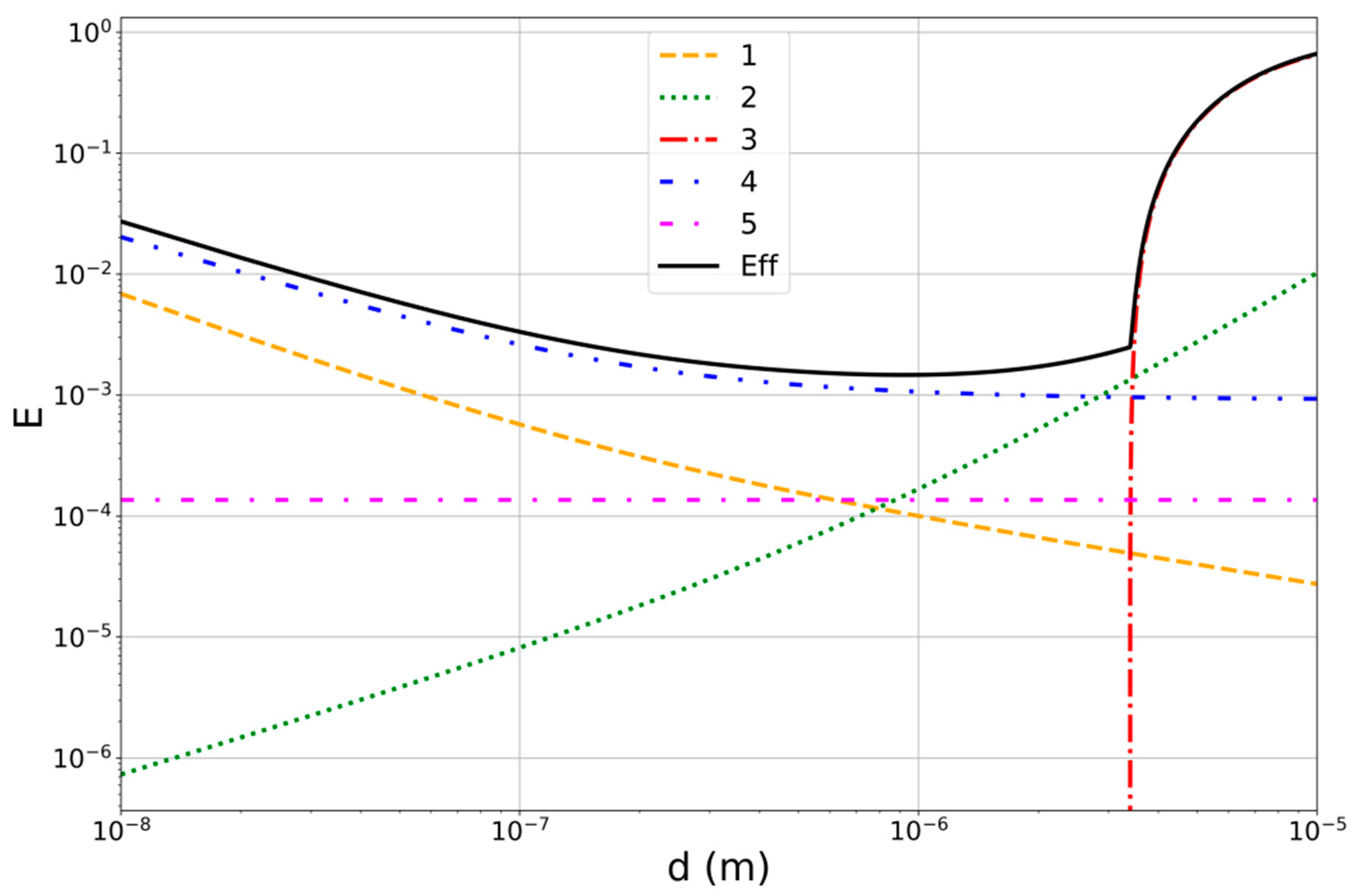
2.1.1. Collision Efficiency E

The collision efficiency E(D, d) is, by definition, the ratio of the actual collision cross section to the geometric cross section of the raindrop. The value E = 1 means that all particles in the geometric volume swept by the falling raindrop will be collected by the raindrop. Usually the values of E << 1 [34].
There are a number of different models for evaluating the collision efficiency. The following models for calculating E were used in this paper to form a multi-model ensemble: the Slinn model [35] (hereinafter the SL83 model); the extended model SL83+ [36], which takes into account the contributions of thermo- and diffusiophoresis; the Pripachkin model [37] (hereinafter PR19).
Figure 1 shows a schematic representation of the contributions of processes that affect the wet deposition for various aerosol particle diameters, built according to the SL83+ model, as well as the contribution of thermo- and diffusiophoresis at a fixed raindrop diameter D = 1 mm and a difference between particle and raindrop absolute temperatures of T a T s = 3 °C. It can be seen that the Brownian diffusion has a greater effect for small particles (with a diameter of less than 0.01 µm), while impaction affects large particles (with a diameter of more than 2 µm). Aerosols in the range of 0.01–2 µm (the so-called Greenfield Gap range) are least scavenged. The contribution of thermophoresis decreases with particle diameter increase. Diffusiophoresis does not depend on the aerosol particle diameter.
Parameterization of collision efficiency of an aerosol particle by a raindrop in the SL_83 model
The SL83 model takes into account the influence of Brownian diffusion processes, impaction, and interception. The collision efficiency E is expressed as [30]:
E ( d , D ) = E B r + E i n t + E i n e
where EBr, Eint, and Eine are the efficiencies of diffusion, interception and inertial impaction, respectively.
E B r = 4 R e D S c ( 1 + 0.4 R e D 1 2 S c 1 3 + 0.16 R e D 1 2 S c 1 2 )
E i n t = 4 d D [ μ a μ w + d D ( 1 + 2 R e D 1 2 ) ]
E i n e = ( S t S t * S t S t * + 2 3 ) 3 / 2
where D and d are the diameters of a raindrop and an aerosol particle, correspondingly, m; S t = 2 τ ( V ( D ) v ( d ) ) D is the Stokes number; V(D) and v(d) are the terminal velocities of raindrops and particles, correspondingly, (v(d) << V(D));  τ = ( ρ p ρ a ) d 2 C c 18 μ a is the relaxation time of particles; μa, μw are the dynamic viscosity of air and water, correspondingly, kg/(m·s); S t * = 1.2 + 1 / 12 ln ( 1 + R e D ) 1 + ln ( 1 + R e D ) is the critical Stokes number calculated for a raindrop; R e D = D · V ( D ) 2 ν is the Reynolds number calculated for a raindrop with a diameter D; S c = μ a ρ a · D d i f f is the Schmidt number calculated for a raindrop; ρa, ρp are the air density and particle density, kg/m3; C c = 1 + 2 λ a d ( 1.257 + 0.4 e 0.55 d λ a ) is the Cunningham correction for aerosol particle glide; λ a = 0.0651 · 10 6 is the mean free path of air molecules, m; D d i f f = C c k b T a 3 π μ d is the diffusion coefficient of aerosol particles in air, m2/s; and k b = 1.38 · 10 23 is the Boltzmann constant, J/K. For particles of mass density ρ p different from 1.0, g/cm3, the inertial contribution to the collision efficiency should be scaled by ( ρ w ρ p ) 1 / 2 [35].
Parameterization of the collision efficiency in the SL_83+ model
The model is based on the SL83 model, which takes into account the models of thermo- and diffusiophoresis processes. The aerosol particle collision efficiency E is as follows:
E ( d , D ) = E B r + E i n t + E i n e + E t h + E d p h  
According to [36], the contributions of thermophoresis Eth and diffusiophoresis Edph to the efficiency E can be expressed as follows (other terms of the sum are similar to the SL83 model):
E t h ( d , D ) = 4 α t h ( 2 + 0.6 R e D 1 2 P r 1 3 ) ( T a T s ) V ( D )   D
E d p h ( d , D ) = 4 β d p h ( 2 + 0.6 R e D 1 2 S c w 1 3 ) ( p s 0 T s p a 0 R H T a ) V ( D )   D
Coefficients αth and βdph are defined by the following expressions, correspondingly:
α t h = 2 C c ( k a + 5 λ a D k p ) k a 5 P ( 1 + 6 λ a D ) ( 2 k a + k p + 10 λ a D k p )
β d p h = T a D d i f f w a t e r P M w M a
where P r = c p μ a k a is the Prandtl number; S c w = μ a ρ a D d i f f w a t e r is the Schmidt number for water vapor in air; D d i f f w a t e r = 0.25·10−4 [38] is the water vapor diffusion coefficient in the air, m2/s; RH is the relative air humidity; P is the normal atmospheric pressure, Pa; Ta is the absolute air temperature, K; Ts is the absolute temperature of the raindrop surface, K (in [18,36,39], the values of Ts and Ta were chosen to obtain T a T s = 3 °C); p s 0   p a 0 is the pressure of water vapor at temperatures T a   T s , Pa; k a ,   k p is the thermal conductivity of air and particles, W/m∙K; M w = 18.0 and M a = 28.97 are the molecular masses of water and air, a.m.u.

2.1.2. Terminal (Falling) Velocity V

The terminal raindrop velocity (raindrop fall velocity) is the terminal vertical component of the raindrop velocity, which is achieved by balancing drag force of the medium with the raindrop gravity.
Table 1 lists the parametrizations of the terminal raindrop velocity, m/s, from [18].
Figure 2 shows the dependence of the calculated terminal velocity on the raindrop diameter for the selected models. One can see that around the raindrop diameters of ~0.1 mm and ~10.0 mm, the terminal velocity values differ by several times for the selected parametrizations, which in turn will affect the results of calculations, if the size distribution of raindrops is taken into account.

2.1.3. Raindrop Size Distribution N(D)

The following raindrop size distributions were chosen for the current study:
Raindrop size distribution ND_MP48
Exponential distribution [40]:
N ( D ) = N 0 e e β e D
where N0e = 0.08∙108 m−4 is the entanglement parameter (at D = 0); D is the raindrop diameter, m; βe = 4100 × I−0.21 m−1 is the slope parameter; I is the rain intensity, mm/hour.
Raindrop size distribution ND_FL86
Lognormal distribution [41]:
N ( D ) = N t o t a l 2 π D   log ( σ D ) exp ( ( log ( D / D g ) ) 2 2 l o g 2 ( σ D ) )
where D is the raindrop diameter, mm; Ntotal is the total raindrop density, m−3; Dg is the raindrop median diameter, mm; σ D is the standard geometric deviation.
σ D * = 1.43 3.10 × 10 4 I
N t o t a l = 172   I 0.22
D g = 0.75   I 0.21
where (*) is used for the variables, for which the approximation is based on the intensity of precipitation I; σ* is only applicable for I > 5 mm/h.

2.1.4. Models for Comparison of Concentration Loss for the Integral Spectrum of Aerosol Particles

Pripachkin microphysical model PR19
In this model, the collision efficiency takes into account the processes of Brownian diffusion, impaction, and the interception of an aerosol particle by a raindrop and does not take into account the thermo-diffusiophoresis and the electrostatic interaction. The raindrops are represented as a system of spherical obstacles that form a homogeneous filtering medium for capturing the aerosol particles [37]. The below-cloud scavenging coefficient Λ is determined by the following expression:
Λ ( d ) = 3 2 E ( d , D ) I 1 D
The aerosol collision efficiency E(d, D) is related to the capture coefficient η, as follows:
E ( d , D ) = 1 e γ η
where γ = 4 α H π D is a coefficient depending on the macroscopic parameters of the medium (~1.0), α = π D 3 n ( D ) 6 is the partial density of raindrops (varies from 10−5 to 10−10 for raindrops with a size of 0.1–6 mm, respectively), n(D) is the volume concentration of raindrops, m−3, H is the vertical size of the reference volume (from 102 to 103 m), η = η s t + η D + η D K are the coefficients of inertial, diffusion capture, and capture due to entanglement, respectively.
η s t = S t S t * S t
η D = 4 × ( 1 + 0.4 R e D 1 2 S c 1 3 ) R e D S c
η D K = 4 r [ μ a μ w + r ( 1 + 2 R e D 1 2 ) ]
where St is the Stokes number calculated for a raindrop,   S t * is the critical Stokes number, Sc is the Schmidt number, R e D is the Reynolds number calculated for a raindrop of diameter D (St, S t * , Sc, R e D μ a , μ w ; see model SL83), and r = d/D is the entanglement parameter.
Parameterized model FLEXPART v10.3
This model was used in the transport code FLEXPART (version v10.3 and higher) to calculate the below-cloud scavenging coefficient [33]; a detailed description of the model is presented in [42].
log ( Λ Λ 0 ) = a + b D p 4 + c D p 3 + d D p 2 + e D p 1 + f ( I I 0 ) 0.5
where Λ0 = 1.0 1/s, I0 = 1.0 mm/h, Dp = log d d 0 , d0 = 1.0 m, a = 274.36, b = 332839.6, c = 226656, d = 58005.9, e = 6588.38, and f = 0.24498.
Integral models of the codes NAME and FLEXPART
These models were used in the transport code NAME [32] and FLEXPART (versions below v10.3; a detailed description is presented in [33]) to calculate the below-cloud scavenging coefficient in the form of dependence of the type Λ = aIb.
NAME Λ = 8.4 × 10 5   I 0.79
FLEXPART Λ = 0.33 × 10 4 I 0.42 + 1.0 × 10 4 I 0.58

2.2. Statistics

The following values were calculated as statistical metrics for selecting the ensemble members: FB—fractional bias, R—Pearson’s correlation coefficient.
F B = x o ¯ x p ¯ 0.5 · ( x o ¯ + x p ¯ )
R = i = 1 n ( x p i x p ¯ ) ( x o i x o ¯ ) i = 1 n ( x p i x p ¯ ) 2 i = 1 n ( x o i x o ¯ ) 2
FAC 5   =   Proportion   of   data   satisfying   0.2   x p x o 5
FAC 10 = Proportion   of   data   satisfying   0.1   x p x o 10
where xp are predicted values, and xo are experimental values.

2.3. Ensemble Verification

The rank histograms (Talagrand diagrams) [43] characterize bias of ensemble estimate and allow demonstrating the reliability of the ensemble forecast in comparison with a sample of experimental data. The interpretation of the rank histogram is based on the assumption that all ensemble members, as well as observation data, have the same distribution. If the ensemble units are chosen in such a way that the observations equally “fit” between the ensemble members, then the rank histogram is flat. The asymmetric type of the histogram indicates a bias of the mean value of the forecasts. If the rank histogram is symmetrical and U-shaped, this means that the ensemble distribution does not cover the observations. If the histogram is Λ-shaped, the distribution is scattered. When the experimental value is less than the ensemble calculations, bin 1 is assigned to it; if the experimental value is in second place in ascending order, bin 2 is assigned to it, etc.

2.4. Experimental Data

The experimental data were taken from the studies of below-cloud scavenging of aerosols by raindrops [35,44,45,46,47]. Unfortunately, at the moment, there is a lack of experimental data on below-cloud scavenging, and in most studies the data are presented in the form of an integral approximation, both in terms of precipitation intensity and disperse composition of aerosols. The data given in the study conducted by Sparmacher were obtained under controlled conditions and are the best in terms of their “validity”. Table 2 presents the experimental values of the below-cloud scavenging coefficient Λ, as well as the conditions under which they were obtained.
The experimental data from experiments 8 and 9 also could be described using the ensemble approach, but the conditions under which such experiments were carried out led to dominance of the in-cloud scavenging process [18]. In this paper, we decided to focus on below-cloud scavenging models only, but we cannot ignore the recent experimental data, so we performed assessments by combining in-cloud and below-cloud scavenging models to ensure that these experimental data can be also covered. For this purpose, models (Jylha’s model [50], Environ’s model [51], Pudykiewicz’s model [52])were taken and applied under experimental conditions.
Jylha   1991 Λ = 3.4 × 10 5 I 0.55
Environ   2018 Λ = 4.2 × 10 4 I 0.79
Pudykiewicz   1989 Λ = 3.5 × 10 5 R H R H 0 R H c R H 0 ,   R H > 80 %
where Λ is an in-cloud scavenging coefficient, 1/s; I is rain intensity, mm/h; RH is relative humidity, %; RH0 is a threshold value of the relative humidity above which the subgrid scale condensation occurs; RHc is a relative humidity for the saturation state. As can be seen in Figure 3, the in-cloud scavenging process determines the scavenging coefficient and deposition rate. Thus, we will focus on the experimental data 1–7 from Table 2, and in further work we will consider the cleaning process in the cloud as a separate process, the models of which, also using the ensemble preparation method studied in this work, will be tested and built in the same way.

3. Results and Discussion

3.1. Set of Below-Cloud Scavenging Models

Based on the collision efficiency models, the terminal raindrop velocity, and the size distribution of raindrops, a set of models (Table 3) of below-cloud scavenging was formed, which was then tested against the experimental data.
The curves in Figure 4 represent all 16 combinations of below-cloud scavenging models calculated using the parameters of experiment Nos. 1 and 2 (Table 2). Integrals for models were calculated by the numerical Simpson’s 1/3 rule.

3.2. Partitioning of the Study Area According to Diameter Ranges

Due to the fact that the values of below-cloud scavenging coefficient Λ differ by several orders of magnitude (from 10−7 to 10−3) depending on the diameter of aerosol particles, the study area was divided into two groups according to the characteristic sizes of aerosol particles: the fine aerosol group: 0.1–1.0 µm; and the coarse group: 1.0–10.0 µm. Figure 5 show the histograms of normalized systematic errors for both groups of diameters. The histogram in Figure 5a shows that for the fine aerosol group, all combinations of models that include the SL83 collision efficiency model underestimate the values of the coefficient Λ, while the models that include the SL83+ model (that takes into account the thermo- and diffusiophoresis in addition to SL83), on the contrary, overestimate them. This is probably related with the limited experimental data in the fine aerosol group. In the coarse group (Figure 5b), the models have both positive and negative FB values, depending on the transition between exponential and lognormal raindrop distribution systems.
Since the choice of parameterization of terminal raindrop fall velocity does not strongly affect the scavenging coefficient, it was decided for ensemble constructing to use the models with different descriptions of collision efficiency, as well as different systems of raindrop distribution, to give an unbiased estimate in total.

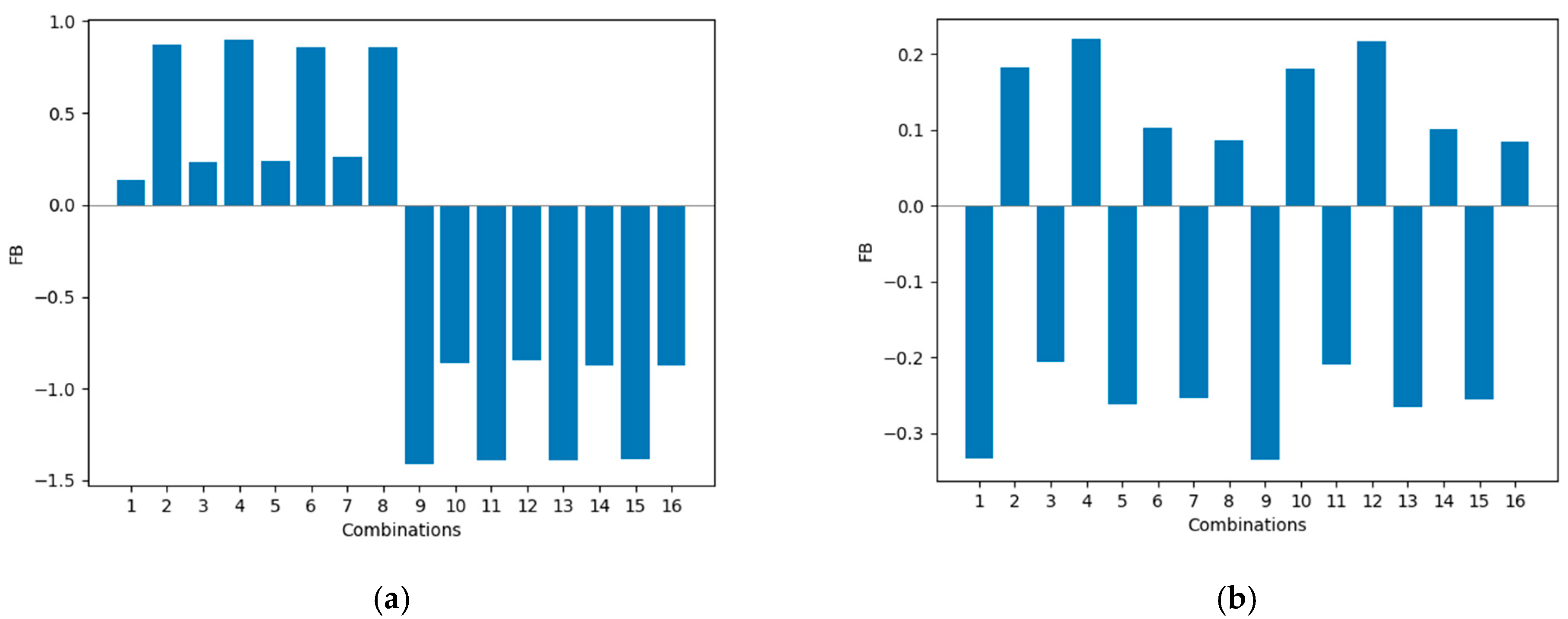
3.3. Results of Calculations of Statistical Metrics

The values of statistical metrics for the constructed set of below-cloud scavenging models are given in Table 4. Pearson correlation coefficient values are about 0.6 for the fine group and about 0.5 for the coarse group; FAC5 values range from 0.28–1.0 for the fine group and are about 0.5 for the coarse group; FAC10 values range from 0.64–1.0 for the fine group and are approximately 0.7 for the coarse group. The results indicate that the used set of disperse models is valid in terms of reproducing experimental data both for fine and coarse aerosol fractions. Further construction of a multi-model ensemble involves the enumeration of possible combinations from the selected set that satisfies the criteria of unbiased estimates and compliance of dispersion of the ensemble with dispersion of experimental data. This is done using the rank histograms.

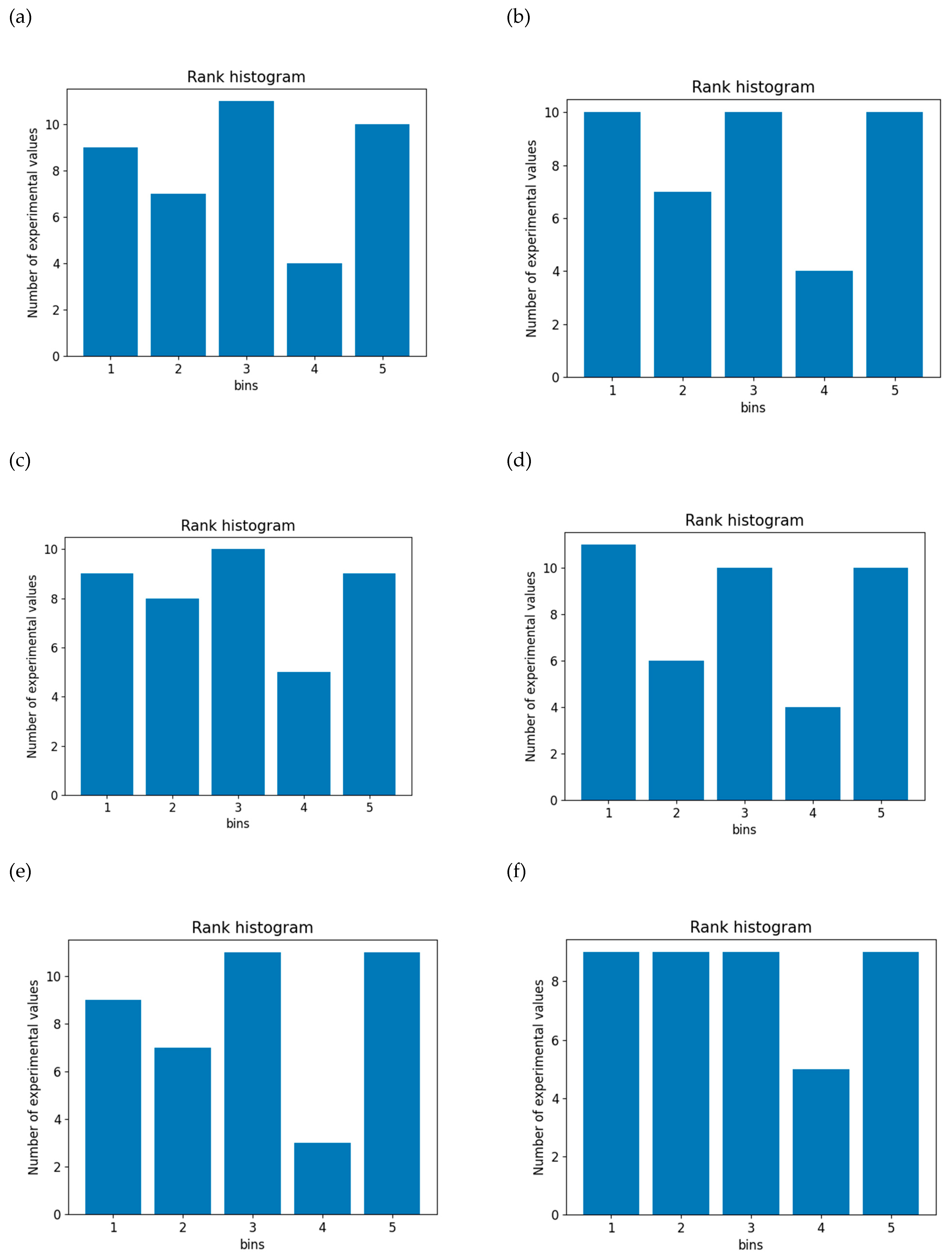
3.4. Construction of Rank Histograms

The applicability of a set of models as an ensemble can be demonstrated by rank histogram. For this task, combinations of models with different collision efficiency descriptions (SL83 and SL83+) as well as different raindrop distribution systems (MP48 and FL86) were taken. A total of 225 combinations, collected from a set of models from Table 3, were analyzed. Rank histograms were used to analyze how the models describe the statistical dispersion of observed values for all experimental data from Table 2. Given the small amount of experimental data, a four-member ensemble was chosen. A larger set, as the calculations showed, led to a strong nonuniformity in the histograms for individual members. Therefore, histograms were constructed for each combination (for each measurement in each experiment, taking into account the conditions, the values of below-cloud scavenging coefficients Λ were calculated for the selected models, they were ranked, and the rank corresponding to the experimental value was determined; the number of experimental values that fell into the corresponding ranks is represented as the column height in the rank histogram).
Examples of the rank histograms for combinations of models are shown in Figure 6a–f. The remaining combinations show a similar behavior in terms of distribution; therefore, they are not presented in this paper. We can conclude that the ensemble with models 1, 4, 13, and 14 in Figure 6f is the best. It can be seen that all experimental values are evenly distributed among the ensemble members, which indicates that the estimate of the multi-model ensemble is unbiased. A similar behavior was observed in the analysis of meteorological ensemble in [16], where many more experimental points are available; nevertheless, there are also bins with behavior that is not ideal with respect to the overall distribution. The constructed ensemble has an unbiased estimate. If we consider the ensemble by all measurements, then the average characteristics are FB~−0.3, Pearson~0.6, FAC5~0.7, and FAC10~0.9 for the fine group, and FB~0.1, Pearson~0.5, FAC5~0.6, and FAC10~0.7 for the coarse group, which is acceptable considering a wide range of Λ. We shall consider further the results of calculations for this ensemble based on experimental data separately for each experiment, integrating the spectrum of aerosol particles over diameters for the postulated form of size distribution of aerosol particles.

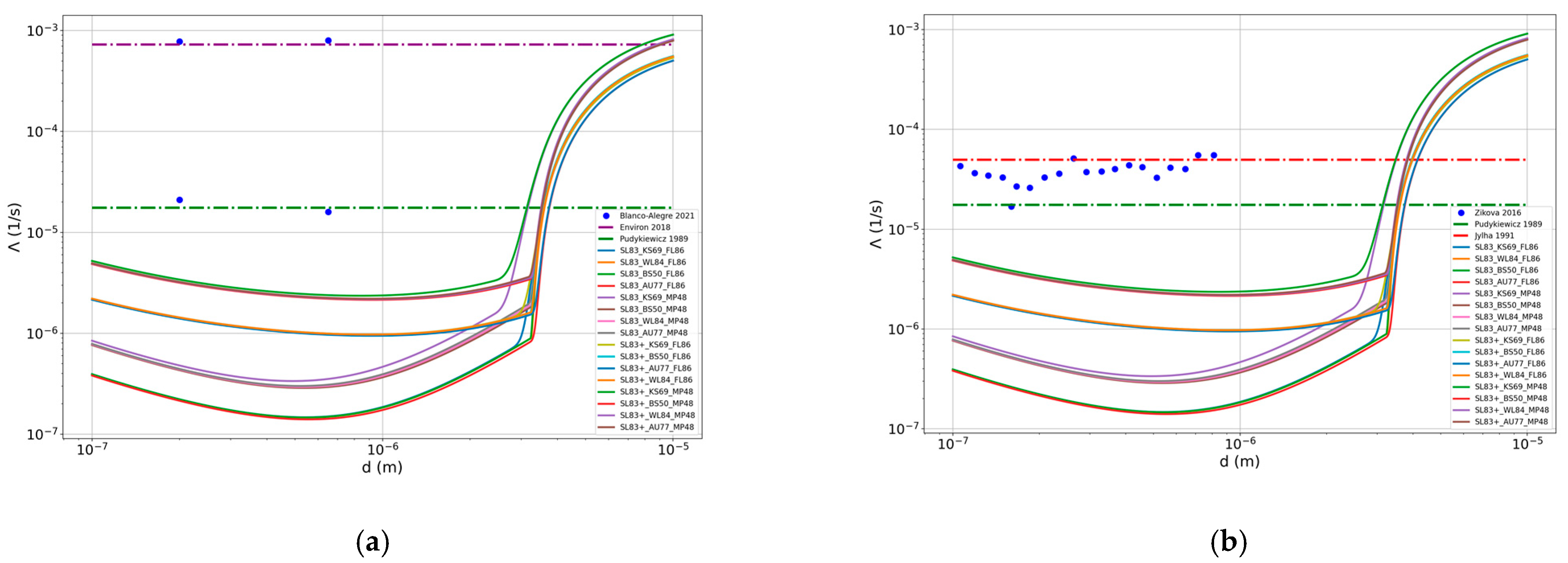
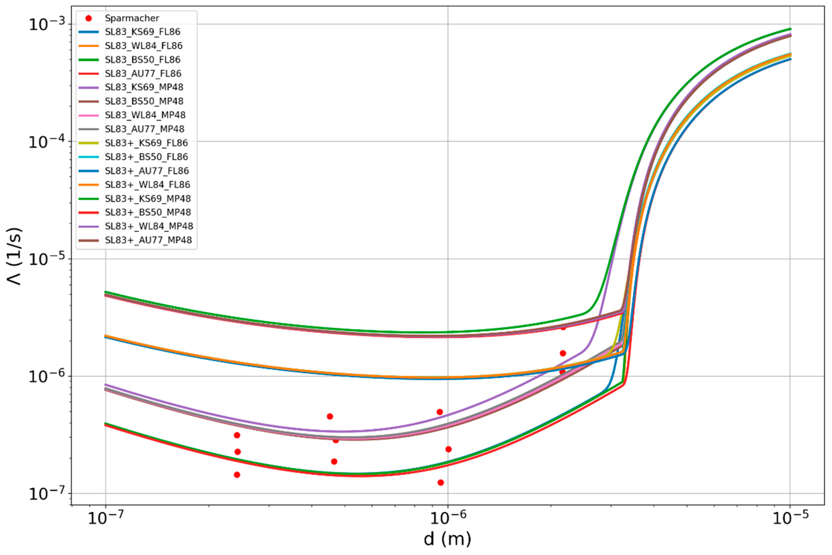
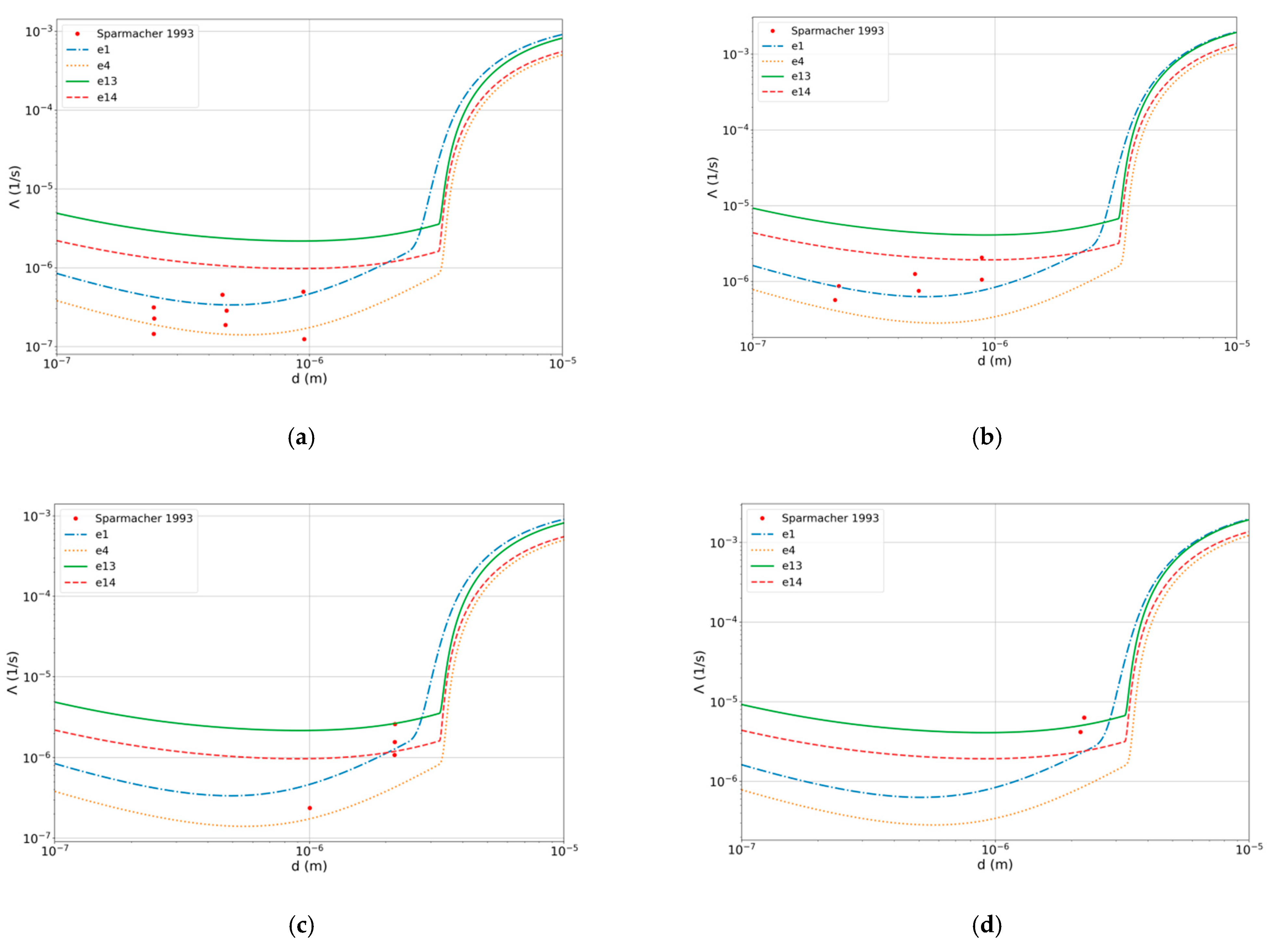
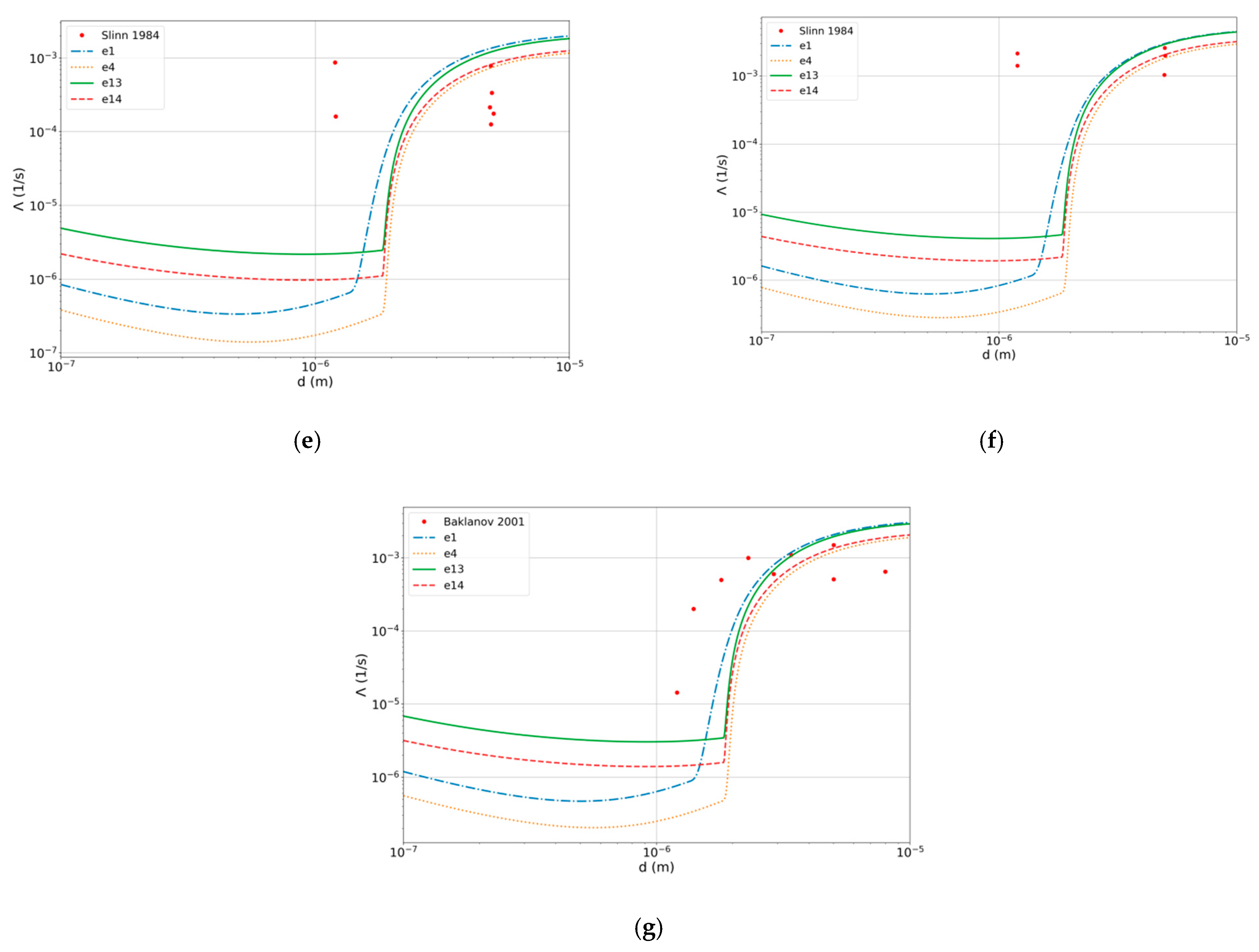
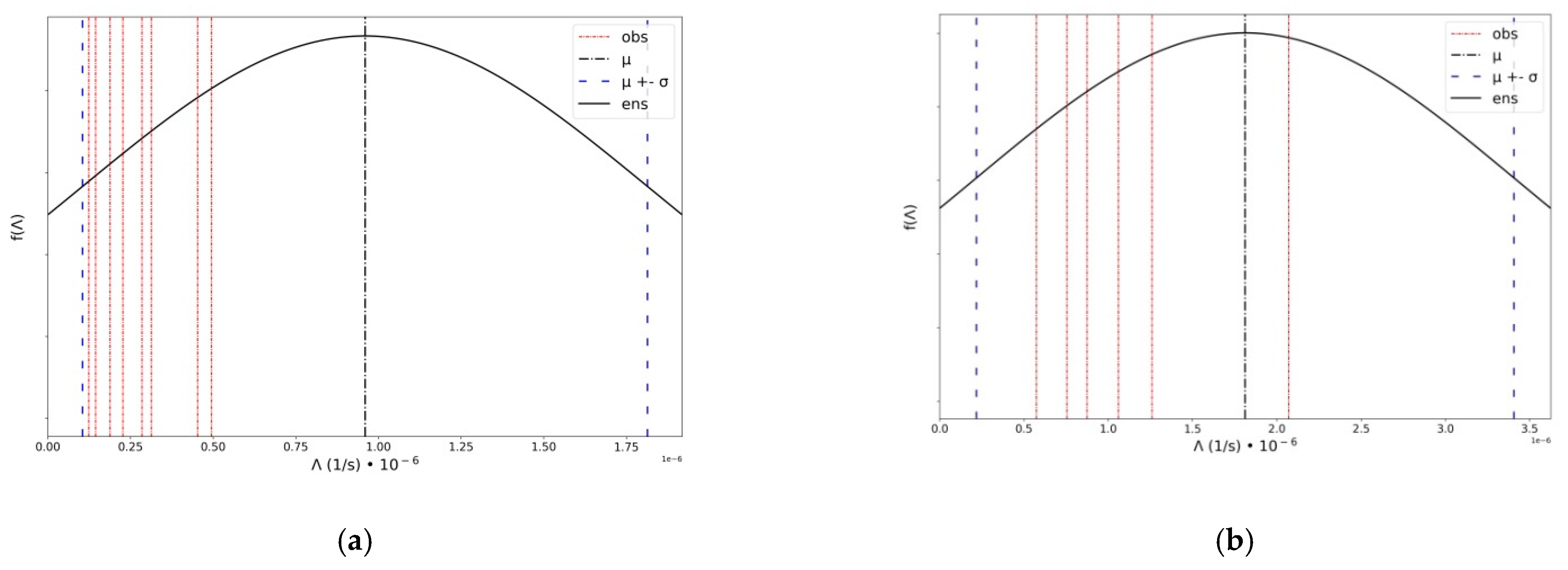
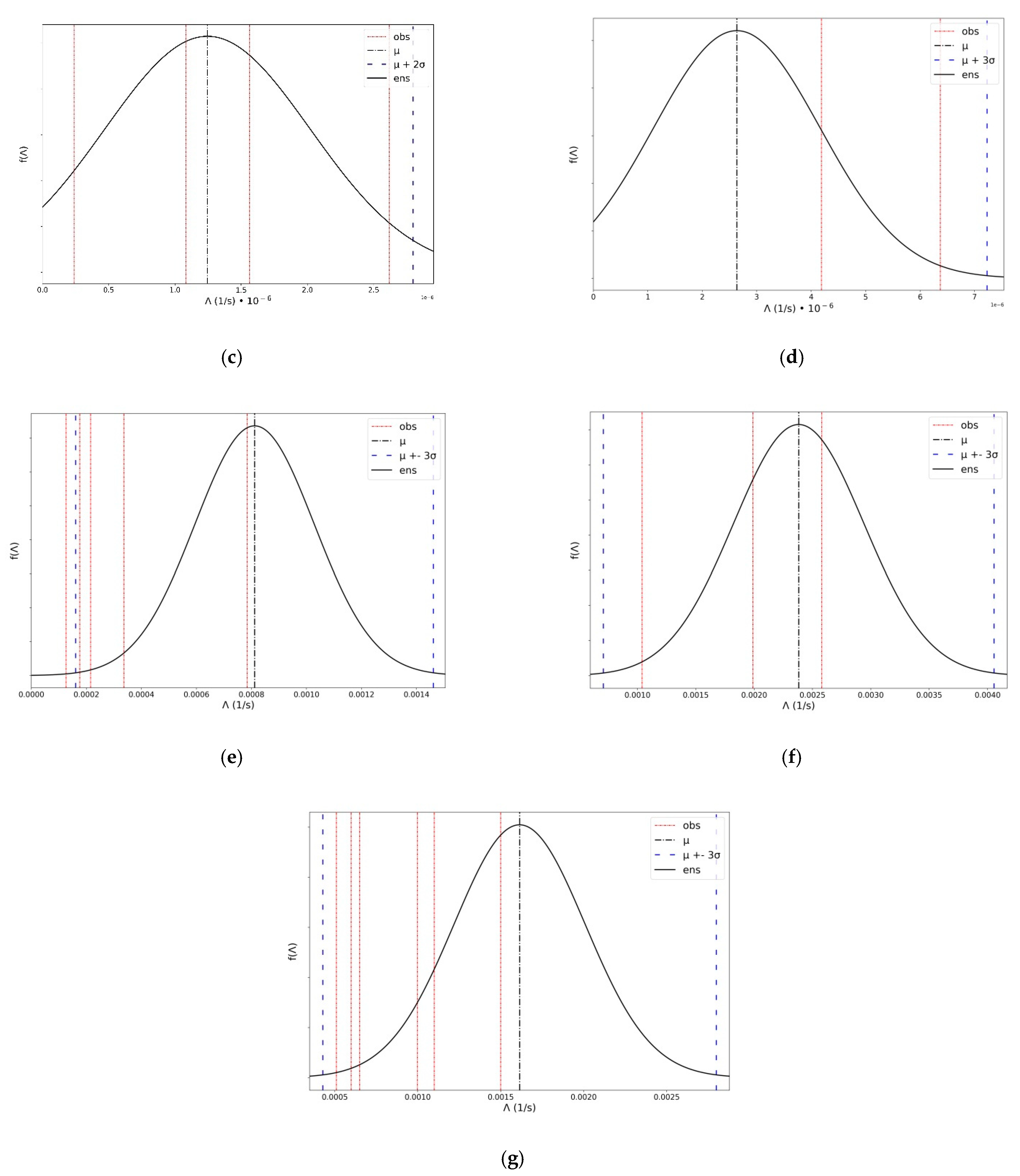
3.5. Comparison of the Results of Model Calculations for the Ensemble with Experimental Data

To estimate the statistical dispersion of the ensemble with respect to the experimental data, we used an approach based on the approximation of the results of ensemble calculation by the normal distribution function. For this purpose:
  • Groups of diameters were selected in the experimental data, for which the scavenging value was within the error of the experimental data. This was used to separate the coarse areas from the fine areas;
  • Model calculations of the below-cloud scavenging coefficient Λ were carried out for the average diameter of an aerosol particle d ¯ corresponding to the experiment in the considered group of diameters;
  • Then, using the obtained values, the average value μ = i = 1 4 Λ ( d ¯ ) i 4 and standard deviation σ = i = 1 4 Λ ( d ¯ ) i 2 4 ( i = 1 4 Λ ( d ¯ ) i 4 ) 2 was calculated;
  • The fractions of the experimental values that fall into the ranges μ ± σ ,     μ ± 2 σ , and μ ± 3 σ were analyzed.
Figure 7a–g shows the results of the model calculations for the ensemble (curves e1, e4, e13, and e14) in comparison with the experimental data from Table 2. Figure 8a–g shows the resulting distribution densities of the ensemble (curve ens) together with the experimental results from Table 2. One can see from the figures that the ensemble distributions cover 100% of experimental data Nos. 1, 2 within σ (Figure 8a,b), 100% of experimental data No. 3 within 2σ (Figure 8c), and 80–100% of experimental data Nos. 4–7 within 3σ (Figure 8d–g).

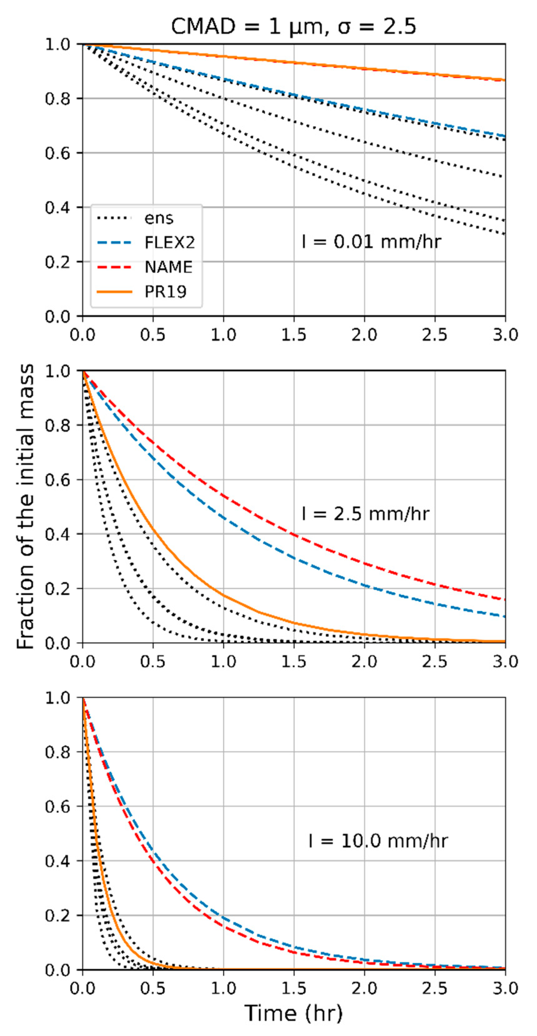
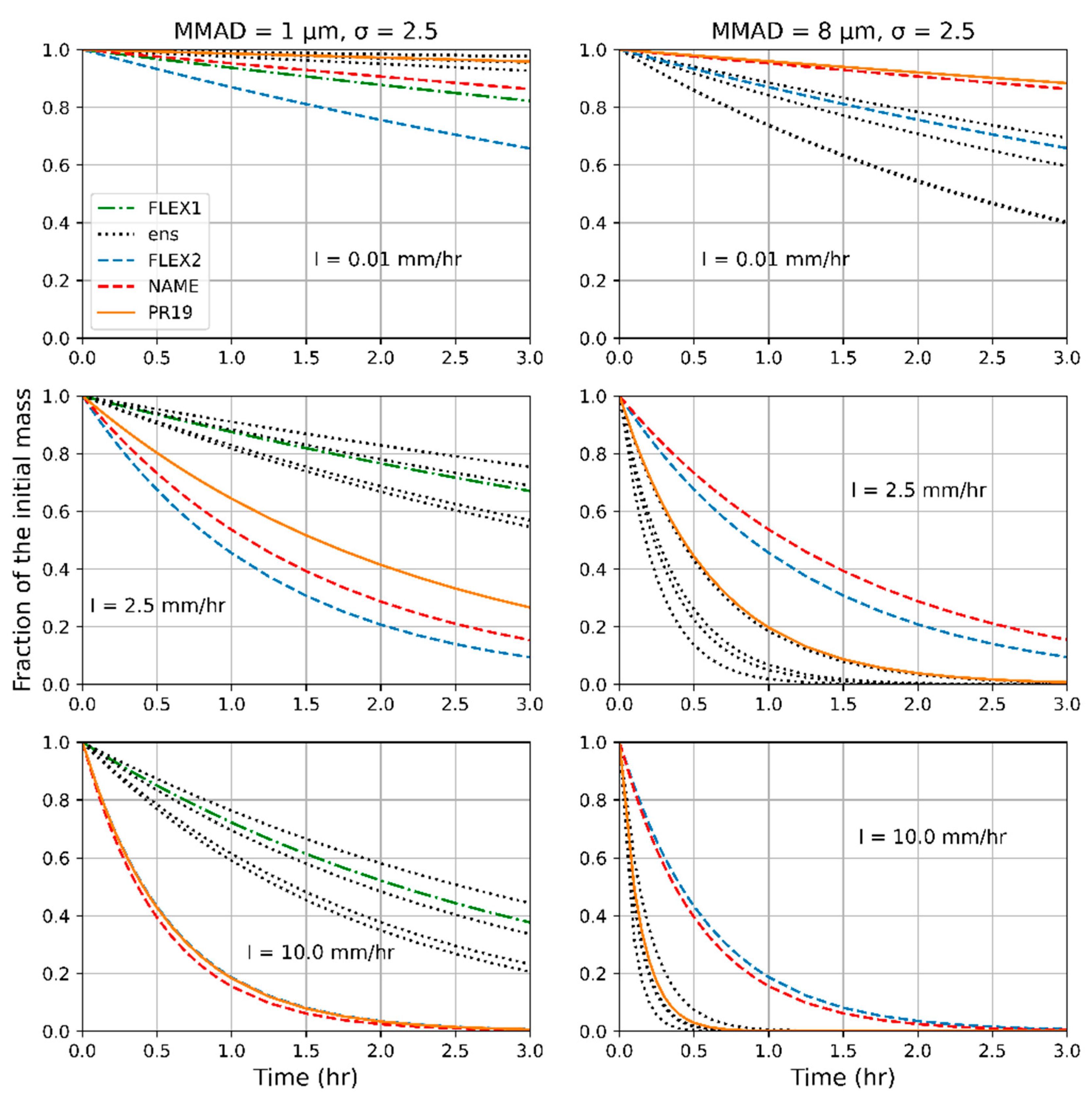
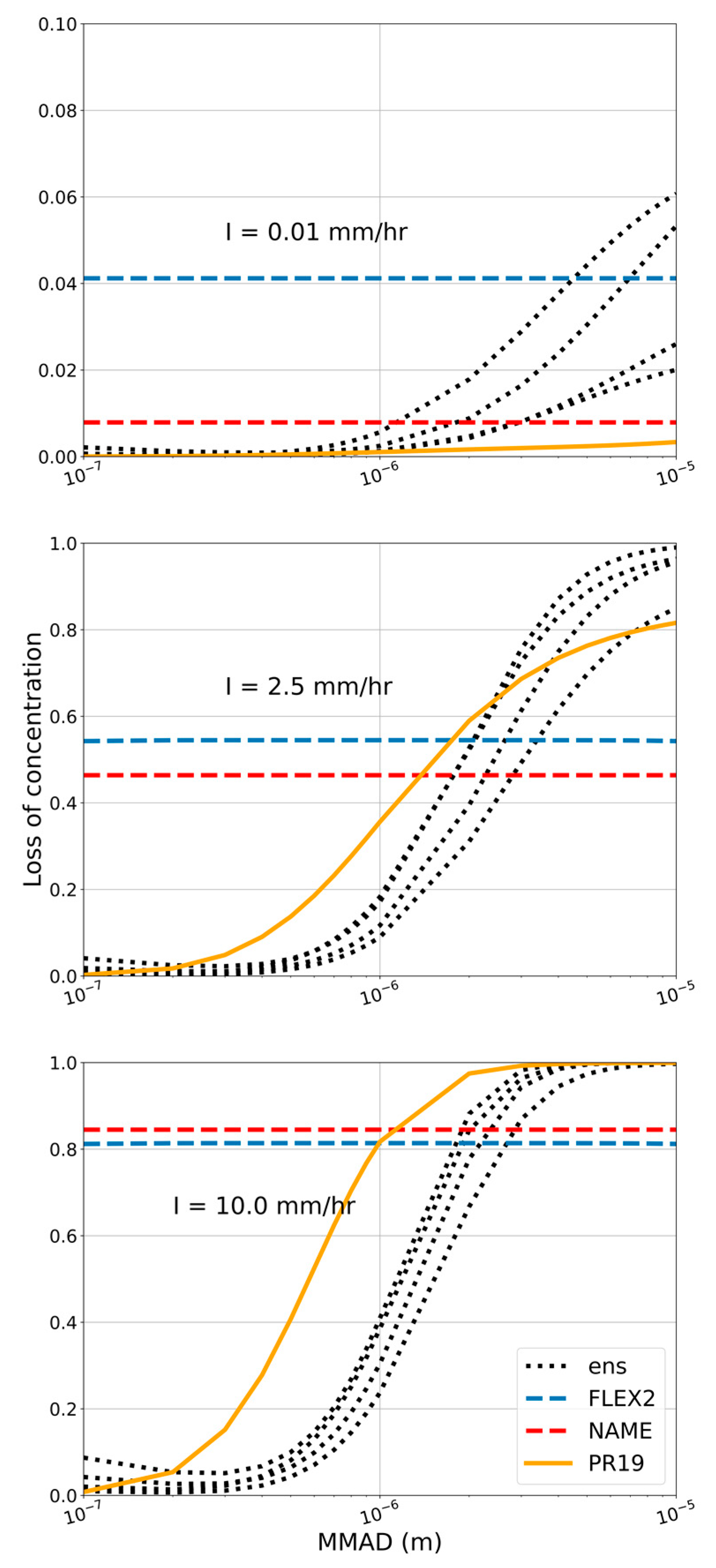
3.6. Calculation of Polydisperse Aerosol Scavenging from a Control Volume

In this section, we analyze how the choice of below-cloud scavenging model affects the results of estimates of changes in the concentration of aerosol particles in the test volume due to scavenging. The models described in Section 2.1.4, and the used multi-model ensemble were studied for this analysis.
First, the lognormal aerosol size distribution with different CMAD (count median aerodynamic diameter) and σ = 2.5 was considered; the scavenging time was varied between 0 to 3 h. This test was conducted to compare results integrated over droplet and particle size distributions in comparison with previous studies. The FLEXPART integral model was not tested here due to limitation of 500 nm in maximum particle size. The CMAD of 1 µm corresponds to an MMAD (mass median aerodynamic diameter) of about 12.4 µm (for 4000 kg/m3 density), and a major part of the mass is concentrated in the range exceeding the model applicability.
As can be seen from Figure 9 for CMAD = 1 µm for precipitation intensities of 2.5 and 10 mm/h, the results of calculations using ensemble models are close to the Pripachkin model. For lower intensities, the results are in good agreement with the FLEXPART integral model. With the increase of precipitation, the intensity difference becomes significant and reaches the values of 0.2–0.5; the results obtained using ensemble models are higher than those calculated by the Pripachkin model. The other models considered significantly overestimate fraction of mass concentration in comparison with the ensemble models (underestimation of deposited values). The same behavior of mass concentration in the control volume could be found in studies [18,53].
The next set of results is devoted to the analysis of the characteristic distributions of pollutant emissions into the atmosphere. The lognormal distribution with different MMAD and σ = 2.5 was considered as the aerosol size distribution; the scavenging time was varied from 0 up to 3 h. Since the actual diameter is used in the below-cloud scavenging models for Λ calculations, the aerodynamic diameter of aerosol spectrum was recalculated according to d = d a /   ρ a ρ 0 , where da is the aerodynamic diameter and ρ 0 = 1000 kg/m3. Two cases were studied. In the first case, the dependence of concentration fraction in control volume on the timing of precipitations was studied. Values of 1.0 μm [54] and 8 μm [55] were taken as the MMAD (of the lognormal aerosol distributions representative of accidental releases). It was seen (Figure 10) that for low intensities, the results of calculation of concentration loss are in good agreement with each other. For an MMAD of 1 µm, the FLEXPART parameterized dispersion model gives values within the ensemble distribution, and the FLEXPART curve is close to ensemble mean. For MMADs of 1 μm and 8 μm, the integral models give underestimated and overestimated results of concentration loss in the control volume. In all cases, the ensemble covers at least one of the integral models, which corresponds to ensemble forming objectives.
In the second case, the dependence of the fraction of scavenging concentration on the MMAD of the lognormal aerosol distribution was studied; the precipitation intensity I was taken equal to 0.01, 2.5, and 10 mm/h, and the duration of precipitations was set to 1 h.
Figure 11 shows that the concentration loss increases with increasing MMAD for models that take into account the dispersed structure of aerosols. At a value of MMAD ~10−5 m, the proportion of the washed out concentration tends toward 100% at high values of precipitation intensity.
For lower values of intensity, the ensemble gives reasonable dispersion up to 160% from the results averaged over ensemble members. The spread of the results decreases with the MMAD’s increase: for 0.01 mm/h, from 240% to 100%; for 2.5 mm/h, from 200% to 14%; for 10 mm/h, from 200% to 0.2%. The curves intersect the FLEXPART integral model, the NAME integral model, and the Pripachkin model in the MMAD range between 10−6 and 10−5. In general, there is an overestimation of washed out concentration when using integral models compared with the results based on the models that resolve the spectrum of aerosol particles for aerosols with MMAD of 2 µm or less, and an underestimation for coarse ones. In addition, after integration over the spectrum of aerosol particles, a decrease in dispersion of the ensemble is seen. However, it should be noted that the source of release can also be practically monodisperse (for example, a filtered release [56] or the release of molecular forms of radionuclides [57]).

4. Conclusions

The paper presents the results of a multi-model ensemble construction to determine the below-cloud scavenging coefficient in atmospheric transport models. Combinations of models describing the efficiency of aerosol capture by raindrops, the terminal raindrop fall velocity, and the size distribution of raindrops were considered as members of the ensemble. The following criteria for constructing a multi-model ensemble were used: the unbiased estimate, characterized by a flat form of a rank histogram, as well as ensemble dispersion of no more than 3σ of the normal distribution covering the statistical spread of experimental data. As a result of the study, it was found that the following combinations of models satisfy these requirements: the Slinn 83 collision efficiency model with the Kessler 1969 raindrop velocity model and exponential raindrop size distribution, as well as with the Atlas 1977 model and lognormal distribution. In addition, the modified Slinn 83 model, which takes into account the processes of thermo- and diffusiophoresis, was included in the constructed ensemble in combination with the Willis 1984 model using both exponential and lognormal raindrop size distributions. The following range of metric values as a result of comparison with experimental data is found: FB (−1.4–0.9), FAC10 (0.64–1.0), Pearson (~0.6) for the fine fraction and FB (−0.3–0.2), FAC10 (~0.7), and Pearson (~0.5) for the coarse fraction.
Based on experimental data in two ranges of particle diameters, using the ensemble approximation by a normal distribution, the FB metric, and Talagrand rank diagrams, it was found that the constructed ensemble provides an unbiased estimate. Perhaps, when using an ensemble in an atmospheric dispersion model, it is worth using this ensemble to reproduce the statistical characteristics of the normal distribution and then use the Monte Carlo method in the complex ensemble forecast. The results were compared with integrated models (not taking into account the size spectrum of aerosol). It was found that the ensemble forecast is physically adequate; the integral models tend to overestimate the concentration decrease (increase in predicted deposition) in the range of fine fractions (up to 1–5 μm) and underestimate the results for coarse fractions. The spread of the ensemble after integration over the spectra of raindrops and aerosol particles decreased to 250%, which decreases with MMAD increase to 100% for low intensities and from 200% to 0.2% for high precipitation rates. Nevertheless, taking into account the different characteristics of aerosols released into the atmosphere due to dispersion and dust suppression, the authors believe it correct to include the advanced approaches that take into account the size characteristics of raindrops and aerosols in the atmospheric transport model. In the future, the authors consider it expedient to develop this approach in describing in-cloud scavenging, which in some cases can also affect estimates of wet deposition.

Author Contributions

Conceptualization, A.K.; methodology, A.K.; validation, A.K., A.O. and V.S.; formal analysis, A.K., A.S. and V.S.; investigation, A.K., A.O. and A.S.; writing—original draft preparation, A.K., A.O., A.S. and V.S.; writing—review and editing, A.K., A.O., A.S. and V.S.; visualization, A.O.; supervision, A.K. All authors have read and agreed to the published version of the manuscript.

Funding

The APC was funded by Nuclear Safety Institute of the Russian Academy of Sciences (IBRAE RAN).

Informed Consent Statement

Not applicable.

Data Availability Statement

Data sharing not applicable.

Conflicts of Interest

The authors declare no conflict of interest.

Nomenclature

µ, μwDynamic viscosity of air and water, kg/m·s
C(d)Concentration of aerosol particles with diameter d, 1/m3
CcCunningham correction for aerosol particle glide
DDiameter of a raindrop, m
dDiameter of a particle, m
DdiffDiffusion coefficient of aerosol particles in air, m2/s
Ddiff waterWater vapor diffusion coefficient in the air, m2/s
E(D)Aerosol particle collision efficiency
EBrEfficiency of Brownian diffusion
EineEfficiency of inertial impaction
EintEfficiency of interception
EdphEfficiency of diffusiophoresis
EthEfficiency of thermophoresis
HVertical size of the reference volume (from 102 to 103 m)
IRain intensity, mm/hour
ka, kpThermal conductivity of air, particles, W/m∙K
kbBoltzmann constant, J/K
Mw, MaMolecular masses of water and air, a.m.u.
N(D)Raindrop size distribution, m−4
n(d)Volume concentration of raindrops, m−3
PNormal atmospheric pressure, Pa
p s 0   p a 0 Pressure of water vapor at temperatures T a   T s , Pa
PrPrandtl number
rEntanglement parameter
ReDReynolds number calculated for a raindrop with a diameter D
ScSchmidt number
ScwSchmidt number for water vapor in air
StStokes number
St*Critical Stokes number
tInteraction time of precipitation and aerosol, s
Ta, TsAbsolute air temperature and absolute temperature of the raindrop surface, K
V(D)Raindrop terminal velocity, m/s
v(d)Particle velocity, m/s
αPartial density of raindrops (varies from 10−5 to 10−10 for raindrops with a size of 0.1–6 mm, respectively)
γCoefficient depending on the macroscopic parameters of the medium (~1.0)
ηCoefficients of inertial diffusion capture and capture due to entanglement
ΛBelow-cloud scavenging coefficient, 1/s
λaRean free path of air molecules, m
νRinematic viscosity, m2/s
ρa, ρpRir density, particle density, kg/m3
τRelaxation time of particles, s

References

  1. International Atomic Energy Agency. Dispersion of Radioactive Material in Air and Water and Consideration of Population Distribution in Site Evaluation for Nuclear Power Plants; Safety Standards Series No. NS-G-3.2; International Atomic Energy Agency: Vienna, Austria, 2002. [Google Scholar]
  2. International Atomic Energy Agency. Operations Manual for IAEA Assessment and Prognosis During a Nuclear or Radiological Emergency; Emergency Preparedness and Response; IAEA: Vienna, Austria, 2020. [Google Scholar]
  3. Wang, Y.; Schmid, F.; Harou, A. Guidelines for Nowcasting Techniques; World Meteorological Organization: Geneva, Switzerland, 2017; ISBN 978-92-63-11198-2. [Google Scholar]
  4. Chen, X.; Wang, M.; Wang, S.; Chen, Y.; Wang, R.; Zhao, C.; Hu, X. Weather Radar Nowcasting for Extreme Precipitation Prediction Based on the Temporal and Spatial Generative Adversarial Network. Atmosphere 2022, 13, 1291. [Google Scholar] [CrossRef]
  5. Leadbetter, S.J.; Jones, A.R.; Hort, M.C. Assessing the value meteorological ensembles add to dispersion modelling using hypothetical releases. Atmos. Chem. Phys. 2022, 22, 577–596. [Google Scholar] [CrossRef]
  6. Bakin, R.I.; Gubenko, I.; Dolganov, K.; Ignatov, R.; Ilichev, E.; Kiselev, A.; Krasnoperov, S.; Konyaev, P.; Rubinshtein, K.; Tomashchik, D. Application of ensemble method to predict radiation doses from a radioactive release during hypothetical severe accidents at Russian NPP. J. Nucl. Sci. Technol. 2020, 58, 635–650. [Google Scholar] [CrossRef]
  7. Elahi, E.; Khalid, Z.; Tauni, M.Z.; Zhang, H.; Lirong, X. Extreme weather events risk to crop-production and the adaptation of innovative management strategies to mitigate the risk: A retrospective survey of rural Punjab, Pakistan. Technovation 2022, 117, 102255. [Google Scholar] [CrossRef]
  8. Abid, M.; Scheffran, J.; Schneider, U.A.; Elahi, E. Farmer Perceptions of Climate Change, Observed Trends and Adaptation of Agriculture in Pakistan. Environ. Manag. 2019, 63, 110–123. [Google Scholar] [CrossRef] [PubMed]
  9. COST ES1006; Best Practice Guidelines. COST Action ES1006. University of Hamburg: Hamburg, Germany, 2015.
  10. Hegarty, J.; Draxler, R.R.; Stein, A.F.; Brioude, J.; Mountain, M.; Eluszkiewicz, J.; Nehrkorn, T.; Ngan, F.; Andrews, A. Evaluation of Lagrangian Particle Dispersion Models with Measurements from Controlled Tracer Releases. J. Appl. Meteorol. Climatol. 2013, 52, 2623–2637. [Google Scholar] [CrossRef]
  11. Olesen, H.R. User’s Guide to the Model Validation Kit; Research Notes from NERI no. 226; National Environmental Research Institute: Roskilde, Denmark, 2005; p. 72. Available online: http://research-notes.dmu.dk (accessed on 26 January 2023).
  12. Khan, T.R.; Perlinger, J.A. Evaluation of five dry particle deposition parameterizations for incorporation into atmospheric transport models. Geosci. Model Dev. 2017, 10, 3861–3888. [Google Scholar] [CrossRef] [Green Version]
  13. Saylor, R.D.; Baker, B.D.; Lee, P.; Tong, D.; Li, P.; Hicks, B.B. The particle dry deposition component of total deposition from air quality models: Right, wrong or uncertain? Tellus B Chem. Phys. Meteorol. 2019, 71, 1550324. [Google Scholar] [CrossRef] [Green Version]
  14. Wesely, M.L.; Hicks, B.B. A Review of The Current Status of Knowledge on Dry Deposition. Atmos. Environ. 2000, 34, 2261–2282. [Google Scholar] [CrossRef]
  15. Mun, C.; Cantrel, L.; Madic, C. A Literature Review on Ruthenium Behaviour in Nuclear Power Plant Severe Accidents. Nucl. Technol. 2007, 156, 332–346. [Google Scholar] [CrossRef]
  16. Paesler-Sauer, J. Comparative Calculations and Validation Studies with Atmospheric Dispersion Models; Kernforschungszentrum Karlsruhe: Karlsruhe, Germany, 1986. [Google Scholar]
  17. Sportisse, B. A review of parameterizations for modelling dry deposition and scavenging of radionuclides. Atmos. Environ. 2007, 41, 2683–2698. [Google Scholar] [CrossRef]
  18. Wang, X.; Zhang, L.; Moran, M.D. Uncertainty assessment of current size-resolved parameterizations for below-cloud particle scavenging by rain. Atmos. Chem. Phys. 2010, 10, 5685–5705. [Google Scholar] [CrossRef] [Green Version]
  19. Monin, A.S.; Obukhov, A.M. The main regularities of turbulent mixing in the surface layer of the atmosphere. Proc. Geophys. Inst. Acad. Sci. USSR 1954, 151, 163–187. (In Russian) [Google Scholar]
  20. Piskunov, V.N. Parameterization of Aerosol Dry Deposition Velocities onto Smooth and Rough Surfaces. J. Aerosol Sci. 2009, 40, 664–679. [Google Scholar] [CrossRef]
  21. Fang, S.; Zhuang, S.; Goto, D.; Hu, X.; Sheng, L.; Huang, S. Coupled modeling of in- and below-cloud wet deposition for atmospheric 137Cs transport following the Fukushima Daiichi accident using WRF-Chem: A self-consistent evaluation of 25 scheme combinations. Environ. Int. 2022, 158, 106882. [Google Scholar] [CrossRef]
  22. Ulimoen, M.; Berge, E.; Klein, H.; Salbu, B.; Lind, O.C. Comparing model skills for deterministic versus ensemble dispersion modelling: The Fukushima Daiichi NPP accident as a case study. Sci. Total Environ. 2022, 806, 150128. [Google Scholar] [CrossRef]
  23. Leadbetter, S.J.; Andronopoulos, S.; Bedwell, P.; Chevalier-Jabet, K.; Geertsema, G.; Gering, F.; Hamburger, T.; Jones, A.; Klein, H.; Korsakissok, I.; et al. Ranking uncertainties in atmospheric dispersion modelling following the accidental release of radioactive material. Radioprotection 2020, 55, S51–S55. [Google Scholar] [CrossRef]
  24. Galmarinia, S.; Bianconi, R.; Klug, W.; Mikkelsen, T.; Addis, R.; Andronopoulos, S.; Astrup, P.; Baklanov, A.; Bartniki, J.; Bartzis, J.C.; et al. Ensemble dispersion forecasting—Part I: Concept, approach and indicators. Atmos. Environ. 2004, 38, 4607–4617. [Google Scholar] [CrossRef]
  25. Sorensen, J.H.; Amstrup, B.; Feddersen, H.; Bartnicki, J.; Klein, H.; Simonsen, M.; Lauritzen, B.; Cordt Hoe, S.; Israelson, C.; Lindgren, J. Fukushima Accident: UNcertainty of Atmospheric Dispersion Modelling (FAUNA); NKS Secretariat: Roskilde, Denmark, 2016; p. 43. ISBN 978-87-7893-421-5. [Google Scholar]
  26. Straume, A.G.; Koffi, E.N.; Nodop, K. Dispersion Modeling Using Ensemble Forecasts Compared to ETEX Measurements. J. Appl. Meteorol. 1998, 37, 1444–1456. [Google Scholar] [CrossRef]
  27. Perillat, R.; Korsakissok, I.; Mallet, V.; Mathieu, A.; Sekiyama, T.; Kajino, M.; Adachi, K.; Igarashi, Y.; Didier, D. Using meteorological ensembles for atmospheric dispersion modelling of the Fukushima nuclear accident. In Proceedings of the 18th International Conference on Harmonisation within Atmospheric Dispersion Modelling for Regulatory Purposes, Bologna, Italy, 9–12 October 2017. [Google Scholar]
  28. Kajino, M.; Sekiyama, T.T.; Mathieu, A.; Korsakissok, I.; Périllat, R.; Quélo, D.; Quérel, A.; Saunier, O.; Adachi, K.; Girard, S.; et al. Lessons learned from atmospheric modeling studies after the Fukushima nuclear accident: Ensemble simulations, data assimilation, elemental process modeling, and inverse modeling. Geochem. J. 2018, 52, 85–101. [Google Scholar] [CrossRef] [Green Version]
  29. Kajino, M.; Sekiyama, T.T.; Igarashi, Y.; Katata, G.; Sawada, M.; Adachi, K.; Zaizen, Y.; Tsuruta, H.; Nakajima, T. Deposition and dispersion of radio-cesium released due to the Fukushima nuclear accident: Sensitivity to meteorological models and physical modules. J. Geophys. Res. Atmos. 2019, 124, 1823–1845. [Google Scholar] [CrossRef]
  30. Yegnan, A.; Williamson, D.G.; Graettinger, A.J. Uncertainty analysis in air dispersion modeling. Environ. Model. Softw. 2002, 17, 639–649. [Google Scholar] [CrossRef]
  31. Mandal, S.; Madhipatla, K.K.; Guttikunda, S.; Kloog, I.; Prabhakaran, D.; Schwartz, J.D. GeoHealth Hub India Team, Ensemble averaging based assessment of spatiotemporal variations in ambient PM2.5 concentrations over Delhi, India, during 2010–2016. Atmos. Environ. 2020, 224, 117309. [Google Scholar] [CrossRef] [PubMed]
  32. Webster, H.; Thomson, D. The NAME wet deposition scheme Forecasting Research. Tech. Rep. 2014, 584, 41. [Google Scholar]
  33. Pisso, I.; Sollum, E.; Grythe, H.; Kristiansen, N.I.; Cassiani, M.; Eckhardt, S.; Arnold, D.; Morton, D.; Thompson, R.L.; Zwaaftink, C.D.G.; et al. The Lagrangian particle dispersion model FLEXPART version 10.4. Geosci. Model Dev. 2019, 12, 4955–4997. [Google Scholar] [CrossRef] [Green Version]
  34. Seinfeld, J.H.; Pandis, S.N. Atmospheric Chemistry and Physics: From Air Pollution to Climate Change, 2nd ed.; John Wiley & Sons, Inc.: Hoboken, NJ, USA, 2006; pp. 900–929. [Google Scholar]
  35. Slinn, W.G.N. Precipitation scavenging. In Atmospheric Sciences and Power Production—1979, Chap. 11; Division of Biomedical Environmental Research, U.S. Department of Energy: Washington, DC, USA, 1983. [Google Scholar]
  36. Andronache, C.; Grönholm, T.; Laakso, L.; Phillips, V.; Venäläinen, A. Scavenging of ultrafine particles by rainfall at a boreal site: Observations and model estimations. Atmos. Chem. Phys. 2006, 6, 4739–4754. [Google Scholar] [CrossRef] [Green Version]
  37. Pripachkin, D.A.; Budyka, A.K. Influence of the parameters of aerosol particles on their scavenging from the atmosphere by raindrops, Izvestiya RAN. Phys. Atmos. Ocean. 2020, 56, 203–209. (In Russian) [Google Scholar]
  38. Montgomery, R.B. Viscosity And Thermal Conductivity Of Air And Diffusivity Of Water Vapor In Air. J. Atmos. Sci. 1947, 4, 193–196. [Google Scholar] [CrossRef]
  39. Bae, S.Y.; Jung, C.H.; Kim, Y.P. Relative contributions of individual phoretic effect in the below-cloud scavenging process. J. Aerosol Sci. 2009, 40, 621–632. [Google Scholar] [CrossRef]
  40. Marshall, J.S.; Palmer, W.M. The distribution of raindrop with size. J. Meteorol. 1948, 5, 165–166. [Google Scholar] [CrossRef]
  41. Feingold, G.; Levin, Z. The lognormal fit to raindrop spectra from frontal convective clouds in Israel. J. Clim. Appl. Meteorol. 1986, 25, 1346–1363. [Google Scholar] [CrossRef]
  42. Laakso, L. Ultrafine particle scavenging coefficients calculated from 6 years field measurements. Atmos. Environ. 2003, 37, 3605–3613. [Google Scholar] [CrossRef]
  43. Anctil, F.; Ramos, M.H. Verification Metrics for Hydrological Ensemble Forecasts; Springer: Berlin/Heidelberg, Germany, 2017. [Google Scholar] [CrossRef]
  44. Sparmacher, H.; Fülber, K.; Bonka, H. Below-cloud scavenging of aerosol particles: Particle-bound radionuclides—Experimental. Atmos. Environ. 1993, 27A, 605–618. [Google Scholar] [CrossRef]
  45. Baklanov, B.; Sørensen, J.H. Parameterization of radionuclides deposition in atmospheric long-range transport modelling. Phys. Chem. Earth B 2001, 26, 787–799. [Google Scholar] [CrossRef]
  46. Blanco-Alegre, C.; Calvo, A.; Castro, A.; Oduber, F.; Alonso-Blanco, E.; Fraile, R. Scavenging of submicron aerosol particles in a suburban atmosphere: The raindrop size factor. Environ. Pollut. 2021, 285, 117371. [Google Scholar] [CrossRef]
  47. Zikova, N.; Zdimal, V. Precipitation scavenging of aerosol particles at a rural site in the Czech Republic. Tellus B Chem. Phys. Meteorol. 2016, 68, 27343. [Google Scholar] [CrossRef] [Green Version]
  48. Gonfiotti, B.; Paci, S. Stand-alone containment analysis of Phébus FPT tests with ASTEC and MELCOR codes: The FPT-2 test. Heliyon 2018, 4, e00553. [Google Scholar] [CrossRef] [Green Version]
  49. Met Office: National Meteorological Library and Archive. Fact Sheet No. 3—Water in the Atmosphere; Met Office: Devon, UK, 2007. [Google Scholar]
  50. Jylhä, K. Relationship between the Scavenging Coefficient for Pollutants in Precipitation and the Radar Reflectivity Factor. Part I: Derivation. J. Appl. Meteorol. 1999, 38, 1421–1434. [Google Scholar] [CrossRef]
  51. User’s Guide Comprehensive Air Quality Model with Extensions Version 7.10; Ramboll Environment and Health: Copenhagen, Denmark, 2020.
  52. Pudykiewicz, J. Simulation of the Chernobyl dispersion with a 3-D hemispheric tracer model. Tellus 1989, 41B, 391–412. [Google Scholar] [CrossRef]
  53. Jones, C.; Hill, A.; Hemmings, J.; Lemaitre, P.; Quérel, A.; Ryder, C.L.; Woodward, S. Below-cloud scavenging of aerosol by rain: A review of numerical modelling approaches and sensitivity simulations with mineral dust in the Met Office’s Unified Model. Atmos. Chem. Phys. 2022, 22, 11381–11407. [Google Scholar] [CrossRef]
  54. Ogorodnikov, B.I.; Budyka, A.K.; Pavlyuchenko, N.I. Observation of radioactive aerosol emissions from the sarcophagus at the chernobyl nuclear power plant. At. Energy 2004, 96, 202–213. [Google Scholar] [CrossRef]
  55. Dorrian, M.; Bailey, M. Particle size distributions of radioactive aerosols measured in workplaces. Radiat. Prot. Dosim. 1995, 60, 119–133. [Google Scholar] [CrossRef]
  56. Sugiyama, G.; Gowardhan, A.; Simpson, M.; Nasstrom, J. Deposition Velocity Methods for DOE Site Safety Analyses; Lawrence Livermore National Lab.: Livermore, CA, USA, 2014. [Google Scholar]
  57. Telly Bah, O.; Hebert, D.; Connan, O.; Solier, L.; Laguionie, P.; Bourlès, D.; Maro, D. Measurement and modelling of gaseous elemental iodine (I2) dry deposition velocity on grass in the environment. J. Environ. Radioact. 2020, 219, 106253. [Google Scholar] [CrossRef] [PubMed]
Figure 1. Schematic representation of the contributions of processes. 1—Brownian diffusion, 2—interception, 3—impaction, 4—thermophoresis, 5—diffusiophoresis, Eff—total collision efficiency.
Atmosphere 14 00398 g001
Figure 2. Dependence of the calculated terminal velocity on the diameter of the raindrop for the selected models. 1—Kessler 1969, 2—Atlas 1977, 3—Willis 1984, 4—Best 1950.
Atmosphere 14 00398 g002
Figure 3. Dependence of the calculated values of scavenging coefficient on the diameter of scavenged particles calculated for 16 models of below-cloud scavenging and for 3 models of in-cloud scavenging; the values from experiments (a) No. 8 and (b) No. 9.
Atmosphere 14 00398 g003
Figure 4. Dependence of the calculated values of below-cloud scavenging coefficient on the diameter of scavenged particles calculated for all 16 models; the values from experiments Nos. 1 and 2 were used as parameters.
Atmosphere 14 00398 g004
Figure 5. Histograms of FB values for below-cloud scavenging models numbered 1–16: (a) fine aerosol group, (b) coarse aerosol group.
Atmosphere 14 00398 g005
Figure 6. Rank histogram of a multi-model ensemble, built on combinations of models: 2, 3, 12, 13 (a); 2, 5, 13, 16 (b): 3, 6, 9, 12 (c); 5, 8, 11, 14 (d); 4, 7, 10, 15 (e); 1, 4, 13, 14 (f). Ranges for bins are different for each ensemble depending on the measurable quantities.
Atmosphere 14 00398 g006
Figure 7. Dependence of the calculated values of the below-cloud scavenging coefficients Λ, 1/s, on the diameter of the aerosol particle d, m: (a) experiment No. 1, (b) experiment No. 2, (c) experiment No. 3, (d) experiment No. 4; (e) experiment No. 5, (f) experiment No. 6, (g) experiment No. 7.
Atmosphere 14 00398 g007aAtmosphere 14 00398 g007b
Figure 8. Approximated distribution density of the ensemble f(Λ)—ens curve, and experimental values Λ, 1/s—obs corresponding to the experiment number from Table 2: (a) experiment No. 1, (b) experiment No. 2, (c) experiment No. 3, (d) experiment No. 4; (e) experiment No. 5, (f) experiment No. 6, (g) experiment No. 7.
Atmosphere 14 00398 g008aAtmosphere 14 00398 g008b
Figure 9. Time evolution of the normalized bulk aerosol particle mass concentration deposited due to below-cloud scavenging for different aerosol particle number distribution CMAD = 1 µm, σ = 2.5. ens−ensemble members, FLEX2−FLEXPART integral model, NAME−NAME integral model, PR19−Pripachkin dispersion model.
Atmosphere 14 00398 g009
Figure 10. Time evolution of the aerosol mass concentration deposited due to below-cloud scavenging for different aerosol mass distributions (left column: MMAD = 1 µm, σ = 2.5; right column: MMAD = 8 µm, σ = 2.5). ens−ensemble memebers, FLEX1−FLEXPART parameterized dispersion model, FLEX2−FLEXPART integral mode, NAME−NAME integral model, PR19−Pripachkin dispersion model.
Atmosphere 14 00398 g010
Figure 11. Dependence of fraction of aerosol concentration deposited due to below-cloud scavenging(%) from MMAD of lognormal aerosol distribution for different intensities (m), ens−ensemble memebers, FLEX2−FLEXPART integral model, NAME−NAME integral model, PR19−Pripachkin dispersion model.
Atmosphere 14 00398 g011
Table 1. Formulas for calculating the terminal raindrop velocity, m/s.
Kessler 1969 V ( D ) = 13 ( D · 100 ) 0.5
Atlas 1977 V ( D ) = 1.7 · 10 5 ( D · 100 ) 0.67
Willis 1984 V ( D ) = 48.54 ( D · 100 ) e 1.95 ( D · 100 )
Best 1950 V ( D ) = 9.58 ( 1 e ( D · 100 0.171 ) 1.147 )
Table 2. Experimental conditions and experimental values of the below-cloud scavenging coefficient Λ from various studies.
NSource Precipitation Intensity, mm/hDensity of Aerosol Particles, g/cm3Coefficient Λ, 1/s
1Sparmacher
0.1 ≤ dp ≤ 1.0 µm
2.0–5.01.0(1.4–4.9) × 10−7
25.0–12.0(0.6–2.0) × 10−6
3Sparmacher
1.0 ≤ dp ≤ 10.0 µm
2.0–5.01.0(0.2–2.6) × 10−6
45.0–12.0(4.2–6.2) × 10−6
5Slinn
1.0 ≤ dp ≤ 10.0 µm
2.0–5.03.0 *(1.6–8.6) × 10−4
65.0–12.0(1.0–2.1) × 10−3
7Baklanov
1.0 ≤ dp ≤ 10.0 µm
5.03.0 *(0.1–15.0) × 10−4
8Blanco-Alegre
0.1 ≤ dp ≤ 1.0 µm
1.0–3.01.0 **(0.2–8.0) × 10−5
9Zikova
0.1 ≤ dp ≤ 1.0 µm
2.0–5.0 ***1.0 **(1.7–5.5) × 10−5
* the values of density of aerosol particles were not explicitly indicated in the papers and were chosen according to [48]; ** the values of density of aerosol particles also were not indicated in these papers and were taken equal to 1.0 g/cm3 due to the fact that in the scavenging models, the particle density contributes only to large particles (˃1.0 µm); *** the values of precipitation intensity were taken equal to the generally accepted moderate rains intensity [49].
Table 3. Set of below-cloud scavenging models.
NCollision EfficiencyDistribution of RaindropsTerminal Raindrop VelocityNCollision EfficiencyDistribution of RaindropsTerminal Raindrop Velocity
1SL83MP48KS699SL83+MP48KS69
2SL83FL86KS6910SL83+FL86KS69
3SL83MP48AU7711SL83+MP48AU77
4SL83FL86AU7712SL83+FL86AU77
5SL83MP48WL8413SL83+MP48WL84
6SL83FL86WL8414SL83+FL86WL84
7SL83MP48BS5015SL83+MP48BS50
8SL83FL86BS5016SL83+FL86BS50
Table 4. A set of below-cloud scavenging models and the values of statistical metrics compared with experimental data (combinations selected for ensemble models are in bold).
NCollision EfficiencyDistribution of RaindropsTerminal Raindrop VelocityFB
(Fine)
FB
(Coarse)
Pearson
(Fine)
Pearson
(Coarse)
FAC5
(Fine)
FAC5
(Coarse)
FAC10
(Fine)
FAC10
(Coarse)
1SL83MP48KS690.14−0.330.680.501.000.631.000.70
2SL83FL86KS690.880.180.610.500.930.591.000.74
3SL83MP48AU770.23−0.210.640.511.000.591.000.74
4SL83FL86AU770.900.220.610.510.930.591.000.70
5SL83MP48WL840.24−0.260.650.511.000.631.000.74
6SL83FL86WL840.860.100.630.520.930.591.000.74
7SL83MP48BS500.26−0.250.640.521.000.631.000.74
8SL83FL86BS500.860.090.630.520.930.591.000.74
9SL83+MP48KS69−1.41−0.340.540.500.290.630.640.74
10SL83+FL86KS69−0.860.180.550.500.710.671.000.74
11SL83+MP48AU77−1.39−0.210.540.510.290.590.640.78
12SL83+FL86AU77−0.850.220.550.510.710.671.000.70
13SL83+MP48WL84−1.39−0.260.540.510.290.630.640.78
14SL83+FL86WL84−0.870.100.560.520.710.671.000.74
15SL83+MP48BS50−1.38−0.260.540.520.290.630.640.78
16SL83+FL86BS50−0.880.080.560.520.710.671.000.74
Disclaimer/Publisher’s Note: The statements, opinions and data contained in all publications are solely those of the individual author(s) and contributor(s) and not of MDPI and/or the editor(s). MDPI and/or the editor(s) disclaim responsibility for any injury to people or property resulting from any ideas, methods, instructions or products referred to in the content.

