1. Introduction
The Earth’s atmosphere is strongly influenced by radiation, dynamic, thermal, chemical, and electrodynamical processes, as well as the effects of solar and geomagnetic activity. The mesopause region (80–100 km) is important to study as a region with high spatial-temporal variability in its thermodynamic and chemistry regime. At the mesopause heights, there is an active influence of both solar radiation and the energy of dissipation of wave processes from the lower layers of the atmosphere.
Spectrometric observations of airglow appearing at the mesopause region give information about the atmospheric parameters at these altitudes. One of the reliable methods for measuring mesopause temperature is the registration of hydroxyl emissions [
1]. This method allows us to obtain the emission intensity and the temperature inferred from OH emission spectra. OH rotational temperature corresponds to the atmospheric temperature at the mesopause region. Studying the mesopause temperature gives information about a number of photochemical and dynamic processes forming the temperature regime at these altitudes. The seasonal temperature variations in the mesopause region are the most pronounced, with a winter maximum and a summer minimum. They occur due to changes in the dynamics and energy of the middle atmosphere on the corresponding time scale [
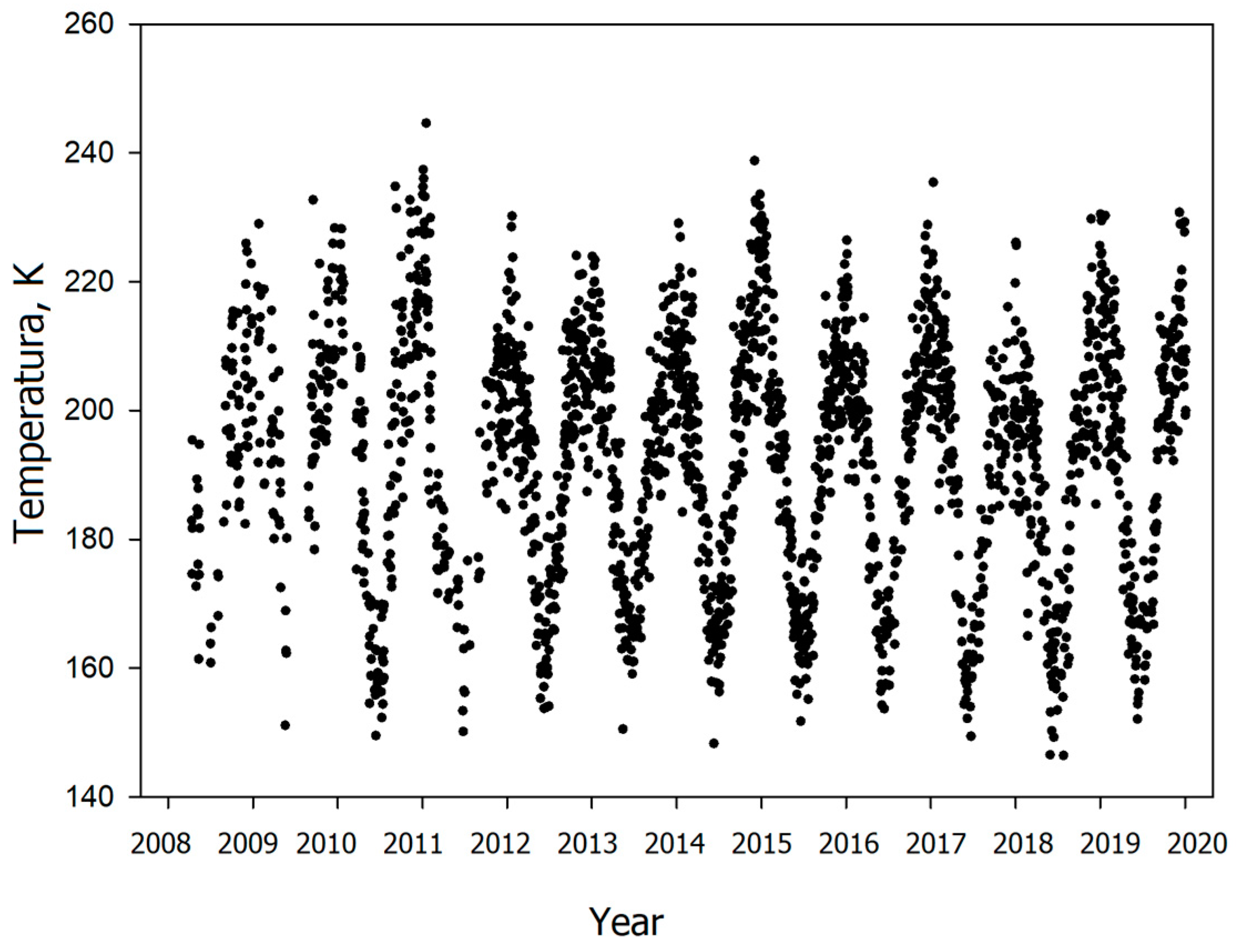
2]. This seasonal variation shows temperature differences from maximum to minimum up to 60 K throughout the year (see
Figure 1).
Other significant temperature variations are caused by different types of waves. The temperature variability occurs on timescales from days up to months in the case of planetary waves [
3,
4,
5] and on the timescale of several minutes in the case of gravity waves [
5,
6]. Day-to-day and diurnal variability of the temperature in the mesopause region is mainly caused by wave processes: planetary waves, tides, and internal gravity waves. The variability of the mesopause temperature caused by the influence of atmospheric waves of different time scales also has a pronounced seasonal dependence [
3,
4,
5,
7]. The character of seasonal changes in temperature variability can vary significantly depending on the observation region [
4,
5,
8]. Studying the long-term behavior of the upper atmosphere characteristics is very important for understanding climatic processes. Year-to-year variations and long-term trends in the mesopause temperature are of particular interest. These changes are caused by the joint influence of multi-year solar activity variations and climatic changes in the lower and middle atmosphere [
1,
9].
The year-to-year variations in the mesopause temperature there were revealed quasi-biennial oscillation, dependence on solar activity, and long-term trend see, e.g., [
1,
9,
10]. In [
9] there were reviewed the results of solar influence on mesopause temperature were obtained at various observatories from middle to high latitudes of the Northern Hemisphere. The reported sensitivities are ~1–6 K for 100 SFU (Solar Flux Unit). Recently, the 3–3.5, 4.1, and 5.5-year period oscillations characterized by observed small amplitudes have been actively studied [
11,
12]. Höppner and Bittner [
13] analyzing the mesopause temperature measurements revealed a quasi-22-year modulation of the planetary wave. Thus, in the analysis of the mesopause temperature and its variability, many factors and possible influences should be taken into account.
Year-to-year variations in the yearly average values of the ionospheric critical frequency (foF2) or peak electron density (NmF2) are very dominantly (≥95% of the total variance) controlled by solar activity represented by its proxies [
14]. The explanation for year-to-year variations in ionospheric variability is more nuanced. Forbes et al. [
15] concluded that the ionospheric variability due to day-to-day variations in solar activity is small compared to the ionospheric variability associated with geomagnetic activity. At the same time, Forbes et al. [
15] noted that this conclusion is applicable in a general statistical sense and there may be periods when 27-day solar rotation effects make a more significant contribution to ionospheric variability. Oinats et al. [
16] found that for such periods the solar activity contribution to the day-to-day variability of foF2 can reach ~70%. Rishbeth and Mendillo [
17] estimated the sensitivity of daytime NmF2 variability to geomagnetic activity as a 1% increase in variability per 1 nT increase in the Ap-index of geomagnetic activity based on the analysis of seasonal variations in NmF2 variability and Ap-index. Ratovsky et al. [
18], analyzing the year-to-year variations of the yearly average NmF2 variability, obtained a close estimation (0.8% per 1 nT) for the daytime and did not reveal a clear increase of the nighttime NmF2 variability with increasing geomagnetic/solar activity. Altadill [
19] concluded that the variability of the plasma frequency at the F-region base increases with solar activity in the post-midnight hours and does not have significant solar cycle dependence in the pre-midnight hours. Zhang and Holt [
20] revealed that the variability of electron density decreases on the bottom side of the ionosphere and increases on the top side as solar activity grows. Medvedeva and Ratovsky [
21] performed a simple linear regression analysis between NmF2 variability and indices of solar and geomagnetic activity (F10.7 and Ap). The analysis revealed a better correlation of the long-period variability with Ap than with F10.7 and the inverse relationship for short-period variability. For all period ranges, the sensitivity to geomagnetic/solar activity was higher for the daytime variability than for the nighttime one.
Comparing the variability of the parameters of the neutral atmosphere and the ionosphere, one can obtain information about the processes that determine the dynamic coupling between different regions of the atmosphere. In earlier studies, we investigated and compared the mesopause temperature and the peak electron density variabilities [
7,
21,
22]. We focused on the analysis of their seasonal variations [
7,
21], as well as a case study during the winter’s sudden stratospheric warming [
22]. We revealed both common features and distinctions in the seasonal patterns of the mesopause temperature and the peak electron density variabilities [
7,
21]. A preliminary analysis of the interannual variations of the analyzed parameters for 2008–2015 was made in [
21]. The present work continues our comprehensive study of the mesopause temperature and the peak electron density variabilities.
This paper studies year-to-year variations in the characteristics of the upper neutral atmosphere and the ionosphere over Eastern Siberia for the period of 2008–2020, covering the minima and maxima of the previous solar cycle. The mesopause temperature (Tm) obtained from the spectrometric observations of the OH(6-2) emission and the peak electron density (NmF2) from the ionosonde measurements are used as atmospheric and ionospheric characteristics. We study the annual mean Tm and yearly average values of NmF2, as well as yearly average values of day-to-day and intradiurnal variability in Tm and NmF2. To interpret the year-to-year variations, we use multiple regressions of the ionospheric and atmospheric characteristics on the F10.7-index (as a proxy of solar activity) and Ap-index (as a proxy of geomagnetic activity). For the atmospheric characteristics, we also used regressions on the SOI index.
The geographical location of the instruments providing the spectrometric and ionosonde measurements refers to the mid-latitude zone: the geographic coordinates are ~52° N and ~103–104° E, and the geomagnetic coordinates are ~42° N and ~176–177° E. Geomagnetic longitude close to 180° means that the studied region refers to the far-from-pole longitude sector. For this sector, the geomagnetic latitude is the lowest for a given geographic latitude, and the geographic latitude is the highest for a given geomagnetic latitude. Thus, the geomagnetic contribution to the variability of NmF2 and Tm is expected to be lower than in other longitude sectors for given geographic latitudes.
2. Methods
For the analysis, we used the data from spectrometric measurements of the OH ((6-2), 834 nm, ~87 km) emission carried out at the Geophysical Observatory of the Institute of Solar-Terrestrial Physics SB RAS (51.8° N, 103.1° E, Tory). The measurement methods and the data processing technique are described in detail in [
1,
23,
24]. Observations are conducted using a high-aperture diffraction spectrometer equipped with a highly sensitive digital CCD camera. The measurements are carried out at nighttime, during all nights of a year with suitable weather (cloudless, without a full Moon), the signal accumulation time is 10 min. The obtained spectra enable us to determine OH rotational temperature, which corresponds to the atmospheric temperature at the mesopause height (OH emission layer maximum is about 87 km [
1,
25].
Figure 1 shows the nightly average OH temperatures derived from the measurements. Analyzing time interval 2008–2020 includes 2185 observation nights.
To calculate both the average mesopause temperature for each year and the day-to-day and intradiurnal temperature variability, we use the method given in [
4,
5,
7,
26]. As a parameter of the mesopause temperature variability, we used the temperature standard deviations in the annual and night variations, by which one can analyze the manifestation of the various-timescale wave process activity in the upper atmosphere. Day-to-day and intradiurnal variability of the temperature in the mesopause region is mainly caused by wave processes: planetary waves, tides, and internal gravity waves. To determine the temperature’s day-to-day variability σ
dd, seasonal variations were extracted from a set of its nightly values, and then the residual temperature deviations were analyzed. The seasonal variations were calculated through the least-square fits by an annual, a semi-annual, and a terannual harmonics by the following function:
where
is the annual mean temperature,
td is the day of the year,
An and
φn are the amplitudes and phases of the harmonic
n. Fitting this formula to the temperature data gives the best possible estimate of the annual mean temperature for each year.
Figure 2 shows an example of the seasonal variation in OH rotational temperatures in year 2017 (upper panel) and differences of the measured data and the fit curve (residuals, bottom panel). After extracting of seasonal variations from the set of temperature nightly values, we analyzed temperature residuals to determine the temperature day-to-day variability σ
dd. Day-to-day temperature variations are mainly caused by planetary wave propagation in the atmosphere.
Analysis of intradiurnal temperature variations was carried out according to the method described in [
4,
5,
6]. According to this technique, the square of a given standard deviation can be represented as the sum of the squares of the standard deviations
characterizing the activity during the night of tides (σ
td2), internal gravity waves (σ
gw2), as well as fluctuations of the dark current of the spectrometer receiver (σ
n2), which are determined when the input slit of the instrument is closed. To estimate the contribution of tides in the temperature intradiurnal variations, we determined the regular night trend for each night of observations through the least square fit by the sum of the first three diurnal tide harmonics. The least-square fit for calculating the tidal contribution was used in [
5,
7,
27]. After that procedure, the trend calculated for each night was subtracted from nightly temperature sets. The values of σ
gw and σ
td were successively calculated after separating them from the series of night temperatures using the least-squares method of harmonics corresponding to the 24-, 12-, and 8-h components of the diurnal tide. This procedure was carried out for each night of observations. The calculated standard deviations σ
gw and σ
td were used as parameters characterizing temperature variability due to tides and internal gravity waves. Below, we denote σ
dd, σ
td, and σ
gw as the day-to-day, tidal, and IGW σTm.
As an ionospheric characteristic, this study uses the peak electron density NmF2, calculated from the critical frequency fof2 measured by the Irkutsk ionosonde (52.3° N, 104.3° E). Continuous ionosonde measurements allow us to consider the NmF2 as a function of local time (LT), day of the year (DoY), and year, i.e., NmF2(LT, DoY, Year). The algorithm for calculating ionospheric variability includes the following steps. The 1st step is the calculation of the 27-day running medians NmF2
med(LT, DoY, Year), which are the median values of the NmF2(LT, DoY ± 13 days, Year) series. The 2nd step is the calculation of the NmF2 disturbances (ΔNmF2), which are the percentage deviations of NmF2 from NmF2
med:
The 3rd step is the separation of ΔNmF2 into three bands of periods T using band-pass filtering: the long-period part with periods T > 24 h, the mid-period part (8 h ≤ T ≤ 24 h), and the short-period part (T < 8 h). The 4th and final step is the calculation of the NmF2 variability (σNmF2) for each period band: the σNmF2 is the root mean square of ΔNmF2 obtained by averaging over all days of each year separately for the day- and nighttime hours using ground terminator as a day-night boundary.
The long-period part of the variability (further denoted as day-to-day σNmF2) is associated with planetary waves from the lower atmosphere, day-to-day effects of geomagnetic storms, and day-to-day variations in solar activity (27-day solar rotation effects, in particular). The mid-period part of the variability (further denoted as tidal σNmF2) is associated with tidal waves from the lower atmosphere and intradiurnal effects of geomagnetic storms. The short-period part of the variability (further denoted as IGW σNmF2) is mainly associated with ionospheric disturbances generated by internal gravity waves (IGW). Rapid changes in NmF2 during geomagnetic storms can also contribute to the IGW σNmF2.
To interpret the year-to-year variations in σNmF2 in terms of solar and geomagnetic contributions, we performed multiple linear regression analyses between σNmF2 and indices of solar and geomagnetic activity. We used the yearly average F10.7-index (as a proxy of solar activity) and the yearly average Ap-index (as a proxy of geomagnetic activity). The database of these indices is available at the website
http://omniweb.gsfc.nasa.gov/form/dx1.html, accessed on 19 January 2021.
The equation of the multiple regression of σNmF2 on F10.7 and Ap has the following form:
where σ
0 is the regression intercept at F10.7 = 69 s.f.u. and Ap = 4 nT, σ
F and σ
A are the regression slopes indicating the rates of change in σNmF2 with increasing F10.7 and Ap, respectively. The intercept value (F10.7 = 69 s.f.u., Ap = 4 nT) corresponds to solar-geomagnetic conditions during the deep solar minimum of 2009. The units of σ
F (%/10 s.f.u.) and σ
A (%/nT) are chosen to give a close contribution to σNmF2 at σ
F = 1 and σ
A = 1. Considering that the range of F10.7 is 77 s.f.u., and the range of Ap is 8.3 nT in 2008–2020; σ
F = 1 gives an increase of 7.7%, and σ
A = 1 gives an increase of 8.3% from minimum to maximum.
The coefficient of determination is an important characteristic of any regression. For the multiple regression of σNmF2 on F10.7 and Ap, the coefficient of determination shows what fraction (in percent) of year-to-year variations in σNmF2 can be explained by joint variations in solar and geomagnetic activity (variations in F10.7 and Ap indices). In the case of the simple regression on F10.7 or Ap, the coefficient of determination shows what fraction of the σNmF2 variations can be explained by variations in only solar or only geomagnetic activity (only F10.7 or only Ap variations).
In the ionospheric case, we used multiple regressions of σNmF2 and yearly average NmF2 on F10.7 and Ap along with simple regressions on F10.7 and Ap. To investigate the mesopause temperature variations, we did the same for σTm and annual mean Tm and additionally analyzed regressions on the SOI index.
4. Discussion
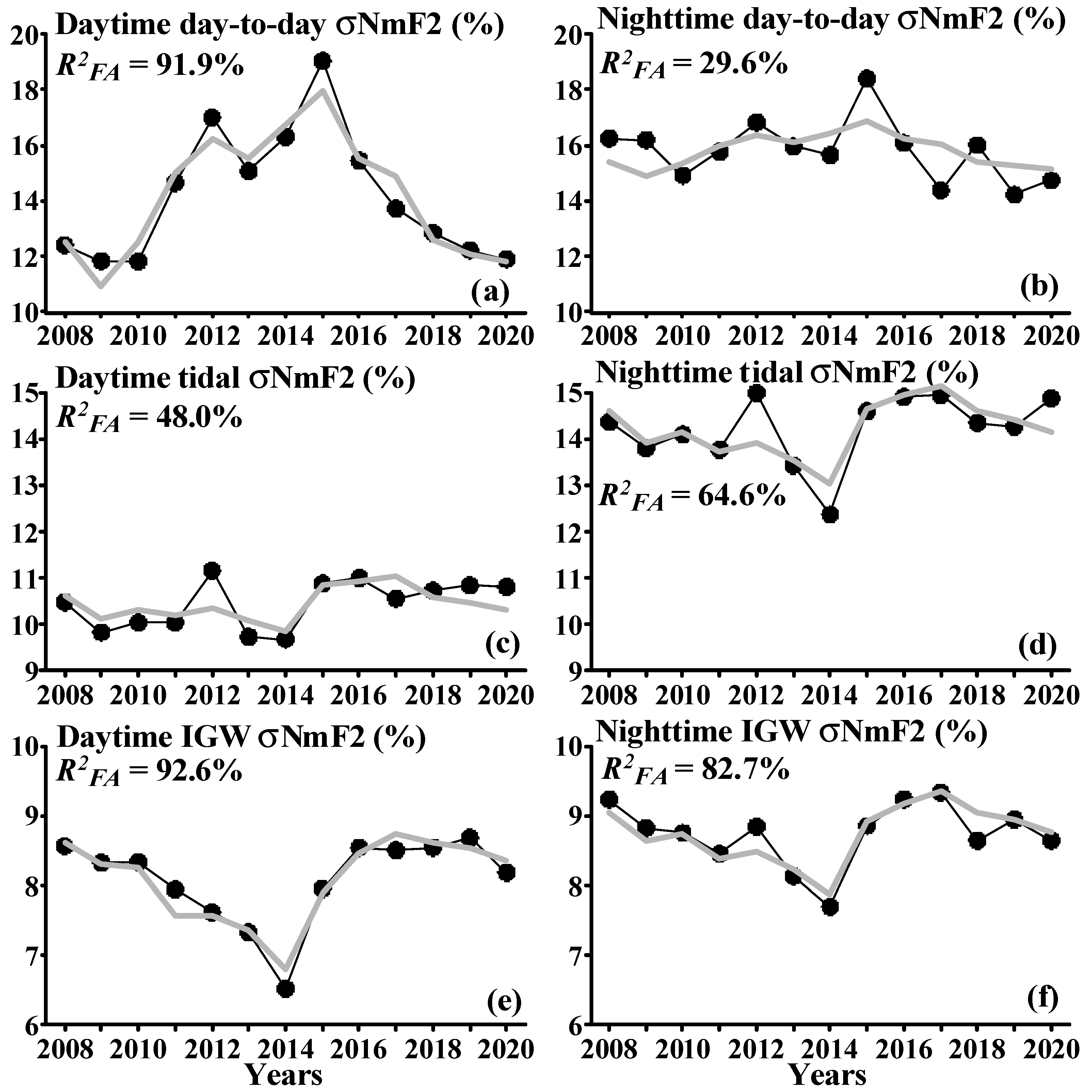
The regression analysis showed a positive correlation of the daytime day-to-day NmF2 variability with both solar and geomagnetic activity, which was initially expected, since both day-to-day variations in solar flux and the effects of geomagnetic storms increase ionospheric variability. The question is which of the factors is dominant. In
Section 3.2, we revealed that for the daytime day-to-day variability, the coefficient of determination increases from 66% for the simple regression of σNmF2 on Ap to 92% for the multiple regression of σNmF2 on F10.7 and Ap. This increase was interpreted as a comparability of the contributions from geomagnetic and solar activity to the NmF2 variability. In the year of geomagnetic maximum (2015), the geomagnetic term σ
A·(Ap-4) is 4.7% and the solar term σ
F·(F10.7-69)/10 is 2.4%, thus the geomagnetic term is ~2 times higher than the solar one. In the year of solar maximum (2014), the geomagnetic term is 2.1% and the solar term is 3.8%, thus the solar term is ~1.8 times higher than the geomagnetic one. The comparability of the contributions of geomagnetic and solar activity to the NmF2 variability is not consistent with the results of Forbes et al. [
15] and Rishbeth and Mendillo [
17] who concluded that the ionospheric variability due to day-to-day changes in solar activity is small compared to the ionospheric variability associated with geomagnetic activity. We can identify two reasons for this discrepancy. The first is that geomagnetic activity was unusually weak in the previous solar cycle 24. Rishbeth and Mendillo [
17] used Ap = 13 nT as typical (or average) geomagnetic activity, while Ap = 12.3 nT was the largest yearly average value of Ap in solar cycle 24. The largest yearly average Ap in solar cycle 24 is ~1.8 times lower than that in solar cycle 23. The second reason is the different methods for estimating the contributions of solar and geomagnetic activity. Forbes et al. [
15] used the multiple regression of the daily mean NmF2 on the annual and semiannual terms, the 81-day mean of F10.7, and the daily value of F10.7. Unlike [
15], we used the multiple regression of the NmF2 variability on F10.7 and Ap. At present, we cannot say which method is more correct, however, we can conclude the following. If the contribution of geomagnetic activity were dominant, we would not obtain a significant increase in the coefficient of determination when using the multiple regression on F10.7 and Ap compared to the simple regression on Ap.
The regression analysis showed a positive correlation between the IGW σNmF2 and geomagnetic activity, and a negative correlation between the IGW σNmF2 and solar activity. From the solar minimum in 2008–2009 to the solar maximum in 2014, the daytime IGW σNmF2 decreases by a factor of ~1.3, and the negative regression reproduces this decrease well. Given that we consider the percentage of NmF2 disturbances in accordance with Equation (1), the decrease can be associated with an increase in background NmF2 values (the yearly average NmF2 increases by a factor of ~3.1 from the solar minimum to solar maximum). If the absolute ΔNmF2 increased linearly with the background NmF2, the IGW σNmF2 would not depend on the background NmF2. If the absolute ΔNmF2 did not depend on the background NmF2, the IGW σNmF2 would decrease by a factor of ~3 from the solar minimum to the solar maximum. Apparently, a decrease in the IGW σNmF2 by ~1.3 times can be associated with the linear growth of the absolute ΔNmF2 with the background NmF2 at low background values and a saturation effect at high background NmF2. For the nighttime conditions, both the increase in the yearly average NmF2 and the decrease in σNmF2 due to solar activity are lower compared to the daytime conditions. Finally, we may assume that IGW activity does not depend on solar activity, and a decrease in σNmF2 is related to an increase in background NmF2. Both the daytime and nighttime IGW σNmF2 increase with Ap, but sensitivity to geomagnetic activity (σ
A coefficient from
Table 1) is higher for the nighttime σNmF2.
The regression analysis showed a positive correlation of the nighttime day-to-day NmF2 variability with both solar and geomagnetic activity, but sensitivity to geomagnetic/solar activity was ~3–4 times lower than for the daytime variability. Such a low sensitivity leads to a low coefficient of determination, which shows that only ~30% of the year-to-year variations in the nighttime day-to-day σNmF2 can be explained by joint variations in solar and geomagnetic activity. The absence of an increase in nighttime variability with geomagnetic activity, or even a decrease in nighttime variability with geomagnetic activity, has been noted in a number of previous studies [
18,
19,
32,
33,
34]. Among the reasons explaining this behavior, the authors identified an increase in chemical control (or recombination rate) with increasing geomagnetic activity, which reduced the amplitude of nighttime NmF2 disturbances. Another reason may be associated with nighttime NmF2 disturbances caused by geomagnetic storms related to corotating interaction regions (CIR-storms) [
35,
36]. The CIR-storms can occur under low values of the Ap index and enhance the nighttime variability in years of geomagnetic minimum. For this kind of geomagnetic activity, the Ap index may not be a proper indicator. In this case, the σ0 coefficient includes contributions from both meteorological activity and geomagnetic activity that is not identified with the Ap index.
The tidal variability of NmF2 qualitatively agrees with the IGW variability. The sensitivity to geomagnetic activity (σ
A coefficients from
Table 1) increases from the IGW to the tidal range, which indicates a greater contribution of intradiurnal effects of geomagnetic storms to the tidal range. The sensitivity to solar activity (σ
F coefficients from
Table 1) increases from the IGW to the tidal range for the nighttime and decreases for the daytime. It is not clear what could be the reason for this difference.
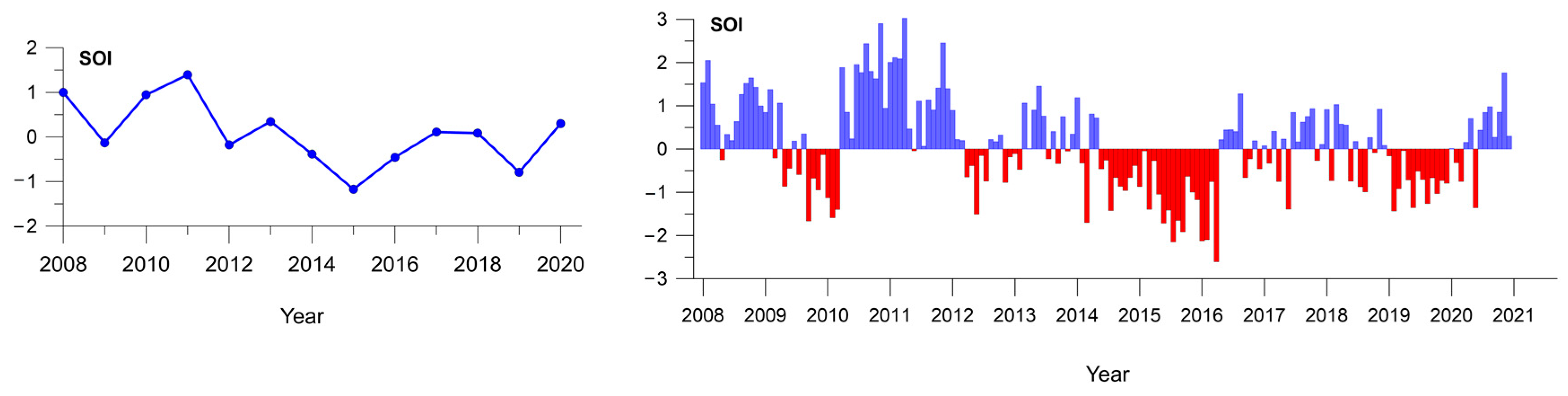
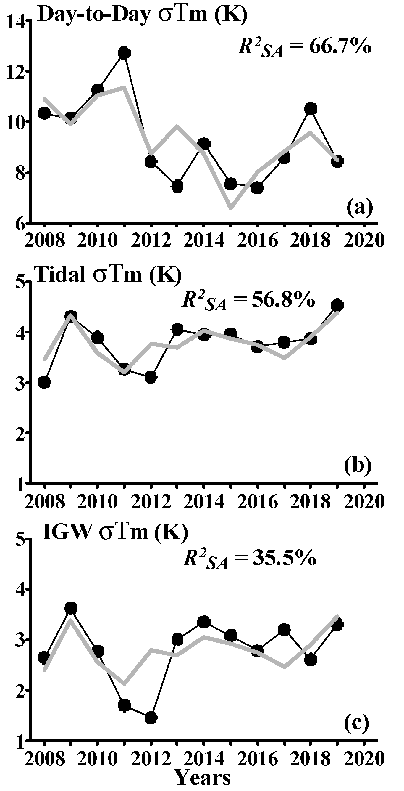
The inclusion of the SOI index in the multi-regression analysis led to a significant increase in the determination coefficients for the mesopause temperature variability. This may indicate the influence of the El Niño/ La Niña phenomena on the characteristics of the upper mid-latitude atmosphere. It was found, that the intradiurnal atmospheric variability due to the tides and IGWs (
Figure 7, middle and bottom panels) shows a negative correlation with the SOI index, with the lowest variability near the La Niña phase (2011–2012).
In [
36], based on Whole Atmosphere Community Climate Model simulations, it was revealed, that significant year-to-year variability occurs in migrating and nonmigrating tides in the mesosphere and lower thermosphere (MLT) due to the El Niño Southern Oscillation (ENSO). It was shown that the tides exhibit the largest response to the ENSO. Pedatella and Liu [
27] demonstrate, that the ENSO should be considered a potentially significant source of variability in the upper atmosphere. Thus, the observed increase in the intradiurnal variability of the mesopause temperature during the El Niño phase can be associated with an increase in the variability propagating semidiurnal tide [
28].
The analysis of day-to-day atmospheric variability caused by the migrating planetary waves (
Figure 7, upper panel) revealed a positive correlation with the SOI index, with the highest variability in the La Niña phase (SOI maximum in 2011) and the lowest variability in the El Niño phase. This contradicts the conclusion of [
28,
29] that a significant enhancement in planetary wave activity occurs during El Niño time periods. In [
26], based on model simulation, it was concluded, that at low latitudes during El Niño time periods, anomalous westward zonal mean zonal winds occur between 40 and 60 km, and anomalous eastward winds occur between 60 and 90 km. The opposite response occurs during La Niña time periods. Sassi et al. [
29] also revealed that the ENSO drives variability in the low-latitude stratosphere and mesosphere. However, in [
37] no significant variability at low latitudes was found. The possible reason for this discrepancy may be related to the use of different models in [
28,
29,
38] as well as the selection of ENSO events.
In [
4,
5,
8] it was found differences in the mesopause temperature variability for different analyzed regions. The discrepancy between our result (increase in day-to-day atmospheric variability in the La Niña phase) and the results of [
28,
29] (increase in planetary wave activity in the El Niño phase) can be explained by the latitudinal and longitudinal differences between the analyzed regions.
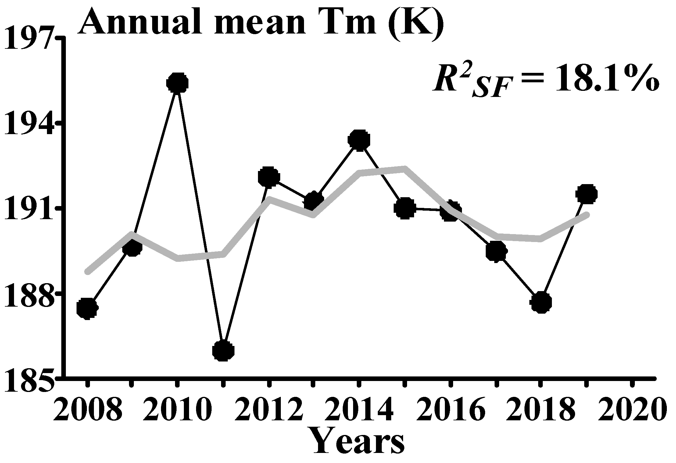
Multiple regression analysis between the annual mean mesopause temperature and SOI and F10.7 indices show low coefficients of determination. None of the indices reproduces a sharp increase of Tm in 2009–2010 and a sharp drop in 2010–2011. Sun et al. [
30] examined the influence of the El Niño–Southern Oscillation (ENSO) on the ionospheric total electron content (TEC) and concluded, that the contribution of the ENSO cold phase in 2010 and 2011 to the quasi-biennial oscillation in the TEC variations is not negligible. Probably, the variations of the annual mean temperature in 2009–2011 were influenced by the cold phase of La Niña and the highest SOI values in the last 70 years.
The multiple regression analysis between the σNmF2 and F10.7 and Ap indices revealed high coefficients of determination, except for the case of the nighttime day-to-day σNmF2. At the same time, the multiple regression analysis between the σTm and F10.7 and Ap indices revealed low coefficients of determination. The inclusion of the SOI index in the analysis of σTm led to a significant increase in the coefficients of determination. From this, we can conclude that year-to-year variations in σNmF2 and σTm are due to different reasons. The year-to-year variations in σNmF2 are mainly associated with changes in geomagnetic and solar activity (with the exception of nighttime day-to-day σNmF2), while the year-to-year variations in σTm are mainly associated with changes in activity in the underlying atmosphere. The year-to-year variations in the nighttime day-to-day σNmF2, being weakly correlated with the F10.7 and Ap indices, did not reveal a noticeable correlation with the year-to-year variations in day-to-day σTm (coefficient of determination is ~5%). It can be assumed, that changes in the activity of the underlying atmosphere make an additional contribution to the NmF2 variability with respect to changes in geomagnetic and solar activity. However, the year-to-year variations in the deviations of σNmF2 from their regressions on F10.7 and Ap did not reveal a significant correlation with the year-to-year variations in σTm (coefficients of determination < 20%). Thus, this study did not reveal a significant relationship between the year-to-year variations in σNmF2 and σTm.
5. Conclusions
The multiple regression analysis between NmF2 variability and indices of solar and geomagnetic activity (F10.7 and Ap) allowed us to obtain the following results. The multiple regression significantly increases the coefficient of determination compared to the simple regression for 4 out of 6 types of variability, which means that the contributions of geomagnetic and solar activity to the NmF2 variability are comparable for these cases. The correlation between the NmF2 variability and Ap is positive for all types of variability. The correlation between the NmF2 variability and F10.7 is positive for day-to-day variability and negative for intradiurnal variability. The positive correlation with the Ap index is explained by the contribution of NmF2 disturbances associated with geomagnetic storms and disturbed geomagnetic conditions. The positive correlation with the F10.7 index is explained by the contribution of NmF2 disturbances associated with day-to-day variations in solar flux. The negative correlation with the F10.7 index may be explained by an increase in background NmF2 due to increasing solar activity (a detailed explanation is given below).
The comparability of the contributions of geomagnetic and solar activity for the daytime day-to-day variability is not consistent with the previous studies, where it was indicated that the solar contribution is small compared to the geomagnetic one. This discrepancy can be explained by unusually weak geomagnetic activity in the previous solar cycle 24 and different methods for estimating the contributions of solar and geomagnetic activity.
The negative correlation between the intradiurnal NmF2 variability and solar activity can be explained by the following factors: (1) we consider the percentage of NmF2 disturbances relative to the background NmF2 values; (2) the background NmF2 increases with solar activity; (3) the absolute NmF2 disturbances increase linearly with the background NmF2 at low background values, and a saturation effect takes place at high background NmF2.
The lowest coefficient of determination (~30%) of the multiple regression was obtained for the nighttime day-to-day variability, which indicates that only ~30% of the year-to-year variations in the nighttime day-to-day variability can be explained by joint variations in solar and geomagnetic activity. From the analysis of previous studies, we identified two reasons for this effect. The recombination rate increases with geomagnetic activity, which reduces the amplitude of nighttime NmF2 disturbances. The nighttime NmF2 disturbances can be caused by CIR-storms that occur under low values of the Ap index, which enhances the nighttime variability in years of geomagnetic minimum.
For the first time, multiple regression analysis between the mesopause temperature, its variability, and indices of solar F10.7 and geomagnetic Ap activity, as far as Southern Oscillation Index (SOI) is performed. It was found, that involving the SOI in the analysis significantly improved the coefficients of determination for the temperature variability. Intradiurnal temperature variability shows maximum values in the El Niño phase, which is consistent with [
28]. Day-to-day temperature variations correlate with SOI variations, with maximum variability observed in the La Niña phase. Sharp variations of the annual mean mesopause temperature in 2009–2011 were probably influenced by the cold phase of La Niña and the highest SOI values in the last 70 years.
The year-to-year variations in the NmF2 variability and Tm variability are due to different reasons: in the NmF2 case, the year-to-year variations are mainly associated with changes in geomagnetic and solar activity (with the exception of nighttime day-to-day σNmF2); while in the Tm case, they are mainly associated with changes in activity in the underlying atmosphere. Thus, the study did not reveal a significant relationship between the year-to-year variations in the NmF2 variability and Tm variability.


