1. Introduction
Quantities such as irradiance and heating rates have complex spectral line structures, which vary widely from one atmospheric scenario to another. The complexity of spectral irradiance is demonstrated in
Figure 1. The values of spectrally integrated irradiances and heating rates depend on the vertical prevalence and distribution of different trace gases in the atmosphere. Water vapor plays an important role, but variations in other trace gas concentrations, as well as clouds, have a large impact on their integrated value.
Figure 2 shows simulated irradiances at the top of the atmosphere, without gas absorption, and irradiances including absorption by only one of the trace gases H
2O, CO
2, and O
3 at a time.
To model the irradiances throughout the atmosphere, one needs to represent the complex structure of the spectral absorption. A straightforward approach to calculating spectrally integrated irradiances would be to choose a fine spectral resolution with a high number of sampling nodes. This has the disadvantage that about 100,000 nodes are required for a precise calculation of the thermal spectrum, which is computationally expensive. To minimize computational time, smarter methods have to be applied.
One such method [
2] is the correlated-k approximation approach. Instead of integrating radiative quantities over wavelength nodes, this method introduces a distribution function of absorption cross-sections, which defines a corresponding probability for their occurrence. This distribution is a more tractable, continuous function, in contrast to a spectrum. To calculate the irradiance, an integral over the smoother distribution of the absorption cross-section space is performed. This approach is also recurring in a recent paper by [
3], where user-specified bands are partitioned into subbands, and the correlated-k approximation is applied. Several groups are working on such parameterizations at present, employing low amounts of wavelength bands to reduce computational cost.
The methods introduced by [
4,
5] for shortwave resp. longwave radiative transfer avoid monochromatic calculations by considering equivalent grey systems instead. The thermal spectrum is then separated into spectral bands, which are each parameterized via the Malkmus band-model.
A different approach is proposed by [
6,
7], who introduced methods using a weighted mean with representative wavelengths. These methods seek to identify wavelength sampling nodes, for which the monochromatic atmospheric quantities determine the optimal corresponding integrated quantities for different atmospheric scenarios using a weighted mean. Both approaches include a training set, on which well-performing wavelength nodes are identified and subsequently verified by a different testing set. In [
6], the targets of the method were radiances for satellite channels, while in [
7], the radiances and irradiances for spectral bands of different widths, as well as satellite channels, were targeted.
This work uses a similar approach, but instead of targets, the integrated thermal spectrum is used for optimization. The introduced method allows for the calculation of integrated irradiances and heating rates for any atmospheric scenario while reducing the computational time by several orders of magnitude compared to line-by-line calculations. An optimal set of sampling nodes, as well as corresponding weights, are determined to replace the integration over wavelengths by a weighted sum. The method involves the following steps: first, from a training set of atmospheres [
1], the corresponding altitude-dependent absorption optical thicknesses are calculated. These are obtained through the atmospheric radiative transfer simulator (ARTS) line-by-line model by [
8] using the high-resolution transmission molecular absorption database (HITRAN) 2012 line catalogue [
9] as input. We applied the lookup-table method described by [
10], which allows for us to obtain absorption cross-sections for arbitrary temperatures and pressures by interpolation from a lookup-table. Additional interpolation in teh water-vapor mixing ratio is necessary due to the self-interaction between water-vapor molecules. The next step involved the calculation of spectral irradiances using the previously calulated optical thicknesses by solving the radiative transfer equation, neglecting scattering (Schwarzschild approximation) in the thermal spectral range. This approximation can used to find representative wavelengths, since scattering properties are a comparatively smooth wavelength function. Please note that this simplified solver is only used to determine an optimized set of wavelengths, which can then be applied, together with any radiative transfer solver of arbitrary complexity. The simplification is only required to keep the computational cost of the optimization process reasonably low. For each atmosphere layer in the training dataset, upward and downward high-spectral-resolution (HSR) irradiances, as well as their integral over the full thermal spectral range, were calculated. Using the simulated annealing algorithm, as described in [
6], a set of wavelength nodes and corresponding weights were determined, so that the weighted sum of the monochromatic irradiances could optimally approximate the integrated irradiances in the training dataset.
The determined set of wavelength nodes and weights was then applied to a different testing dataset for verification. For this purpose, subsets of the 5000 atmospheres in the dataset by [
11] were employed. This dataset covers the complete spatial and seasonal variability in atmospheric profiles sampled to verify radiation models. We tested the applicability of the method for clear and cloudy atmospheres, as well as for different radiative transfer solvers.
2. Thermal Radiative Transfer Model
Since the scattering properties are smooth (compared to molecular absorption) wavelength functions, these suffice to model the radiative transfer without scattering in a plane-parallel setting for the optimization process. To simulate the irradiances and heating rates under different atmospheric scenarios, the Schwarzschild equation was solved
with the cosine of propagation zenith angle
, wavelength
, radiance
, optical thickness
and the Planck-function
.
Spectral upward and downward irradiance
on each level was recursively calculated via
where the index
i represents the level index for irradiance
and the layer index for the absorption optical thickness
. Upward irradiance at the surface, as well as downward irradiance at the top of atmosphere, are set to
where
denotes the surface temperature and
N the uppermost level of the atmospheric profile. Equation (
2) is an approximate solution of the Schwarzschild Equation (
1). To reduce computational cost, we considered only one propagation direction (
= 0.5) and used this as an approximation of the irradiance.
The heating rate
H is defined as the temperature tendency
, usually calculated from the divergence in the net flux. For the Schwarzschild model introduced above, this amounts to
where
p denotes the pressure,
the standard acceleration of gravity and
for the heat capacity of air.
Training and testing datasets contain vertical atmospheric profiles of the volume mixing ratio (VMR) of trace gases, pressures as well as temperatures. The VMR of a gas is defined as the volume fraction of the trace gas. Optical thicknesses were calculated from the pressure, temperature and given VMRs
on each layer for each trace gas in the following way
The are the absorption cross-sections of the considered trace gases, and is the number density of the air in layer i. For layer properties such as temperature, water vapor concentration and pressure, the average values on the adjacent levels were determined.
The number density
of layer
i is determined using the hydrostatic equation:
being the Avogadro constant and
the molar mass of dry air.
Absorption cross-sections vary the most strongly with respect to wavelength, due to the discrete nature of the energy transitions allowed in the molecules contained in the atmosphere. For this reason, interpolation is not performed in the wavelength and absorption cross-sections are stored on a grid with 100,000 wavelength nodes.
The shape of the absorption lines also has a significant dependency on pressure and temperature due to Doppler- and pressure-broadening. In addition to the spectral lines, the continuum needs to be considered, which is a non-linear function of the VMR in case of the self-continuum. The absorption cross-section of water vapor, therefore, is dependent on its own VMR
For the absorption line parameters, data from the HITRAN2012 molecular spectroscopic database were chosen [
9], while MT_CKD (Mlawer-Tobin-Clough-Kneizys-Davies) version 1.0 was used as water vapor continuum model [
12], which is consistent with HITRAN2012. With the atmospheric radiative transfer simulator ARTS [
13], absorption cross-sections were calculated for 100,000 wavelengths between 4 μm and 200 μm on a set of different pressure, temperature and VMR values of H
2O (called perturbations in ARTS) to encompass all atmospheric variations in the datasets of [
1,
11].
The parameters used in ARTS are specified in
Table 1. The calculation of optical thicknesses from the lookup table was implemented on the basis of the method described in [
10].
As the absorption cross-sections vary with temperature, pressure, and in case of H
2O with its own VMR, an interpolation method was developed, which optimally considers these dependencies. For a general trace gas, the method first identifies the position of the desired absorption cross-section
in the grid of the stored absorption cross-sections, producing the following four values:
Next, a bilinear interpolation of the absorption of cross-sections in terms of pressure and temperature is conducted, via a polynomial of the form
with
The polynomial parameters are determined via the four adjacent datapoints on the corners of its domain.
In the special case of water vapor, considering its dependence on its own VMR, the position of the desired absorption cross-section
in the grid of the stored absorption cross-sections produces eight values:
In this case, the interpolation via the polynomial in Equation (
10) was first conducted in
and temperature for
and
each. Both values were then linearly interpolated with respect to the pressure
.
The accuracy of the interpolation method was tested by comparison with line-by-line (LBL) calculations of optical thicknesses with ARTS in the U.S. Standard Atmosphere [
14]. Upward and downward irradiance on each level were simulated using the optical thicknesses derived from the lookup table by interpolation, and optical thicknesses calculated line-by-line using ARTS. The absolute RMSE between the two simulations was 0.87 Wm
−2. This discrepancy, however, did not affect the optimization process, since both the to be approximated values and the approximations use the same interpolation.
To include clouds in the simulations, the following simplified approach was implemented: for one layer of the atmospheric profile the absorption’s optical thickness uniformly increased by throughout the entire spectrum, a reasonable assumption since the cloud optical thickness only weakly depended on its wavelength.
4. Performance of the Parameterization
This section examines how the annealing algorithm performs for different parameters and discusses the characteristics of the chosen sampling nodes. The amount of sampling nodes, as well as the amount of annealing iterations, contribute to a more accurate result.
In
Figure 3, the performance of a reduced lookup table with 10 and 100 wavelength sampling nodes is displayed for different numbers of annealing iterations. For each datapoint, the average and standard deviation of thirty simulated annealing runs on a set of 6000 irradiance values are shown. It becomes clear that, for a given number of sampling nodes, the minimum error converges to a lower bound, which cannot be improved by the addition of more annealing iterations. The limit reached at the right end of the plot indicates the maximum possible accuracy for a given number of sampling nodes.
As noted in [
6], the values for annealing start temperature and end temperature, as well as the amount of annealing iterations, had to be chosen to avoid wasting computational time or depriving the algorithm of the chance to try new, potentially better wavelengths.
In
Figure 3, the annealing result is shown to continually improve with the number of annealing iterations. It can be observed that there is significant potential for improving the result, particularly for low iteration numbers. This progress is, however, slowing down so that further calculations would not improve the result and waste calculation time. For the purpose of these calculations, a total iteration number of
10,000 was determined to be sufficient.
In
Figure 4, the wavelengths and corresponding weights for four different annealing runs with different numbers of sampling nodes are displayed. Some information about the position and weights are summarized in
Table 3. At least three conclusions can be drawn:
The linear regression method produces few negative weights. These did not produce any unphysical results during testing.
Sampling nodes concentrate on the part of the spectrum in which most of the absorption of different trace gases takes place. This can be seen by comparing to the impact of trace gas absorption (CO
2, H
2O and O
3) in
Figure 2.
Comparatively large weights at longer wavelengths, where little absorption takes place, account for the bulk of the integrated value, while sampling nodes at shorter wavelengths with high absorption determine the fine-tuned values with respect to specific atmospheric scenarios.
Figure 4.
Positions of sampling nodes and chosen weights from reduced lookup tables for 10 (a), 30 (b), 50 (c) and 100 (d) sampling nodes.
Figure 4.
Positions of sampling nodes and chosen weights from reduced lookup tables for 10 (a), 30 (b), 50 (c) and 100 (d) sampling nodes.
Table 3.
Fraction of sampling nodes in weight and wavelength ranges.
Table 3.
Fraction of sampling nodes in weight and wavelength ranges.
| | | | | |
|---|
| 10 | 0.70 | 1.00 | 0.20 | 0.70 | 0.00 |
| 30 | 0.73 | 0.87 | 0.63 | 0.90 | 0.00 |
| 50 | 0.80 | 0.90 | 0.70 | 0.88 | 0.04 |
| 100 | 0.82 | 0.92 | 0.77 | 0.94 | 0.06 |
4.1. Test Dataset
To test the method, we used a database of [
11] containing 5000 profiles with 91 levels. These profiles were sampled from an even larger database containing 121,462,560 profiles from cycle 30R2 of the the European Centre for Medium-Range Weather Forecasts (ECMWF) forecasting system. The dataset provides an exhausting variation in atmospheric temperature and specific humidity. The database scenarios include clear and cloudy cases.
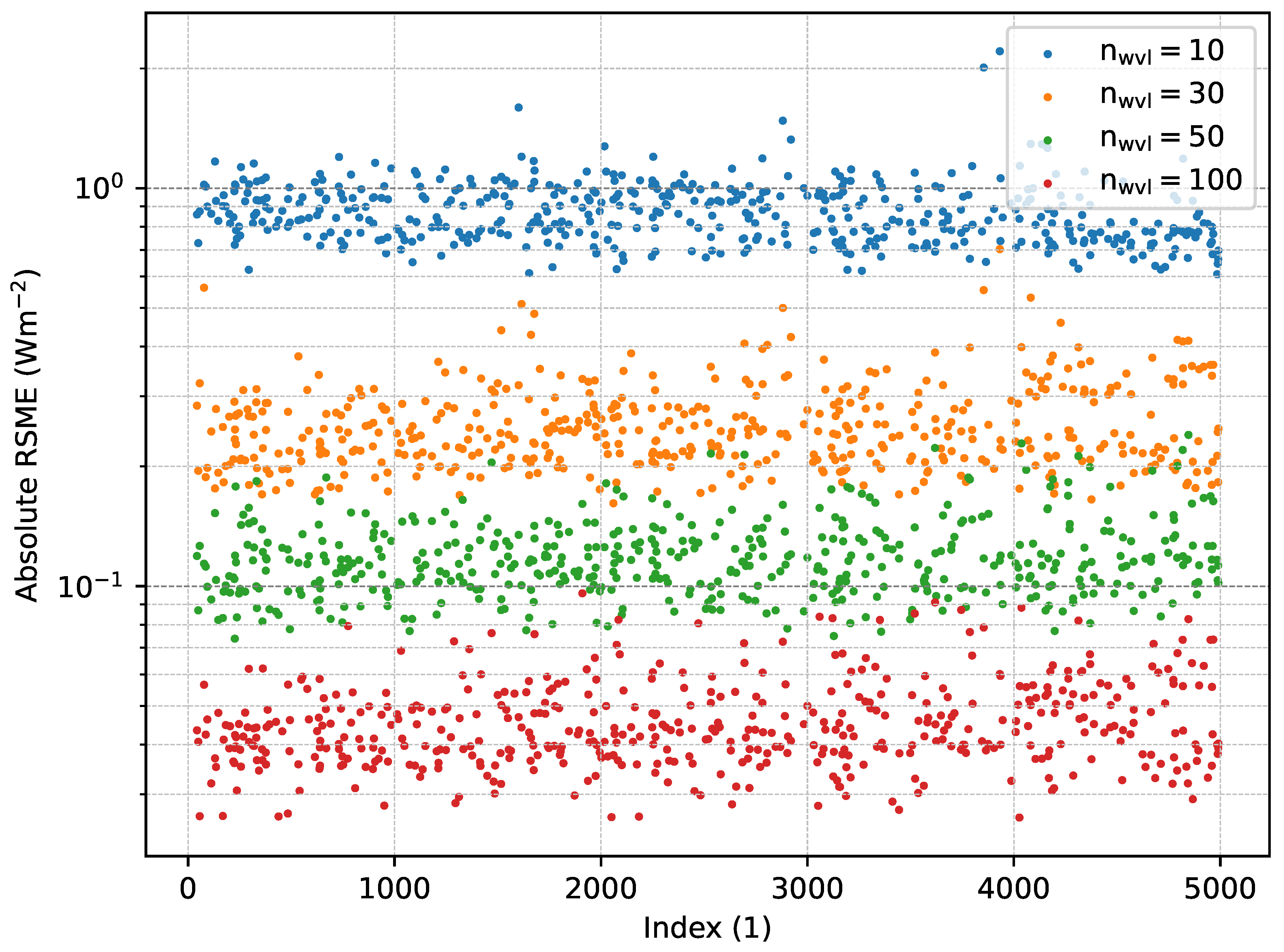
4.2. Accuracy of Irradiances
Figure 5 shows the absolute RSME of irradiances calculated by a weighted sum over representative wavelengths with respect to the accurate irradiances calculated by integration in the high-resolution spectrum. The blue dots correspond to lookup-tables including 10 representative wavelengths, the orange dots to 30 representative wavelengths, the green dots to 50, and the red dots to 100 representative wavelengths. For each reduced lookup table, the same randomly selected set of 500 atmospheres from the test dataset was used. As the figure shows, the training set of atmospheres by [
1] is sufficient for the creation of reduced lookup tables, which perform equally well for all different atmospheric scenarios from [
11].
The average errors and standard deviations of the 500 profiles in
Figure 5 are shown in
Table 4. As expected, a higher amount of sampling nodes improves the accuracy; however, the computational time linearly depends on the number of sampling nodes.
4.3. Accuracy of Heating Rates
In
Table 5, the absolute RSME of heating rates, as determined via high spectral resolution simulations and weighted sum for the U.S. Standard Atmosphere, are shown for
10, 30, 50 and 100. Low irradiance errors still result in low errors in the corresponding heating rates. Increasing the number of sampling nodes improves the accuracy of the heating rate calculations. In
Figure 6, the heating rates for the U.S. Standard Atmosphere, calculated with 10, 30 and 50 sampling nodes and HSR-simulations, are depicted. The figure illustrates the improvement in accuracy with an increased number of sampling nodes.
4.4. Cloudy Atmospheres
An important question posed in [
6] is whether this method can be applied to atmospheric scenarios involving clouds.
We modeled such a cloud by uniformly adding a value of
to the spectral optical thickness at its intended height in the atmosphere. In
Figure 7, the heating rates calculated with 10, 30 and 50 sampling nodes and HSR-simulations are depicted to add such a cloud at the 10th layer in U.S. Standard Atmosphere. This corresponds to a cloud between 500 hPa and 550 hPa.
We included this cloud layer in the 500 atmospheric profiles, whose irradiances were determined in
Section 4.2. In
Table 4, the resulting RSMEs for the same 500 atmospheres from [
11] are shown to have an extra cloud. For each of those, a cloud was added to the 22nd layer (3.1 to 3.4 km) by again adding
to the spectral optical thickness.
Comparing these errors with the errors in the original atmospheres without a cloud in
Table 4, the reduced lookup tables performed similarly, and slightly better for 10 sampling nodes. Since the errors were stable under the addition of a cloud, the validity of the reduced lookup tables for cloudy atmospheres is confirmed.
5. Conclusions
In this work, we used the simulated annealing algorithm to determine a small set of representative wavelengths to calculate integrated thermal irradiances and heating rates. Using a weighted sum approach, the computational cost of integral calculation could be decreased by several orders of magnitude. A cost-efficient lookup table approach was adopted to calculate the optical absorption thicknesses. Using a simple Schwarzschild radiative transfer model, we calculated irradiances at a high spectral resolution for various atmospheric scenarions, which could be used as training data for the simulated annealing algorithm. As the next step, for different numbers of sampling nodes, optimized lookup tables were produced, including representative wavelengths and corresponding weights. The integrated irradiance can be calculated from this table using a weighted sum of irradiances, which were calculated at the representative wavelengths. Through their application on a large test dataset, we found that ten representative wavelengths are sufficient to achieve an average RSME for irradiances below 1 Wm−2. With 100 wavelength nodes, an average RSME below 0.05 Wm−2 can be achieved. The method was verified for a large variety of atmospheric profiles taken from the ECMWF model. This performed equally well for atmospheres with or without clouds.
Throughout this work, one specific training dataset was used, which used typical atmospheric profiles from a numerical weather prediction (NWP) model. Alternatively, for radiative transfer in climate models, the training data could be extended by including higher variability in greenhouse gases to derive more precise lookup tables for these scenarios. This method could also be used to train specifically for heating rates, in order to achieve a higher accuracy in that area. The REPINT parameterization is available in the libRadtran radiative transfer package [
15,
16]. This can be used in combination with various radiative transfer solvers based on different methodologies, such as twostream or discrete ordinate, which consider scattering in 1D and 3D geometry.
In the future, we plan to extend the methodology to the solar spectral region. Here, scattering can no longer be neglected; therefore, another radiative transfer solver needs to be applied. The simulated annealing approach is expected to work equally well in the solar region, since it has already been used to generate the REPTRAN parameterization [
7] for spectral bands in both solar and thermal spectral regions.


