Article

Short-Term Prediction of 80–88 km Wind Speed in Near Space Based on VMD–PSO–LSTM

1
School of Electronic Engineering, Ocean University of China, Qingdao 266100, China
2
National Key Laboratory of Electromagnetic Environment, China Research Institute of Radiowave Propagation, Qingdao 266107, China
3
Kunming Electro-Magnetic Environment Observation and Research Station, Qujing 655500, China
*
Author to whom correspondence should be addressed.
Atmosphere 2023, 14(2), 315; https://doi.org/10.3390/atmos14020315
Submission received: 9 January 2023 / Revised: 27 January 2023 / Accepted: 31 January 2023 / Published: 4 February 2023
(This article belongs to the Special Issue Structure and Dynamics of Mesosphere and Lower Thermosphere)

Abstract

:
The accurate prediction of atmospheric wind speed in near space is of importance for both middle and upper atmospheric scientific research and engineering applications. In order to improve the accuracy of short-term wind speed predictions in near space, this paper proposes a multi-step hybrid prediction method based on the combination of variational modal decomposition (VMD), particle swarm optimization (PSO) and long short-term memory neural networks (LSTM). This paper uses the measurement of wind speed in the height range of 80–88 km at the Kunming site (25.6° N, 103.8° E) for wind speed prediction experiments. The results show that the root mean square error ( R M S E ) and the mean absolute percentage error ( M A P E ) of multi–step wind predictions are less than 6 m/s and 15%, respectively. Furthermore, the proposed VMD–PSO–LSTM method is compared with the traditional seasonal difference autoregressive sliding average model (SARIMA) to investigate its performance. Our analysis shows that the percentage improvement of prediction performance compared to the traditional time series prediction model can reach at most 85.21% and 83.75% in R M S E and M A P E , respectively, which means that the VMD–PSO–LSTM model has better accuracy in the multi-step prediction of the wind speed.

1. Introduction

Near space covers the altitude region of approximately 20–100 km, which is the transition region between the lower atmosphere and the upper atmosphere with very complex dynamic processes [1]. It is the resident area for various high-altitude balloons, high altitude vehicles, suborbital vehicles and low orbiting spacecraft [2]. The atmospheric parameters have an important impact on the design and safe operation of the various vehicles. For example, the temperature in near space directly affects instrument performance and material temperature fatigue damage of the vehicle, ozone is very corrosive, density and wind fields affect the attitude and position of the near-space vehicles and neutron radiation can cause single-particle effects, etc. [3]. As one of the most critical parameters in the atmospheric dynamics of near space, the atmospheric wind field directly affects reliable operation of the near-space vehicles. For example, the residency ability of vehicles depends on the wind field environment [4], and high-altitude solar UAVs’ pneumatic characteristics and range are also importantly affected by the wind [5]. Therefore, it is important to conduct research on the wind field in near space and obtain accurate wind field prediction information for the mission planning, trajectory planning and flight control of near space vehicles [6].
At present, wind speed prediction methods in near space mainly include two types: the numerical weather prediction method and the statistical model method [7]. Numerical weather forecasting requires complex physical models and large computational systems to obtain predicted values of wind speed, wind direction, temperature, humidity and other meteorological elements through meteorological theory and computational fluid dynamics [5]. The statistical modeling method mainly adopts the idea of mathematical statistics to make predictions by mining the inherent laws existing among data [5]. Statistical models are mainly divided into continuous models, classical statistical models and artificial intelligence models. Among them, classical statistical models are mainly time series forecasting models, such as the autoregressive moving average (ARMA), seasonal autoregressive integrated moving average (SARIMA), etc. The artificial intelligence models are mainly neural network models, such as recurrent neural networks (RNN), long short-term memory (LSTM), etc. Conventional numerical weather prediction systems focus on meteorological information within the troposphere that is closely related to human socio-economic activities [8]. It has been studied earlier and has advanced numerical forecasting techniques. Compared with weather forecasting, space weather forecasting is currently dominated by statistical models, and numerical forecasting techniques are in the development stage. The forecasting of the near-space atmospheric environment has just started, and statistical modeling methods still play an important role [8]. Therefore, the statistical model approach is usually used in the prediction of the wind field in near space.
The forecast height range of the near-space atmospheric environment is between meteorological forecast and space weather forecast. There are relatively few studies on the prediction of near-space atmospheric environment parameters [8]. In terms of numerical forecasting techniques, the U.S. Navy has used the global numerical prediction model of NOGAPS-Advanced Level Physics and High Altitude (NOGAPS-ALPHA) to achieve the medium-range forecasts (1–2 weeks) from the ground to an altitude of 85 km and multi-year climate forecasts [9]. In order to ensure the safe operation of high altitude vehicles, Jason A. Roney et al. studied the 18–30 km wind field in near space and built a statistical forecasting model based on the observation data in Akon, OH, USA and White Sands, NM, USA [10]. The National Space Science Center of the Chinese Academy of Sciences has developed the exploration of numerical near space forecasting, and established a global three-dimensional near space assimilation forecasting principle system [11]. In terms of statistical forecasting, Hu Xiong et al. used an autoregressive model to carry out wind speed prediction experiments at 20–100 km for the next 48 h for the Langfang area in 2014, and the results showed that the model could effectively predict the atmospheric environment in near space. However, due to the influence of small-scale atmospheric fluctuations, the predicted results had a large deviation from the actual wind field changes [12]. In 2018, Liu Tao et al. exploited the ARMA to predict zonal wind at 88 km in Langfang. The results showed that when the wind field changes regularly, the ARMA model predicts the future wind field better, but when the wind field changes significantly, the prediction of the ARMA model becomes less effective. The sudden change of wind field makes the wind speed series seriously non-stationary and stochastic, and it is difficult for the traditional time series method to solve the problem of the complex non-linear relationship of the series [8].
With the continuous development of deep learning technology, some deep learning models are gradually applied to the study of time-series data [13]. Among many deep learning models, recurrent neural networks (RNN) show better performance in time series prediction. Long short-term memory (LSTM) is an improved RNN with better long-term prediction capability and fault tolerance, which can solve the problem that RNN cannot achieve: the memory and forgetting of long-term historical information [14]. However, when the non-smooth characteristic of the sequence is strong, the local variation of wind speed cannot be accurately learned, which will make the training of deep learning methods more difficult and reduce the accuracy of model prediction [15]. Therefore, for the significantly varying wind speed series, it is necessary to decompose the wind speed series into a simple and smooth subseries by the signal decomposition method before inputting it into the neural network to simplify the network model complexity and improve the prediction accuracy [16]. The main typical signal decomposition methods include wavelet decomposition and empirical mode decomposition (EMD). However, wavelet analysis is a non-adaptive decomposition method, which relies on the selection of wavelet basis functions, and EMD is prone to the problems of modal confusion and endpoint effects, which can affect the decomposition results [17]. In 2014, Dragomiretskiy et al. proposed the variational mode decomposition (VMD) method, which can not only overcome the shortcomings of wavelet analysis and EMD, but also effectively solve the problems such as strong non-smoothness of a wind speed series [
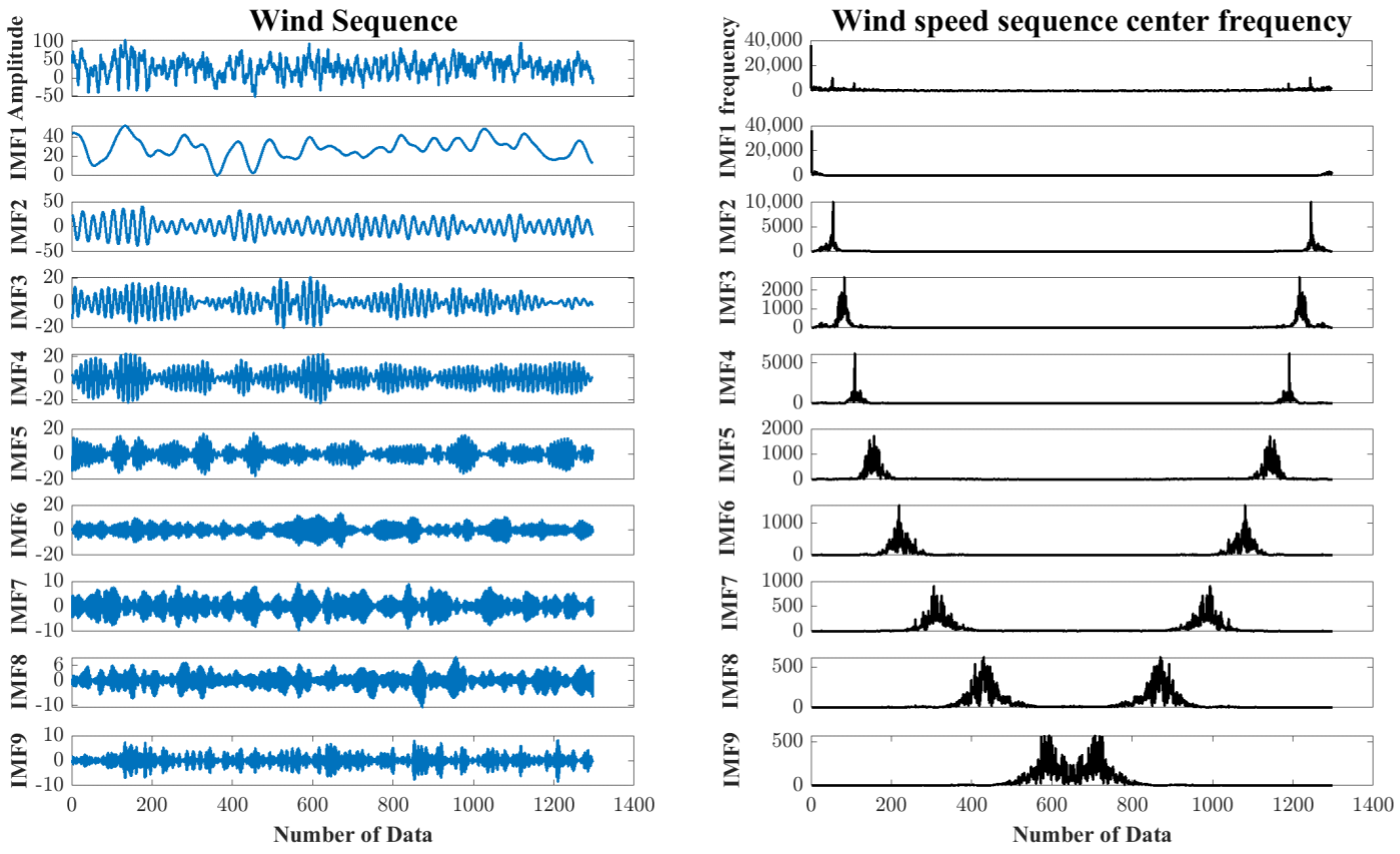
18]. VMD can decompose a wind series into multiple subsequences of different frequency scales and relative smoothness, i.e., intrinsic mode function (IMF) components [19]. Therefore, the LSTM network can be used to predict wind IMF components, and then reconstruct the corresponding prediction results, improving the prediction accuracy of the LSTM network [20]. Currently, many optimization algorithms have been used as a deep learning method to find an optimal set of parameter combinations in a short time to improve the network prediction performance [
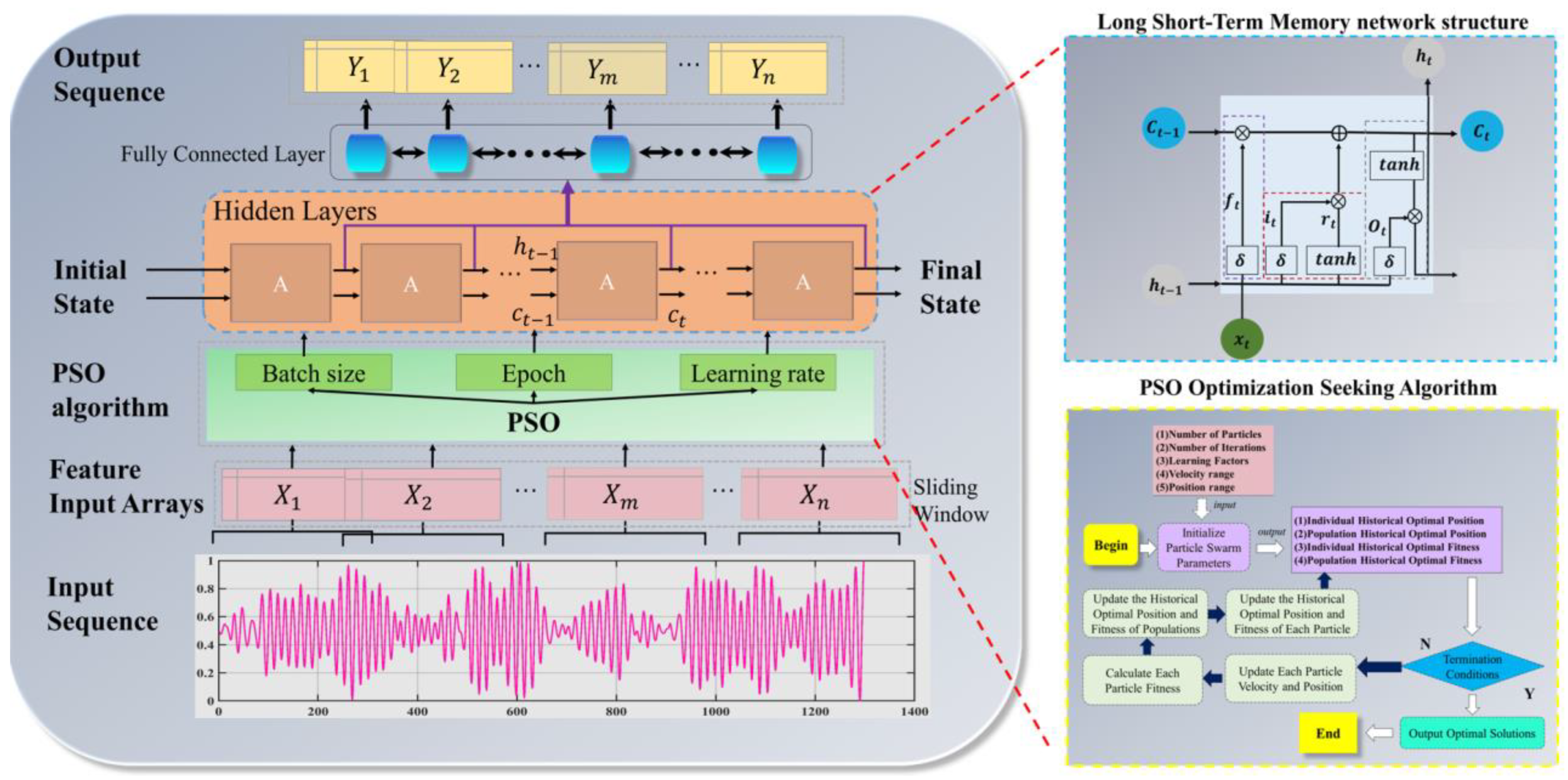
20]. The particle swarm optimization (PSO) algorithm is an efficient optimization algorithm that can find a set of global optimal solutions by constant particle updates and iterations, which has the advantages of fast convergence and high accuracy [21]. PSO can effectively optimize the hyperparameters of the LSTM network such as the batch size, epoch and learning rate to improve the prediction performance of LSTM networks [20].
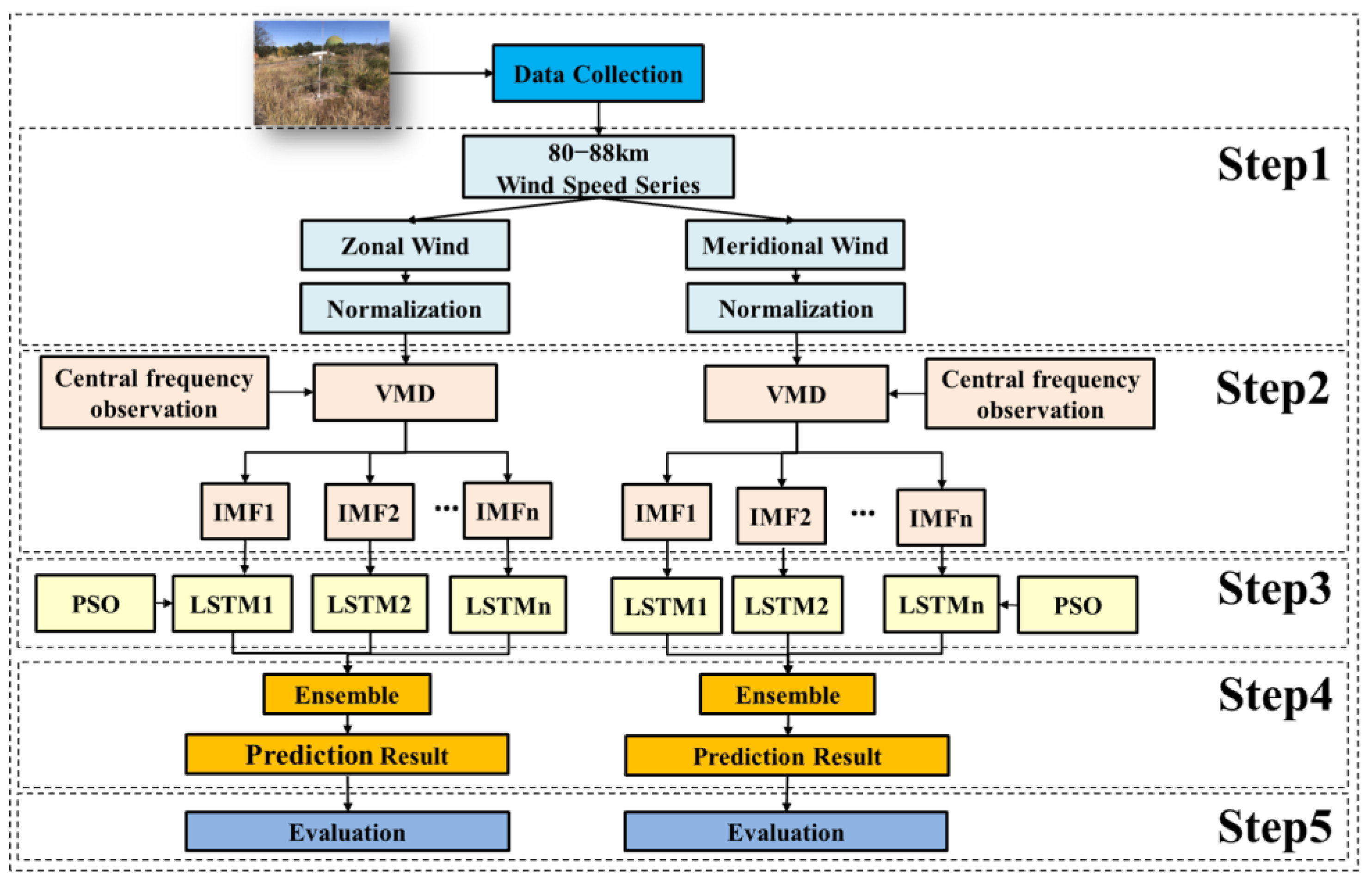
Based on the above study methods, this study proposes a novel hybrid prediction method (VMD−PSO−LSTM) by combining the VMD method, PSO algorithm and LSTM network to achieve the accurate prediction of wind speed in the upper layer of near space (80–100 km). The VMD−PSO−LSTM method is constructed as follows: (1) using the VMD method, the wind speed sequence is decomposed to obtain a limited number of smooth subsequences with different frequency scales; (2) for the decomposed subsequences (IMF components) of different scales, corresponding LSTM prediction models are built, respectively, using the PSO algorithm to optimize the hyperparameters of each LSTM prediction model, and using the optimized LSTM network to predict the subsequences; (3) the prediction results for each wind speed subsequences are reconstructed to obtain the final wind speed prediction results.
The main contents of this paper are organized as follows. Section 2 describe the general idea of constructing a hybrid model. 
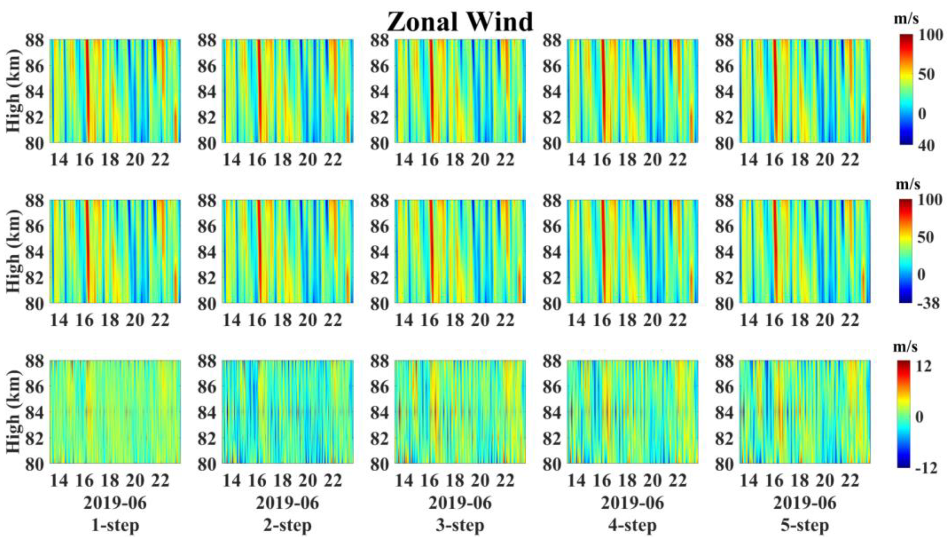
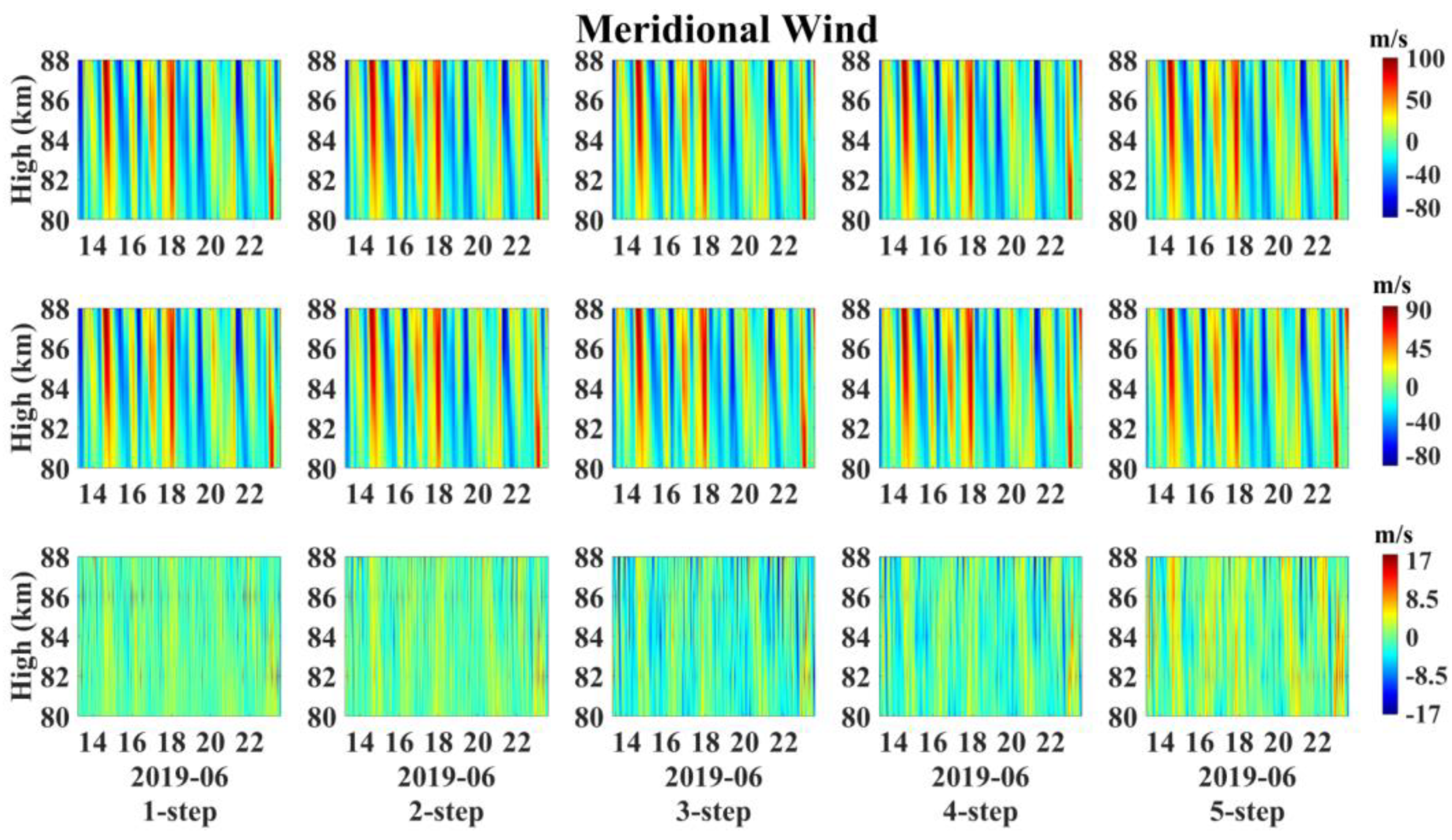
Section 3 uses a new model to conduct multi-step prediction experiments at different heights in the Kunming area. 
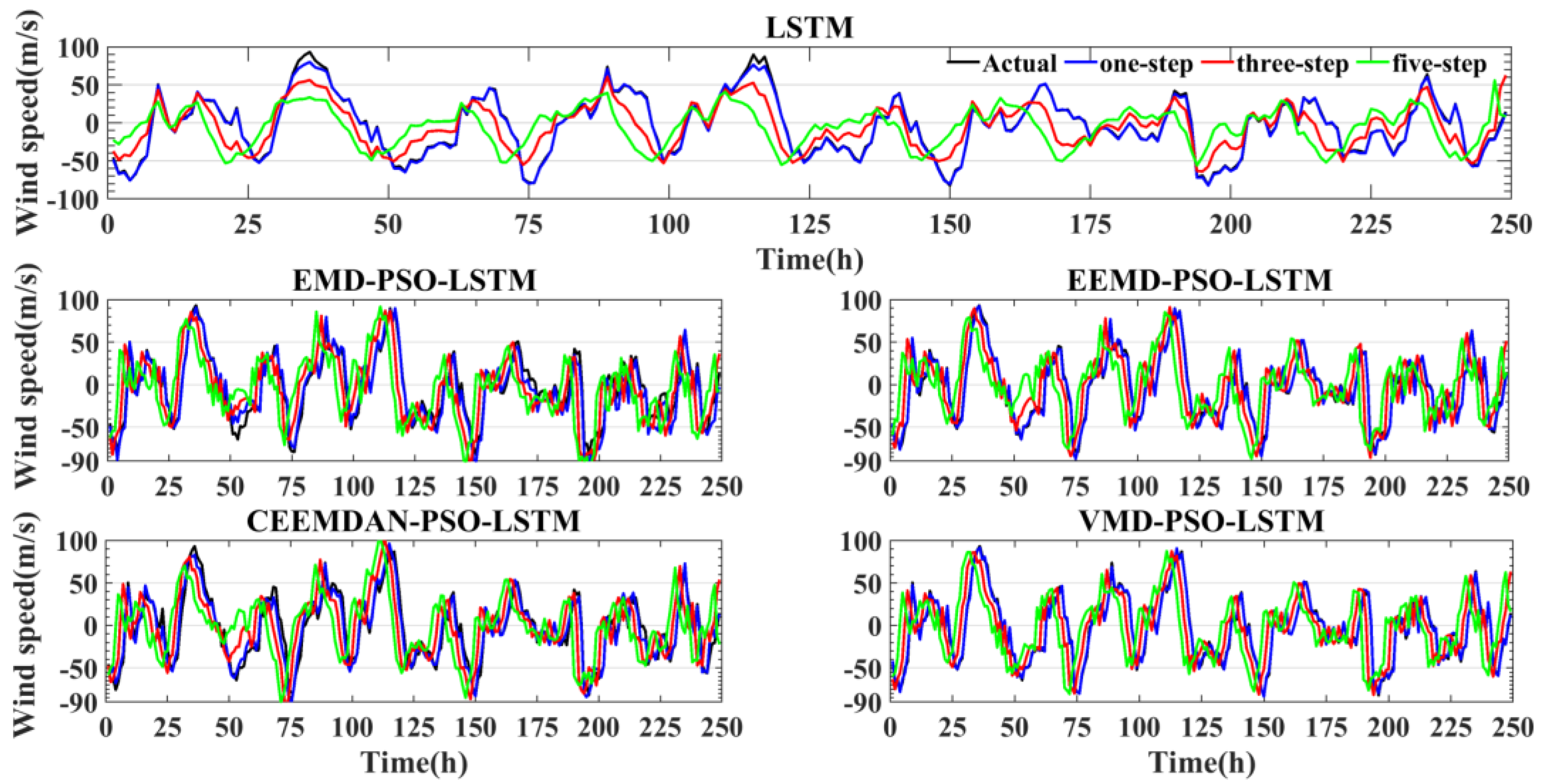
Section 4 verifies the effectiveness of the new model by building a comparison experiment between the traditional time series predictive model and the new prediction model. Section 5 summarizes the results of the study and draws experimental conclusions.

2. Network Construction

The VMD–PSO–LSTM wind speed prediction model includes five main steps: data preprocessing, variational mode decomposition, construction of the PSO–LSTM network model, IMF prediction reconstruction and model evaluation. The flow chart of model construction is shown in Figure 1.

2.1. Data Preprocessing

The measured wind field data of the Kunming meteor radar at 86 km height from 1 May to 23 June 2019 are used as the experimental data samples with a sampling step of 1 h, and the data preprocessing process is shown in Figure 2. First, the interpolation method is used to fill the invalid points. Second, to eliminate the large prediction error caused by the inconsistency of the sample data dimension, the deviation standardization method is adopted to normalize the data preprocessing. This method makes the data values between [0, 1] for each sample, and the normalization is calculated as follows:
Y = X X min X max X min
where X max and X min represent the maximum and minimum values in the wind speed subsequence, respectively.
The workload of network computation and maintenance costs are relatively large when the number of prediction time steps is high. This study uses a multioutput prediction strategy in Equation (2), where l denotes the length of the training data and Δ denotes the number of prediction steps at the overrun moment. To build the input-output data set, the continuous IMF wind speed series are transformed into n , m vector data, where n is the number of samples and m is the number of sample dimensions. m is denoted as m = l + Δ , i.e., the wind speed in the first l hours predicts the wind speed in the next Δ hours [22]. In this paper, the first 48 h are used to predict the wind speed values for the next 5 h, and the data set is divided in the ratio of 7:1:2. That is, 70% is used as the training data set for training data, 10% is used as the validation data set for network parameter optimization and 20% is used as the test set to check the network prediction performance.
p r e ( t + 1 ) , p r e ( t + 2 ) , p r e ( t + 3 ) , , p r e ( t + Δ ) = m o d e l ( r e a l ( t 1 ) , r e a l ( t 2 ) , r e a l ( t 3 ) , , r e a l ( t l ) )

2.2. Variational Model Decomposition

VMD is an adaptive and completely non-recursive approach to modal variation and signal processing [23]. VMD can decompose the wind sequence into multiple subsequences called IMF components, according to the characteristics of the wind sequence. VMD can adaptively match the optimal center frequency and bandwidth of each IMF. The main decomposition process is as follows.
(1)
In the VMD method, each IMF component is defined as a non-smooth Amplitude Modulation–Frequency Modulation (AM–FM) signal [24]:
u k ( t ) = A k ( t ) cos ( ϕ k ( t ) )
where A k ( t ) represents instantaneous amplitude and ϕ k ( t ) represents phase function.
(2)
Conducting the Hibbert transform on each IMF component u k ( t ) to obtain the unilateral frequency spectrum and analytical signal of the IMF component:
[ δ ( t ) + j π t ] u k ( t )
where “ ” represents the convolution operation, δ ( t ) represents dirac distribution, j represents the imaginary part and t represents time.
(3)
Using the exponential operator e j ω k t to modulate its spectrum to the fundamental band:
[ ( δ ( t ) + j π t ) u k ( t ) ] e j ω k t
where ω k represents the central frequency of u k ( t ) .
(4)
The bandwidth of each IMF component can be obtained from the Gaussian smoothing of the demodulated signal. With the bandwidth estimation, the constrained variational problem can be expressed as:
min { u k } , { w k } { k = 1 K t [ ( δ ( t ) + j π t ) u k ( t ) ] e j ω k t 2 2 } s . t . k = 1 K u k ( t ) = f ( t )
where u k = { u 1 , u 2 , , u k }  represents the K IMF components obtained from the decomposition of wind speed sequence f ( t ) , ω k = { ω 1 , ω 2 , , ω k }  represents the central frequency of each IMF component, and t represents the time derivative.
(5)
The constrained variational problem can be converted to an unconstrained variational problem by introducing a penalty factor α and Lagrange operator λ ( t ) . The extended Lagrange expression is:
L ( u k , ω k , λ ) = α k = 1 K t [ ( δ ( t ) + j π t ) u k ( t ) ] e j ω k t 2 2 + f ( t ) k = 1 K u k ( t ) 2 2 + λ ( t ) , f ( t ) k = 1 K u k ( t )
(6)
The above problem can be solved by the alternating direction multiplier method, and the updated u k and ω k are, respectively:
u k n + 1 ( ω ) = f ( ω ) i k u i n ( ω ) + λ n ( ω ) 2 1 + 2 α ( ω ω k n ) 2
ω k n + 1 = 0 ω u k n + 1 ( ω ) 2 d ω 0 u k n + 1 ( ω ) 2 d ω
λ n + 1 ( ω ) = λ n ( ω ) + τ ( f ( ω ) k = 1 K u k n + 1 ( ω ) )
where τ is the noise tolerance of the signal, n represents the number of iterations, and u k n + 1 ( ω ) , f ( ω ) , λ n ( ω ) represent the Fourier transform of u k n + 1 ( t ) , f ( t ) , λ n ( t ) , respectively. Iterating until the convergence condition is met or the maximum number of iterations is reached:
k = 1 K u k n + 1 u k n 2 2 u k n 2 2 < γ

2.3. Building the PSO-LSTM Network Model

(1) LSTM network structure
LSTM replaces the implicit nodes of the RNN with memory units. The purpose is to solve the problem that RNNs cannot effectively transfer historical information due to the long interval of implicit nodes [25,26]. One of the LSTM network memory cells mainly consists of memory cells and three gate controllers (forgetting gate, input gate and output gate) [27], as shown in Figure 3. The three gates are all a function of the input feature x t at the current moment and the short-term memory h t 1 at the previous moment. The detailed processes are as follows.
The first step of the LSTM network is to select the forgetting of information in the cell state. This step is determined by the forget gate. The output h t 1 and input x t are input into the sigmoid activation function and the output is a number between 0 and 1 to each number in the cell state c t 1 at the previous moment, 1 represents the “fully keep” state and 0 represents the “fully forget” state. The calculation equation of the forget gate is as follows:
f t = σ ( W f [ h t 1 , x t ] + b f ) ,
The next step will determine what wind speed characteristics information will be saved in the current cell state. This step is determined by the input gate. This step consists of two parts. One is the input state i t whose values need to be updated by the sigmoid function σ , and the other is the candidate state c ˜ t which adds to the memory unit state by the tan activation function. The input gate is calculated as follows:
i t = σ ( W i [ h t 1 , x t ] + b i ) ,
c ˜ t = tanh ( W c [ h t 1 , x t ] + b c ) ,
Then this step is to update the old cell state c t 1 to the new cell state c t . c t is equal to the sum of the value of the long-term memory c t 1 at the previous moment through the forgetting gate and the value of the new knowledge c ˜ t generalized at the current moment through the input gate. The new state c t is calculated as follows:
c t = f t c t 1 + i t c ˜ t ,
Finally, the next step will determine what information will be output. This step is determined by the output gate and the newly obtained cell state c t . The output h t 1 and input x t are input into the sigmoid activation function, and c t is then input into the tanh activation function; subsequently, the two parts are multiplied as follows:
o t = σ ( W o [ h t 1 , x t ] + b o ) ,
h t = o t tanh ( c t )
where f t represents the forget gate, x t represents the input gate and o t represents the output gate; c t represents the cellular state of long-term memory, and c ˜ t represents the candidate state waiting to be stored in long-term memory; h t 1 represents the short-term memory of the previous moment, and h t represents short-term memory of the current moment; W f , W i , W c , W o represent the weight vector matrix corresponding to the three gates; b f , b i , b c , b o represent biasing terms. σ and tanh represent the sigmoid activation function and hyperbolic tangent activation function, respectively, and are calculated as follows [20]:
sigmoid = 1 1 + e X
tanh = e X e X e X + e X
(2) PSO Optimization Search Process
From Figure 3 and Equations (12)–(17), the LSTM network implicitly contains a variety of internal parameters, and some of them need to be set artificially [28]. However, the prediction performance of the models trained with different parameters varies widely. Therefore, this paper introduces the PSO algorithm of the adaptive learning strategy to find the key parameters of the LSTM model [29,30]. The specific process is shown in Figure 3. The main optimization process is as follows.
The mean square error M S E of neural network training is used as fitness function of the PSO algorithm. The M S E equation is shown in (20). The core of the PSO algorithm is to find the set of parameters corresponding to the smallest value of the fitness function by continuously updating the update equation.
M S E = 1 n i = 1 n ( y i y ˜ i ) 2
where n represents number of samples, and y i and y ˜ i represent real and predicted values, respectively.
The particle swarm optimization algorithm speed and position update equations can be expressed as:
ν i d = ν i d + c 1 r 1 ( p b e s t x i d ) + c 2 r 2 ( g b e s t x i d )
x i d = x i d + v i d
where c 1 and c 2 represent learning factors for particle and population, respectively. r 1 and r 2 represent two random values between 0 and 1, and v i d and x i d represent the velocity and position of the particle, respectively. p b e s t represents the optimal solution currently found for each particle, and g b e s t represents the optimal solution currently found for the entire population. Batch size, epoch and learning rate are used as the PSO-seeking parameter in this study. The parameters of the PSO algorithm are set as follows: the number of particles is 50, the number of evolutionary iterations is 100, the learning factors c 1 = c 2 = 2 and the particle dimension is 3.

2.4. Model Evaluation

In this paper, root mean square error ( R M S E ) and mean absolute percentage error ( M A P E ) are defined as the criteria for judging the goodness of the models. At the same time, the improved percentages P R M S E and P M A P E are used as the variability indicators to quantify the evaluation criteria of each model, which are shown as follows:
R M S E = 1 K i = 1 K ( y i p r e d y i r e a l ) 2 ,
M A P E = 100 % K i = 1 K y i p r e d y i r e a l y i r e a l ,
P R M S E = R M S E 2 R M S E 1 R M S E 1 100 % ,
P M A P E = M A P E 2 M A P E 1 M A P E 1 100 %

2.5. Kunming Meteor Radar

Meteor radar sounding technology is widely used in atmospheric dynamics and climatology studies in the Mesosphere and Lower Thermosphere (MLT) region, mainly for detecting the neutral atmospheric wind field and temperature in the MLT region. The China Research Institute of Radiowave Propagation has built an atmospheric radar comprehensive observation system in low latitude area at the Kunming observation station (25.6° N, 103.8° E) to study atmospheric environment parameters in the Kunming area, which includes an all-sky meteor radar and a stratosphere troposphere (ST) radar that operate at 37.5 MHz and 53.1 MHz, respectively [31,32,33]. The ST radar has the observation ability of troposphere and stratosphere atmospheres, and the observation mode of an all-sky meteor radar [34,35,36,37,38]. This paper mainly uses the 53.1 MHz ST meteor radar data of Kunming for prediction experiment research. The receiving and transmitting antenna array of the ST meteor radar is about 500 m apart, which can be used to detect the popular residual echo at the height of 70–110 km within the range of 300 km from the radar antenna array [31]. The ST meteor radar is composed of one pair of mutually orthogonal two element Yagi antennas as the transmitting antenna and five pairs of cross circularly polarized two-element Yagi antennas as the receiving antenna. Table 1 shows the main operating parameters of the ST meteor radar.

3. Result

3.1. Experimental Data

The data are derived from the meteor radar in the Kunming area from 1 May to 23 June 2019 at 80–88 km altitude for meridional and zonal winds with a temporal resolution of 1 h. The data are divided into five height layers, which means there are 10 groups of wind speed data with a total of 1298 data points in each group. First, the data set on each height layer is decomposed into multiple subsequences using the VMD decomposition algorithm, and a multi-step prediction strategy is conducted in each subsequence. In other words, the wind speed values in the first 48 h are used to predict the wind speed values in the next 5 h. Second, each data set subsequence is divided into a training set, validation set and test set according to the proportion of 7:1:2. Finally, each data set subsequence is constructed as: x_train = [997,48,1], y_train = [997,5], x_test = [249,48,1] and y_test = [249,5].

3.2. Model Parameters Determination

(1) Parameters K , α of VMD decomposition algorithm
The main parameters of the VMD algorithm are modal component K and penalty factor α . These two parameters need to be selected empirically, and different values will directly affect decomposition effect. Experimental studies [39,40] have been conducted to show that if the value of K is too large, it will cause over-decomposition, which can generate modal repetitions or additional noise disturbances. If the value of K is too small, it can cause modal under decomposition, which results in underutilization of potentially useful signals. In this paper, K values are determined by the central frequency method [41,42,43]. The original wind speed is decomposed under different K values, and each IMF can obtain its corresponding “central frequency value”. When K is taken to a certain value, and each IMF has a relatively safe center frequency interval between them and the maximum center frequency does not change significantly again, then this value is the best value of K [42]. The penalty factor α mainly affects the spectral width of the modal components. The larger the value of α , the smaller the bandwidth of each IMF component. Conversely, the smaller the value of α , the larger the bandwidth of the components. A larger or smaller IMF bandwidth can affect the reconstruction accuracy of the original sequence. The value of α was taken with reference to the method in the literature [43,44]. The experimental results show that α = 2000 was finally chosen after repeated experiments.
Using the VMD method to decompose wind speed sequences under different K values, the central frequency distribution of each IMF component (IMF1, IMF2, …, IMFK) is obtained as shown in Table 2 (Take 86 km zonal wind as an example).
As can be seen from Table 2, for the IMF components of the 86 km zonal wind, the central frequency of the IMF components of the last layer ( value = 0.4554 ) starts to remain stable after K is greater than 9. Therefore, when K is equal to 9, the central frequency of adjacent IMF components is more spaced. As can be seen from Figure 4, the results of central frequency decomposition are relatively better, which can effectively avoid the phenomenon of mode mixing and can well explore the characteristic information inside the wind speed. Similarly, we can obtain the best number of decompositions for 80–88 km meridional and zonal winds. The best number of decompositions for wind sequences is shown in Table 3.
(2) Parameter determination for PSO optimized LSTM
Based on certain experience of setting hyperparameters, the three hyperparameters of batch size, epoch and learning rate in wind set in this study are set in the range [8, 66], [100, 400], and [0.001, 0.01], respectively, for the optimal search. In this study, based on the LSTM pre-diction model built from the wind subsequences, the hyperparameters of the optimal LSTM prediction model optimized by the PSO algorithm are shown in Table 4 (take 86 km zonal wind as an example).

3.3. Prediction in the 80–88 km Height Range at Kunming

The prediction results of the VMD–PSO–LSTM model for meridional and zonal winds on 23 June 2019 for the next 1–5 h are given in Figure 5 and Figure 6, respectively. The horizontal coordinates indicate the dates from 14–23 June 2019, and the prediction interval is from 13 June 2019, 19:00 to 24 June 2019, 04:00. The first row indicates the actual meteor radar measurements, the second row means the results of the VMD–PSO–LSTM model 1–5 step predictions and the third row presents the error absolute difference of the observed and predicted values.
As shown in Figure 5, the zonal wind amplitude varies from −40 m/s to 100 m/s at altitudes of 80–88 km, with significant diurnal and semidiurnal tidal activities [11]. The multi-step prediction results of the VMD–PSO–LSTM model show that the prediction accuracy of this model is high, especially in the presence of persistent westwards winds on 20–21 June. Compared with the measured results, the absolute error range of the zonal wind predicted by the VMD–PSO–LSTM model is −12~+12 m/s. Meanwhile, the cumulative effect of prediction error increases with the increase of prediction step length, so the single-step prediction error of each height is the minimum, and the five-step prediction error is the maximum. The meridional wind (shown in Figure 6) varied from −80 m/s to 100 m/s, accompanied by periodic characteristics of diurnal and semidiurnal tidal fluctuations. The predicted results can well reproduce the variation in the measured results, although the difference between the measured and predicted results is within the range of −17~17 m/s.
Figure 5 and Figure 6 already demonstrate the high accuracy prediction of VMD–PSO–LSTM at 80–88 km. To further recognize the strengths of the VMD–PSO–LSTM model, the prediction evaluation indexes for the meridional and zonal winds on each height layer are calculated and displayed in Table 5. The error values of the single-step prediction are very small, although they increase with the increasing prediction step. However, the error does not strictly increase with increasing height. For example, the maximum value of R M S E for meridional winds is 5.26 m/s in the five-step prediction occurring at 82 km and 88 km, and the minimum value is 1.20 m/s in the single-step prediction at 80 km. The maximum value of M A P E is 14.92% in the five-step prediction at 82 km, and the minimum value is 4.13% in the single-step prediction at 80 km. The maximum value of R M S E for zonal winds was 4.24 m/s in the five-step prediction at 80 km and the minimum value was 1.11 m/s in the single-step prediction at 86 km. The maximum value of M A P E was 13.52% in the single-step prediction at 80 km and the minimum value was 3.40% in the single-step prediction at 86 km. Overall, the R M S E of the multi-step prediction error of meridional wind within 80–88 km height is less than 5.3 m/s and the M A P E is less than 15%, and the R M S E of the multi-step prediction error of zonal wind is less than 4.3 m/s and the M A P E is less than 14%, which means that the predicted wind field and the actual observed wind field are in good agreement and the prediction model has good prediction stability.
In the prediction experiments, VMD can adaptively decompose a complex wind speed sequence into a suitable number of simple model components [41] because the prediction accuracy of the components is higher than that of the original sequence. In addition, the PSO could highly enhance the prediction accuracy. In other words, the VMD–PSO–LSTM model has a good prediction ability in multi-step prediction of the upper atmospheric wind in near space.

4. Discussion

To verify the superiority of the VMD–PSO–LSTM prediction method, the multimodal decomposition algorithm and the traditional method were compared on the same data set. Based on the results of the comparison experiments, this paper further analyses the effects of different decomposition algorithms on the hybrid prediction results and the improved performance of the VMD–PSO–LSTM method compared to traditional prediction methods.

4.1. Experimental Data

The data sample of this experiment is the warp wind data of the Kunming station meteor radar from 1 May to 23 June 2019 at 86 km altitude. The time resolution is 1 h. The variability of the wind field is significantly periodic in near space, with a variation period of 24 h dominating [11]. The wind direction is represented by + or −, where + means north wind and − means south wind. To eliminate the influence of the magnitude between different factors, the input data of the neural network are normalized to [0, 1]. In addition, inverse normalization of the test set predictions is performed based on the data features of the training set. The results of data normalization are shown in Figure 7.

4.2. Comparison Experiments of Different Decomposition Algorithms

There are four commonly used modal decomposition algorithms: empirical mode decomposition, ensemble empirical mode decomposition (EEMD), complete ensemble empirical mode decomposition with adaptive noise (CEEMDAN) and variational mode decomposition. To verify the effectiveness of the multimodal decomposition algorithm, we constructed four prediction models to compare with the VMD–PSO–LSTM model (i.e., LSTM, EMD–PSO–LSTM, EEMD–PSO–LSTM and CEEMDAN–PSO–LSTM) in this paper. The results of the single-step, three-step, and five-step wind speed predictions for the four prediction methods from 13–24 June are given in Figure 8. The horizontal coordinates indicate the date of data coverage and the vertical coordinates indicate the predicted wind speed values.
From Figure 8, the amplitude of the measured wind field varies between −80~+95 m/s, with significant quasiperiodic oscillations, such as diurnal and semidiurnal oscillations [11]. Figure 8 shows that the single-step prediction results of LSTM are more consistent with the real wind speed, especially in the smoothly varying moments of the wind field. However, the error is more obvious when the wind speed changes suddenly. For example, at the 36th hour, the measured wind speed was approximately 93 m/s, while the single-step predicted wind speed was approximately 79 m/s, with a maximum error of 14 m/s. At the 115th hour, the measured wind speed was 89 m/s, while the single-step predicted wind speed was 76 m/s, with an error of 13 m/s. The errors are evident in the three-step prediction and the five-step prediction. For example, at the 36th hour, the difference is 37 m/s between the three-step predicted wind speed and the measured wind speed, and at the 150th hour, the difference is 40 m/s. Compared with the three-step prediction, the five-step prediction not only has a larger error in wind speed but also appears to deviate from the measured wind field in wind direction. For example, during the 227–231th hours, the measured wind field was −10 to −43 m/s, while the predicted wind field was −1 to +30 m/s. The absolute wind speed error was 41 m/s, and the wind directions were sometimes reversed from each other. From the experimental results, the prediction accuracy is substantially improved compared with LSTM after the introduction of modal decomposition and the particle swarm optimization algorithm. Compared with the four modal decomposition methods, the results of each modal decomposition method are similar when the wind field is in a steady state. However, when the wind field changes abruptly, the VMD–PSO–LSTM model has higher prediction accuracy, especially multi-step prediction. For instance, the measured wind speed varies from −60~−30 m/s during the 50–60th hours, while the single-step, three-step and five-step predicted wind speeds based on the EMD model decrease with increasing number of steps. The single-step prediction based on the EEMD model agrees well with the measured wind speed, but the five-step prediction difference ranges from −15~+5 m/s. Similarly, the CEEMDEN model prediction results are similar to the EEMD results. The single-step and three-step results of the VMD model prediction are in good agreement with the measured data, and the error between the five-step prediction and the measured wind speed is within 10 m/s.
As shown above, the predicted wind cannot reproduce the measured wind perfectly at each moment. The errors between the prediction and the measured wind for each model are given in Figure 9 at the single, three and five steps. The absolute of the multi-step prediction error range is −70~70 m/s for the LSTM model; approximately −20~20 m/s for EMD–PSO–LSTM, EEMD–PSO–LSTM and CEEMDAN–PSO–LSTM; and approximately −10~10 m/s for VMD–PSO–LSTM. A comparison among them proves that the prediction accuracy of VMD–PSO–LSTM is seven times better than that of LSTM. In addition, it can also be seen from Figure 7 that the prediction error corresponding to each prediction method increases with the increase of the prediction step. The main reason for this is that the multi-step prediction strategy leads to an exponential growth in the number of the model parameters and prediction errors can accumulate. Thus, the effect of multi-step prediction will become worse and worse.
The calculated evaluation index for the quantitative description of error parameters is shown in Table 6. The outstanding advantages of the VMD–PSO–LSTM prediction method are very significant for single-step and multi-step predictions. For example, the minimum values of the evaluation indicator R M S E in both single-step and multi-step predictions of VMD–PSO–LSTM are 3.28, 4.16 and 5.06, respectively, and the values of the evaluation indicator M A P E (%) are 9.46, 12.19 and 14.13, respectively.

4.3. Comparison Experiment with Traditional Model

At present, the traditional time series model is still an important method for prediction in statistical models [8], among which seasonal autoregressive integrated moving averaging (SARIMA) is a more common prediction method. However, the method has a large shortcoming in the short-term prediction of wind due to its significant short-time scale variation [29,30]. The major purpose of the VMD–PSO–LSTM prediction method in this paper is to effectively solve the short-term prediction accuracy problem of wind in near space. The comparison of the prediction results among the measured wind (blue line) and the conventional SARIMA model (green line) and the VMD–PSO–LSTM model (red line) is shown in Figure 10 for (a) single-step, (b) three-step and (c) five-step processes. In Figure 10, the time difference between the measured and predicted curves can be found clearly due to prediction multiple moments ahead.
For the single-step prediction results (Figure 10a), the VMD–PSO–LSTM model prediction exactly matches the measured data, although the SARIMA model prediction has a better match with the measured results in terms of variation trend, but obvious differences in details. For example, the measured results increase first and then decrease during the period of 16–18 h, with the maximum value occurring at the 17th hour. The SARIMA model prediction shows the opposite trend during the same period and the SARIMA model predicted value surprisingly lags behind the measured value in the 81–88th hours. In the three-step prediction results, the VMD–PSO–LSTM model prediction has a fixed time difference of 2 h ahead of the measured data. The three-step prediction results of the VMD–PSO–LSTM model have high agreement with the measured data both in terms of magnitude and change trend if the time difference is ignored. It is sad that the difference between the SARIMA model three-step prediction and the measured data is significant. For example, the VMD–PSO–LSTM model three-step prediction is highly consistent with the measured data 2 h earlier in the 39–41th hour, which cannot be found in the SARIMA model prediction. The five-step prediction results of the VMD–PSO–LSTM model (Figure 10c) are in good agreement with the measured data in terms of prediction magnitude and predicted change trend if the prediction time difference of 5 h ahead is neglected. However, the prediction error of the SARIMA model is further enlarged. During the 14–19th and 41–43th hours, the VMD–PSO–LSTM model can predict 5 h in advance, while the SARIMA model is not able to achieve a five-step advance prediction. It is more clearly seen that the prediction error accumulates with the increase of step length, and the results of multi-step prediction become more and more inaccurate.
Table 7 shows the evaluation metric results of the SARIMA and VMD–PSO–LSTM models. The VMD–PSO–LSTM model has a significant advantage in single-step and multi-step predictions. The evaluation index of the single-step prediction error for the VMD–PSO–LSTM model is 3.28 m/s, and the M A P E is 9.46%, much smaller than the R M S E and M A P E of the SARIMA model of 19.38 m/s and 43.8%, respectively. Similarly, the R M S E and M A P E values of the three-step prediction VMD–PSO–LSTM model are 4.16 m/s and 12.19%, which are much smaller than those of the SARIMA model (30.2 m/s and 68.53%, respectively). In contrast, the error variance of the five-step prediction is greater. The R M S E and M A P E values of the five-step prediction VMD–PSO–LSTM model are 5.06 m/s and 14.13%, respectively, compared with those of the SARIMA model of 34.69 m/s and 88.6%, respectively. In terms of prediction performance, the VMD–PSO–LSTM model improved the prediction error R M S E by 83.02%, 85.52% and 85.21% on single, three and five steps, respectively.

5. Conclusions

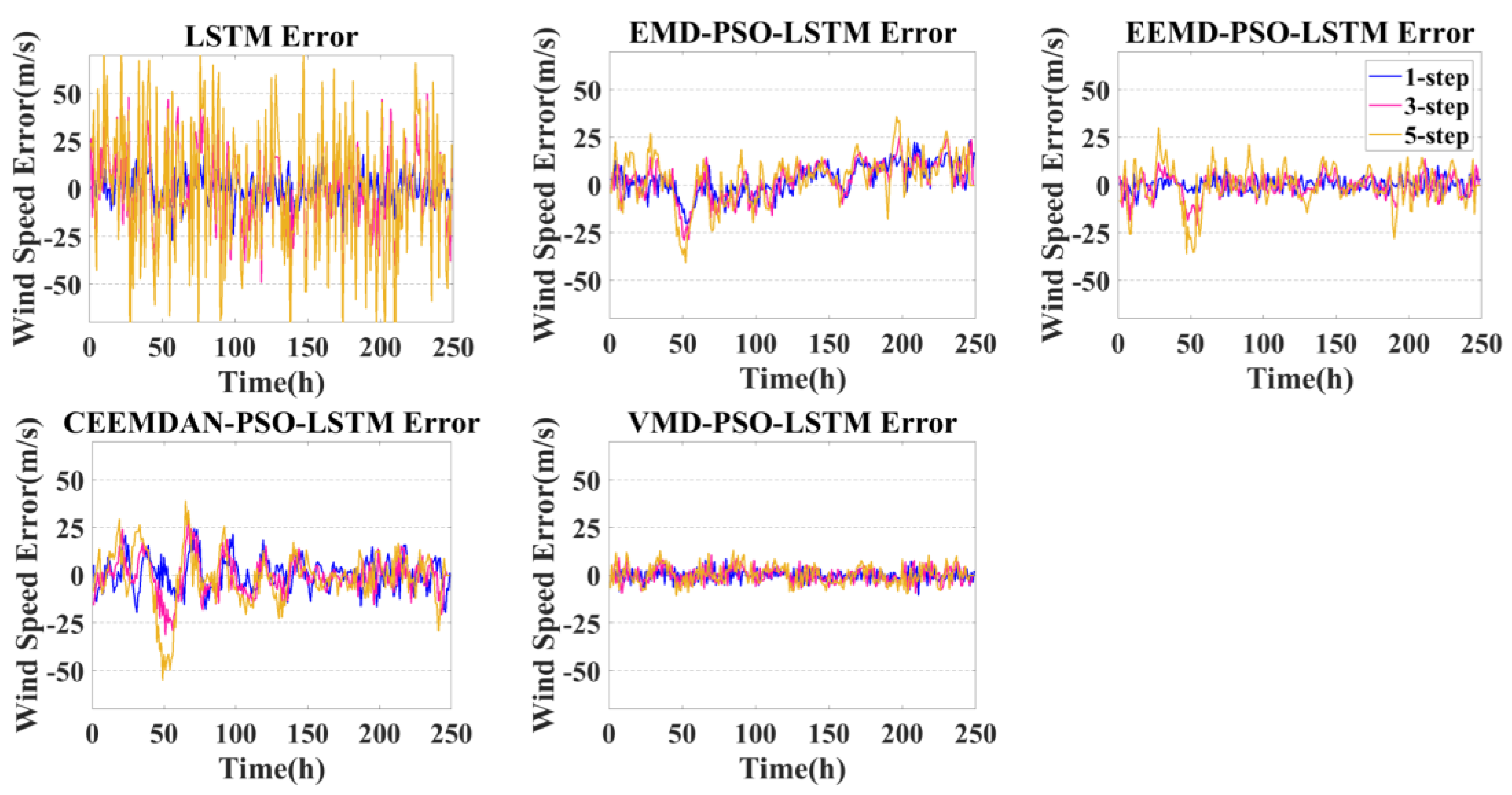
Considering the disadvantages of the poor prediction accuracy of traditional prediction models for the upper atmosphere in near space, the multimodal decomposition method and traditional prediction methods are analyzed and compared. Then, this paper describes a high-accuracy prediction model with a short term (VMD–PSO–LSTM). The VMD–PSO–LSTM prediction model can effectively reduce the impact of the dual characteristics of nonlinearity and non-stationarity in the wind speed series during the prediction performance. Further prediction experiments on the wind speed at 80–88 km altitude over Kunming led to the following meaningful conclusions.
  • The wind speed prediction at 80–88 km in the Kunming area shows that the multi-step prediction errors R M S E and M A P E of VMD–PSO–LSTM at all heights are less than 6 m/s and 15%, which proves that the method has good effectiveness and stability in predicting the atmospheric wind speed above 80 km in near space.
  • By analyzing several commonly used decomposition algorithms, VMD can better decompose nonstationary data into multiple smooth subseries, reduce the complexity of the data and improve the prediction accuracy.
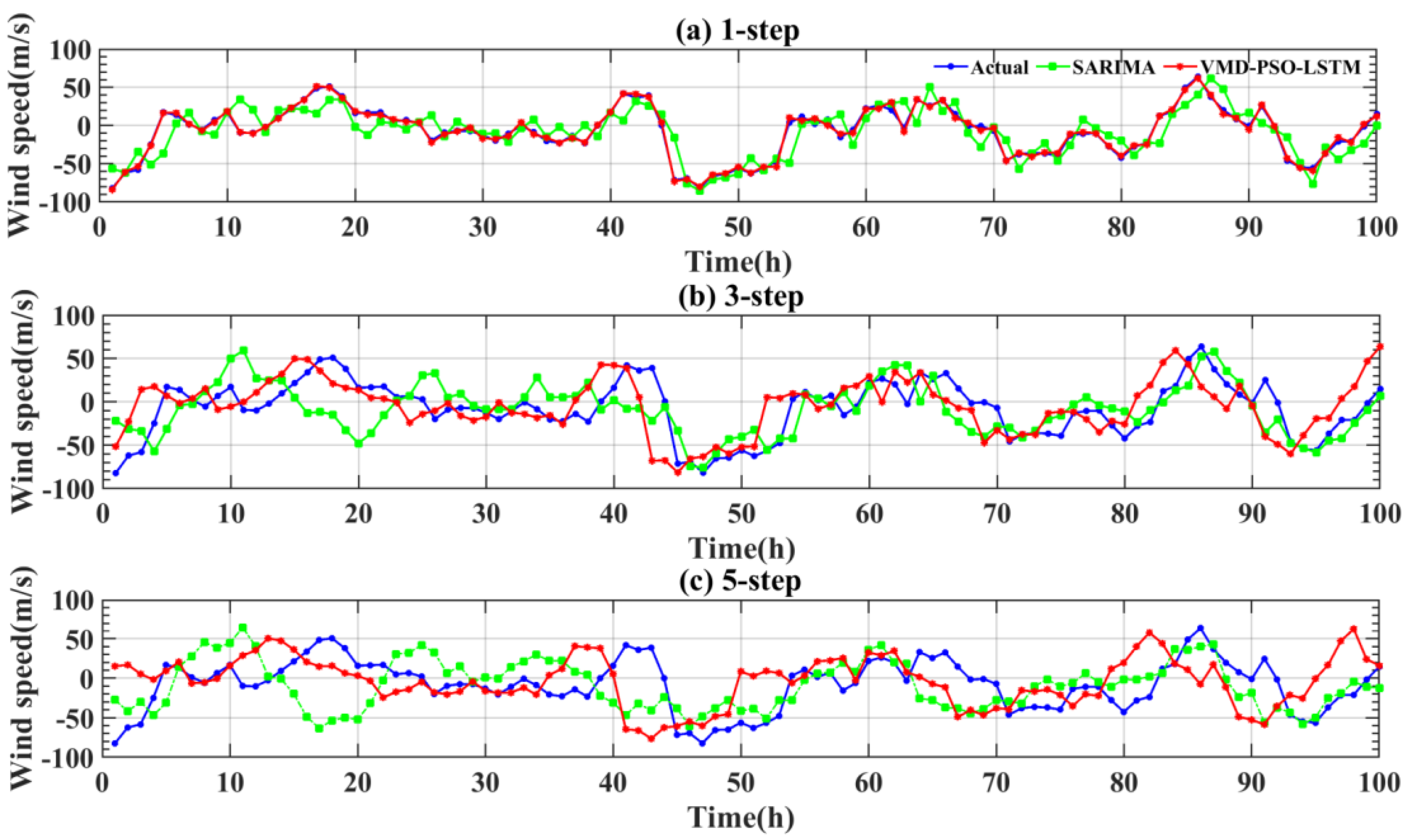
  • Compared with the traditional time series prediction model SARIMA, the hybrid prediction model VMD–PSO–LSTM has better prediction ability. The VMD–PSO–LSTM model not only solves the single-point lag problem of the traditional prediction method, but also improves the R M S E and M A P E relative to the traditional model by 85.21% and 83.75%, respectively.
  • The multi-step prediction results show that the prediction error increases with the increasing number of prediction steps. The main reason may be that the multi-step prediction strategy makes the input and output of the network model increase, and then the nonlinear relationship between the input data and the output data increases, which makes the function fitting more complicated. The result leads to the prediction value deviating from the true value with the growth of the prediction steps.
We can conclude that VMD–PSO–LSTM has more stable prediction performance than several other prediction models, and the VMD algorithm has better decomposition performance than several other algorithms. However, the model has some problems to be improved. The details are as follows.
First, in this paper, we use the central frequency observation method and empirical method to determine the decomposition layer K and penalty factor of VMD with some error and chance. There is no guarantee that the parameters determined are the optimal combination of parameters. Therefore, it is necessary to further study a more reasonable method to determine VMD parameters.
Second, this paper only considers the characteristics of wind field data itself for model prediction, without considering time, spatial latitude and other factors. Therefore, the next step of this paper is to consider the influence of various factors, such as time and space, on wind speed series prediction and establish a spatiotemporal network model with multifactor integration to further improve the accuracy of the prediction of atmospheric wind speed in near space.

Author Contributions

Conceptualization, S.Y. and N.L.; methodology, Z.D.; software, S.Y.; project administration, N.L.; supervision, N.L.; writing–original draft, S.Y., N.L. and H.Y.; funding acquisition, N.L. All authors have read and agreed to the published version of the manuscript.

Funding

This research was funded by the JKW Foundation, grant numbers 6142403210103 and 6142403200101 and A152001005.

Institutional Review Board Statement

Not applicable.

Informed Consent Statement

Not applicable.

Data Availability Statement

Not applicable.

Acknowledgments

The authors thank all the editors and reviewers for their valuable comments that greatly improved the presentation of this paper. The authors are very grateful to the China Research Institute of Radiowave Propagation for providing the data derived from the meteor radar in the Kunming area.

Conflicts of Interest

The authors declare no conflict of interest.

References

  1. Xiao, C.Y.; Hu, X.; Wang, B.; Yang, J.F. Quantitative studies on the variations of near space atmospheric fluctuation. Chin. J. Geophys. (Chin.) 2016, 59, 1211–1221. [Google Scholar]
  2. Li, N.; Chen, J.S.; Ding, Z.H.; Xu, Z.W.; Lin, L.K. Wind-oscillation Measurement and Study in Near Space. Equip. Environ. Eng. 2017, 14, 35–40. [Google Scholar]
  3. Yang, J.F.; Xiao, C.Y.; Hu, X.; Cheng, X. Wind shear characteristics in near space and their impacts on air vehicle. J. Beijing Univ. Aeronaut. Astronaut. 2019, 45, 57–65. [Google Scholar]
  4. Shi, Z.G.; Zhang, X.Q.; Li, J.T. Effect of ground pressure-maintenance index on stagnation performance of stratospheric aerostats. Acta Aeronaut. Astronaut. Sin. 2016, 37, 1833–1840. [Google Scholar]
  5. Long, Y.; Deng, X.L.; Yang, X.X.; Hou, Z.X. Short-term rapid prediction of stratospheric wind field based on PSO-BP neural network. J. Beijing Univ. Aeronaut. Astronaut. 2022, 48, 1970–1978. [Google Scholar]
  6. Cheng, C.; Wang, X.L. Thermal sensitivity factors analysis of stratospheric airships. J. Zhejiang Univ. (Eng. Sci.) 2020, 54, 202–212. [Google Scholar]
  7. Jiang, Z.Y.; Jia, Q.S.; Guan, X.H. A review of multi-temporal-and-spatial-scale wind power forecasting method. Acta Autom. Sin. 2019, 45, 51–71. [Google Scholar]
  8. Liu, T.; Xiao, C.Y.; Hu, X.; Tu, C.; Yang, J.F.; Xu, Q.C. Application of Time Series Method in Forecasting Near-space Atmospheric Windormalsize. J. Space Sci. 2018, 38, 211–220. [Google Scholar]
  9. Allen, D.R.; Coy, L.; Eckermann, S.D.; McCormack, J.P.; Manney, G.L.; Hogan, T.F.; Kim, Y.-J. NOGAPS-ALPHA simulations of the 2002 Southern Hemisphere stratospheric major warming. Mon. Weather. Rev. 2006, 134, 498–518. [Google Scholar] [CrossRef]
  10. Roney, J.A. Statistical wind analysis for near-space applications. J. Atmos. Sol.-Terr. Phys. 2007, 69, 1485–1501. [Google Scholar] [CrossRef]
  11. Xiao, C.Y.; Hu, X.; Yang, J.F.; Cheng, X. Aura/MLS Satellite Data Assimilation Technology and Its Application in Numerical Prediction in the near space. In Proceedings of the 4th China High Resolution Earth Observation Conference, Wuhan, China, 17–18 September 2017; pp. 30–46. [Google Scholar]
  12. Hu, X.; Gong, J.C.; Yang, J.F. A study of near-space atmospheric prediction methods. In Proceedings of the 3rd China High Resolution Earth Observation Conference, Beijing, China, 1 December 2014; pp. 290–299. [Google Scholar]
  13. He, W.H.; Wu, Y.J.; Deng, L.; Li, G.Q.; Wang, H.Y.; Tian, Y.; Ding, W.; Wang, W.H.; Xie, Y. Comparing SNNs and RNNs on neuromorphic vision datasets: Similarities and differences. Neural Netw. 2020, 132, 108–120. [Google Scholar] [CrossRef] [PubMed]
  14. Zhao, W.P.; Zhao, J.; Li, J.C.; Zhao, D.D.; Huang, L.L.; Zhu, J.X.; Lu, J.Z.; Wang, X. An Evaporation Duct Height Prediction Model Based on a Long Short-Term Memory Neural Network. IEEE Trans. Antennas Propag. 2021, 69, 7795–7804. [Google Scholar] [CrossRef]
  15. Dang, M.X.; Wu, J.J.; Cui, S.C.; Guo, X.; Cao, Y.H.; Wei, H.L.; Wu, Z.S. Multiscale Decomposition Prediction of Propagation Loss in Oceanic Tropospheric Ducts. Remote Sens. 2021, 13, 1173. [Google Scholar] [CrossRef]
  16. Mao, B.N.; Bu, Z.H.; Xu, B.; Gong, H.P.; Li, Y.; Wang, H.L.; Kang, J.; Jin, S.Z.; Zhao, C.L. Denoising method based on VMD-PCC in φ-OTDR system. Opt. Fiber Technol. 2022, 74, 103081. [Google Scholar] [CrossRef]
  17. Li, F.; Xiong, J.J.; Lan, X.H.; Bi, H.K.; Chen, X. NSHV trajectory prediction algorithm based on aerodynamic acceleration EMD decomposition. J. Syst. Eng. Electron. 2021, 32, 103–117. [Google Scholar]
  18. Dragomiretskiy, K.; Zosso, D. Variational mode decomposition. IEEE Trans. Signal Process. 2013, 62, 531–544. [Google Scholar] [CrossRef]
  19. Guo, F.; Deng, S.Y.; Zheng, W.J.; Wen, A.; Du, J.F.; Huang, G.S.; Wang, R.Y. Short-Term Electricity Price Forecasting Based on the Two-Layer VMD Decomposition Technique and SSA-LSTM. Energies 2022, 15, 8445. [Google Scholar] [CrossRef]
  20. Ji, H.; Yin, B.; Zhang, J.; Zhang, Y.; Li, Q.; Hou, C. Multiscale Decomposition Prediction of Propagation Loss for EM Waves in Marine Evaporation Duct Using Deep Learning. J. Mar. Sci. Eng. 2023, 11, 51. [Google Scholar] [CrossRef]
  21. Zhao, L.; Zhou, M.Y. A Robust Power Allocation Algorithm for Cognitive Radio Networks Based on Hybrid PSO. Sensors 2022, 22, 6796. [Google Scholar] [CrossRef] [PubMed]
  22. Wang, J.; Li, X.; Zhou, X.D.; Zhang, K. Ultra-short-term wind speed prediction based on VMD-LSTM. Power Syst. Prot. Control 2020, 48, 45–52. [Google Scholar]
  23. Zhi, L.H.; Zi, Y.; Xu, K. Combination prediction of wind speed based on variational mode decomposition and neural network. J. Hefei Univ. Technol. (Nat. Sci.) 2022, 45, 1505–1510+1584. [Google Scholar]
  24. Li, Z.Y.; Li, S.; Mao, J.D.; Li, J.; Wang, Q.; Zhang, Y. A Novel Lidar Signal-Denoising Algorithm Based on Sparrow Search Algorithm for Optimal Variational Modal Decomposition. Remote Sens. 2022, 14, 4960. [Google Scholar] [CrossRef]
  25. Song, X.; Liu, Y.; Xue, L.; Wang, J.; Zhang, J.; Wang, J.; Jiang, L.; Cheng, Z. Time-series well performance prediction based on Long Short-Term Memory (LSTM) neural network model. J. Pet. Sci. Eng. 2020, 186, 106682. [Google Scholar] [CrossRef]
  26. Song, G.; Zhang, Y.F.; Bao, F.X.; Qin, C. Stock prediction model based on particle swarm optimization LSTM. J. Beijing Univ. Aeronaut. Astronaut. 2019, 45, 2533–2542. [Google Scholar]
  27. Sun, Z.; Zhao, M.; Zhao, G. Hybrid model based on VMD decomposition, clustering analysis, long short memory network, ensemble learning and error complementation for short-term wind speed forecasting assisted by Flink platform. Energy. 2022, 261, 125248. [Google Scholar] [CrossRef]
  28. Du, B.G.; Huang, S.; Guo, J.; Tang, H.T.; Wang, L.; Zhou, S.W. Interval forecasting for urban water demand using PSO optimized KDE distribution and LSTM neural networks. Appl. Soft. Comput. 2022, 122, 108875. [Google Scholar] [CrossRef]
  29. Parasyris, A.; Alexandrakis, G.; Kozyrakis, G.V.; Spanoudaki, K.; Kampanis, N.A. Predicting Meteorological Variables on Local Level with SARIMA, LSTM and Hybrid Techniques. Atmosphere 2022, 13, 878. [Google Scholar] [CrossRef]
  30. Haddad, M.; Nicod, J.; Mainassara, Y.B.; Rabehasaina, L.; Al Masry, Z.; Péra, M. Wind and solar forecasting for renewable energy system using sarima-based model. In Proceedings of the International Conference on Time Series and Forecasting, Gran Canaria, Spain, 25–27 September 2019. [Google Scholar]
  31. Yi, W.; Chen, J.S.; Ma, C.B.; Li, N.; Zhao, Z.W. Observation of upper atmospheric temperature by Kunming all-sky meteor radar. Chin. J. Geophys. (Chin.) 2014, 57, 2423–2432. [Google Scholar]
  32. Chen, J.S.; Xu, L.L.; Ma, C.B.; Li, N.; Lin, L.K. A new method of determining momentum flux based on the all-sky meteor radar. Chin. J. Radio Sci. 2016, 31, 1124–1131. [Google Scholar]
  33. Zhou, B.Z.; Chen, J.S.; Li, Q.L.; Li, N.; Tang, Y. A new method of measuring neutral atmospheric density in the upper mesosphere. Chin. J. Radio Sci. 2017, 32, 687–693. [Google Scholar]
  34. Yi, W.; Xue, X.; Chen, J.; Dou, X.; Chen, T.; Li, N. Estimation of mesopause temperatures at low latitudes using the Kunming meteor radar. Radio Sci. 2016, 51, 130–141. [Google Scholar] [CrossRef]
  35. Yi, W.; Reid, I.M.; Xue, X.; Younger, J.P.; Spargo, A.J.; Murphy, D.J.; Chen, T.; Dou, X. First observation of mesosphere response to the solar wind high-speed streams. J. Geophys. Res. Space Phys. 2017, 122, 9080–9088. [Google Scholar] [CrossRef]
  36. Holdsworth, D.A.; Reid, I.M. Comparisons of full correlation analysis (FCA) and imaging Doppler interferometry (IDI) winds using the Buckland Park MF radar. Ann. Geophys. 2004, 22, 3829–3842. [Google Scholar] [CrossRef]
  37. Lee, C.; Kim, J.-H.; Jee, G.; Lee, W.; Song, I.-S.; Kim, Y.H. New method of estimating temperatures near the mesopause region using meteor radar observations. Geophys. Res. Lett 2004, 43, 10580–10585. [Google Scholar] [CrossRef]
  38. Liu, L.; Liu, H.; Le, H.; Chen, Y.; Sun, Y.; Ning, B.; Hu, L.; Wan, W.; Li, N.; Xiong, J. Mesospheric temperatures estimated from the meteor radar observations at Mohe. J. Geophys. Res. Space Phys. 2017, 122, 2249–2259. [Google Scholar] [CrossRef]
  39. Lu, X.; Yang, C.; Wu, Q.; Wang, J.; Lu, Z.; Sun, S.; Liu, K.; Shao, D. Research on Analog Circuit Soft Fault Diagnosis Method Based on Mathematical Morphology Fractal Dimension. Electronics 2023, 12, 184. [Google Scholar] [CrossRef]
  40. Fan, W.; He, Y.Z.; Wang, Y.; Chen, H. Early unbalance fault diagnosis on the exciting force of a linear vibrating screen based on VMD-RQA. J. Vib. Con. 2021, 40, 25–32. [Google Scholar]
  41. Yuan, J.J.; Luo, R.B.; Liao, J.; Yang, Z.C.; Wang, N.; Li, J. Application of Three Neural Network Models in the Prediction of Stratospheric Wind Field. High Power Convert. Technol. 2019, 05, 12–16. [Google Scholar]
  42. Qiao, S.; Wang, L.; Zhang, P.C.; Yan, Q.M.; Wang, G.B. Short-term Load Forecasting by Long- and Short-term Temporal Networks with Attention Based on Modal Decomposition. Power Syst. Technol. 2022, 46, 3940–3951. [Google Scholar]
  43. Chen, H.; Bu, Y.; Zong, K.; Huang, L.; Hao, W. The Effect of Data Skewness on the LSTM-Based Mooring Load Prediction Model. J. Mar. Sci. Eng. 2022, 10, 1931. [Google Scholar] [CrossRef]
  44. Wang, D.; Cui, X.; Niu, D. Wind Power Forecasting Based on LSTM Improved by EMD-PCA-RF. Sustainability 2022, 14, 7307. [Google Scholar] [CrossRef]
Figure 1. The overall flowchart of the VMD−PSO−LSTM model. From top to bottom are data preprocessing, decomposition algorithm, prediction model, prediction reorganization and model evaluation.
Atmosphere 14 00315 g001
Figure 2. Data preprocessing flow chart. The x_train is the training set data and the y_train is the label of the x_train. The x_test is the test set data and the y_test is the label of the x_test.
Atmosphere 14 00315 g002
Figure 3. PSO–LSTM model algorithm flowchart. Finding parameters (batch size, epoch, learning rate) of LSTM network structure by particle swarm algorithm.
Atmosphere 14 00315 g003
Figure 4. IMF components of wind speed sequence for the 86 km zonal wind (K = 9). The IMFs diagram are shown on the (left), and the center frequency corresponding to the IMFs are shown on the (right).
Atmosphere 14 00315 g004
Figure 5. VMD–PSO–LSTM zonal wind 80–88 km prediction results from 14–23 June 2019. From top to bottom are observations, predicted value and absolute errors.
Atmosphere 14 00315 g005
Figure 6. VMD–PSO–LSTM meridional wind 80–88 km prediction results from 14–23 June 2019. From top to bottom are observations, predicted value and absolute errors.
Atmosphere 14 00315 g006
Figure 7. Normalization results of meridional wind at 86 km from 1 May to 23 June 2019.
Atmosphere 14 00315 g007
Figure 8. Comparison results of different decomposition prediction models (14–23 June 2019), observations (black line), one-step predicted value (blue line), three-step predicted value (red line) and five-step predicted value (green line).
Atmosphere 14 00315 g008
Figure 9. Error results for different decomposition prediction models (14–23 June 2019), one-step prediction error (blue line), three-step prediction error (red line) and five-step prediction error (yellow line).
Atmosphere 14 00315 g009
Figure 10. Comparison of SARIMA and VMD–PSO–LSTM prediction results, observations (blue line), SARIMA predicted value (green line) and VMD–PSO–LSTM predicted value (red line).
Atmosphere 14 00315 g010
Table 1. The ST Kunming meteor radar main operating parameters.
ParameterValue
Transmitter operating frequency53.1 MHz
pulse repetition frequency430 Hz
peak output power40 kw
correlation stack4
distance precision1.8 km
pulse typeGaussian pulse
detection range70–110 km
Table 2. Central frequency for the IMF components of the 86 km zonal wind.
KIMF1IMF2IMF3IMF4IMF5IMF6IMF7IMF8IMF9IMF10IMF11IMF12
40.0007 0.0468 0.1805 0.3022
50.0005 0.0410 0.0811 0.1304 0.3032
60.0005 0.0408 0.0800 0.1203 0.1956 0.3054
70.0005 0.0407 0.0809 0.1186 0.1667 0.2474 0.4226
80.0005 0.0397 0.0624 0.0883 0.1706 0.3073 0.3993 0.4786
90.0005 0.0396 0.0602 0.0841 0.1179 0.1701 0.2416 0.3313 0.4554
100.0005 0.0396 0.0604 0.0842 0.1167 0.1627 0.2190 0.2989 0.3708 0.4524
110.0005 0.0396 0.0604 0.0842 0.1194 0.1656 0.2179 0.2881 0.3403 0.3958 0.4552
120.0004 0.0396 0.0594 0.0824 0.1000 0.1250 0.1619 0.1966 0.2461 0.3099 0.3807 0.4555
Table 3. Best number of decompositions for 80–88 km meridional and zonal wind sequences.
HeightZonal WindMeridional Wind
Best Number of DecompositionsBest Number of Decompositions
80 km1011
82 km1210
84 km1010
86 km98
88 km99
Table 4. Results of hyperparameters optimized by PSO based on 86 km zonal wind.
86 km Zonal WindBatch_SizeEpochLearning Rate
IMF1142260.0092
IMF2161950.0087
IMF3132890.0098
IMF4261690.0073
IMF5332470.0067
IMF6172150.0089
IMF7213360.0097
IMF8133370.0093
IMF9192380.0086
Table 5. VMD–PSO–LSTM prediction errors at different heights.
HeightZonal WindMeridional Wind
Predicted Steps R M S E M A P E   ( % ) Predicted Steps R M S E M A P E   ( % )
80 km12.076.7611.204.13
33.5811.7832.739.44
54.2413.5253.5811.36
82 km11.604.5712.548.14
32.708.2933.5511.45
52.938.9255.2614.92
84 km12.216.5412.176.49
33.4310.0633.7510.83
54.1111.8154.6614.72
86 km11.113.4013.299.67
32.236.9334.3712.93
53.059.4055.1314.40
88 km12.487.5512.286.99
33.359.8334.7213.14
54.1713.2755.2614.59
Table 6. Evaluation metrics for different decomposition prediction models.
ModelPredicted Steps R M S E M A P E   ( % )
LSTM18.82426.01
310.4430.6
515.5244.04
EMD–PSO–LSTM18.825.6
39.629.4
513.4438.25
EEMD–PSO–LSTM13.559.94
36.117.18
57.8324.83
CEEMDAN–PSO–LSTM18.6423.6
39.925.7
514.736.41
VMD–PSO–LSTM13.289.46
34.1612.19
55.0614.13
Table 7. SARIMA and VMD–PSO–LSTM model evaluation index results.
Evaluation IndicatorsPredicted StepsSARIMAVMD–PSO–LSTM
R M S E 119.383.28
330.204.16
534.695.06
M A P E (%)143.809.46
368.5312.19
588.6014.13
P R M S E 1/83.02%
3/85.52%
5/85.21%
P M A P E 1/77.92%
3/81.13%
5/83.75%
Disclaimer/Publisher’s Note: The statements, opinions and data contained in all publications are solely those of the individual author(s) and contributor(s) and not of MDPI and/or the editor(s). MDPI and/or the editor(s) disclaim responsibility for any injury to people or property resulting from any ideas, methods, instructions or products referred to in the content.

