1. Introduction
Quantitative studies in climate science involve various functional relations. They may include the statistically established relations, e.g., the prediction of precipitation with preceding sea surface temperature and snow cover over the Tibetan Plateau, along with other possible factors. The functional relations include the physical laws, e.g., the equation of state for ideal dry gas, which provides a linkage among atmospheric pressure, density, and temperature. The functional relations may also include those that are mathematically defined based on physical considerations, e.g., the link of relative humidity with atmospheric water vapor and air temperature.
These functional relations can be classified into two types. One is the causal relation, in which a dependent quantity is affected by two or more independent variables, as in the example of using sea surface temperature and the snow cover over the plateau to predict the precipitation. The other type is the constraint relation. As a simultaneous relation, it includes three or more variables in an equation. There is no causality, and all the variables are equal in position. The ideal gas law is an example of this type. The relation of relative humidity, water vapor, and air temperature can be treated as a causal relation when examining how water vapor and air temperature influence relative humidity. It may also be treated as a constraint relation, as in meteorological calculation when computing one of the humidity quantities with the data of the other two variables.
Dominance analysis [
1,
2] can be performed with quantitative relations to better understand the corresponding issues. For causal relations, we can compare the relative contributions from the independent variables to the variation of the dependent quantity and identify which variable is more important to the variation. Lu et al. [
3] studied the interannual variations of streamflow and other hydrological components and examined whether precipitation or temperature, the two input climate variables, dominates the variations. Lu et al. [
4] investigated the interannual variation of the seasonal rainfall total, with different thresholds for defining the precipitation and explored whether the number of rainy days or the averaged rainfall intensity dominates the variation. Precipitation can be affected by changes in atmospheric water vapor and air temperature, which can both be influenced by atmospheric circulation. Tu and Lu [
5] revealed whether the change in water vapor or the change in air temperature is more important to the interannual variation of seasonal precipitation. Derivation shows that the atmospheric static stability is a function of air temperature and its vertical difference. Lu et al. [
6] provided the results of whether temperature or the vertical difference of temperature is more important to the seasonal, interannual, and spatial variations of the static stability. In the present study, we turn to examining the constraint relation. As an example, here we consider the ideal gas law [
7] and investigate the pertinent dominance issues.
Broadly speaking, all quantitative relations can be treated as nonlinear relations. For the dominance analysis, it would be convenient if the relations can be linearized. With observed data, statistical fitting can be used to obtain the linear relations. Significance tests are required to ensure the robustness of the linearization. Previous studies showed that for many of the problems examined, statistical fittings could well linearize the corresponding relations [
1,
2,
3,
4,
5,
6,
8]. For the different causal relations, the independent variables are regressed with respect to the dependent quantity [
3,
4,
5,
6]. In this study, for the constraint relation, the linearization of the relation will be performed by using the plane equation fitting [
9,
10,
11,
12,
13], in which the noise may come from all the variables. The advantage of the plane equation is that the relation fitted can cover all the situations, including those degenerate cases, i.e., the special cases with the simplified relations being between different pairs of the variables.
In the fitted plane equation, the dominance can be examined by using the “scale analysis”, which is a powerful tool in mathematical sciences for simplifying equations that contain multiple terms [
14,
15,
16,
17,
18]. The method has conventionally been used in dynamic meteorology for analyzing the balance equations, such as the conservations in momentum, mass, and energy [
19,
20,
21]. In the present study, through linearization, we establish a balance equation that has three terms. Because of the normalizations, the changes of the different variables can be compared. The scales of the three terms can be measured simply with the three coefficients contained in the linearized equation. For this specific gas law issue, a linearized relation can be obtained from both statistical fitting and analytical derivation.
With the balance equation of the three terms, the dominance analysis includes two aspects. One is simplifying the equation. With neglecting the term that is smallest in scale, the equation can be simplified as a rough balance between the other two terms. The three types of the simplifications can reflect the three ideal gas laws, that is, Charle’s law, which states that when pressure does not change, the density is inversely proportional to temperature [
22], Boyle’s law, with temperature remaining unchanged and density being proportional to pressure [
23], and Gay-Lussac’s law, in which density is constant while pressure is proportional to the temperature [
24]. The other aspect of dominance analysis is to locate the dominant quantity when examining the variation of the term that is smallest in scale. The term is a residual between the two larger terms. The largest term dominates the variation, while the second largest term exerts a negative effect on the variation. For the different dominance types and patterns, their geographical preferences are revealed in this study.
The equation of state for ideal dry air provides a nonlinear and simultaneous multivariate relation. The physical relation of the three quantities, as an equation, is simple in form. While we determine the dominance quantitative by use of the calculation approach, we may also deduce the dominance analytically from the original physical relation. Thus, their results can be compared. This is the reason why we deliberately choose the ideal gas law as the example for the dominance analysis. The comparison demonstrates that the approach used for the study is reliable.
Atmospheric pressure, temperature, and density are important climate quantities. They can both influence and be influenced by the atmospheric circulation. The spatial inhomogeneity of the pressure, as well as the high and low pressure systems, can affect the regional and large-scale circulations [
25,
26,
27,
28]. The horizontal difference of air temperature may lead to thermal wind and jet streams [
29,
30,
31,
32]. The temporal–spatial variations of the air density may relate to the convergence of the air parcel and then the wind energy, the gravity waves, and the greenhouse temperature [
33,
34,
35,
36,
37]. In this study, we focus on the interannual variations of the near-surface atmosphere.
The NCEP/NCAR Reanalysis I [
38], provided by the National Centers for Environmental Prediction (NCEP) and the National Center for Atmospheric Research (NCAR), is used in this study. The data used include the monthly surface air temperature and pressure, with a horizontal resolution of 2.5° × 2.5° in latitude and longitude over the 71 years from 1948 to 2018. The monthly surface air density is then calculated with the ideal gas law.
The main goal of the present study is to raise the question, propose the method, and take the state equation of dry air near surface as an example to locate the regions, over the globe where the relation of the three quantities is dominated by the different types and patterns. In
Section 2, plane equation fitting is applied, as for the general nonlinear problem, to linearize the relation. In addition, for this special problem, the gas law, the linear relation is also obtained from the derivation. In
Section 3, we assess the relative importance for each pair of the quantities through comparing their coefficients obtained in the linearized relation. In
Section 4, comparisons are further performed among the three coefficients to display the regional patterns for the dominance. The scale analysis tool is introduced to simplify the three-quantity equation and determine the dominant relation and the dominant quantity. An example is provided in
Section 5, for the most common pattern, to present the details pertinent to the coefficients and the scales and the correlations and the normalizations, as well as the balance of the terms in the equation and their interannual variations. A summary and discussion are given in
Section 6.
3. The Comparisons between Each Pair of the Coefficients
Figure 3 shows the distributions of the ratios
,
, and
for the six months. The plots of
illustrate the relative importance of the temperature and density in the covariations. At most grid points in the globe,
AD is larger than
BT throughout the year, especially at the belts over the mid-high-latitude oceans in the two hemispheres. Thus, density is more important than temperature in the covariations. However, in some areas, e.g., Central Africa, northern Eurasia, the Tibetan Plateau, the West Coast of North America, Greenland, and Antarctica, the
BT in some months can be larger than
AD, thus temperature is more important than density. The spatial pattern of the
also has seasonal shifts, and this is mainly due to the significant seasonal shifts of the
BT, along with the smaller seasonal changes in the
AD.
The plots of compare the contributions of density and pressure. The AD is larger than CP in most regions over the globe, especially over the lands and the tropical and subtropical oceans, throughout the year. Hence, overall density is more important than pressure in the covariations. The plots of compare the contributions of temperature and pressure. The general spatial pattern of is similar with that of . The difference is that in the plots of , there are large areas where CP is larger, e.g., over the mid-high-latitude oceans in the two hemispheres. This may be associated with the storm track in the middle latitudes, where the variations in pressure are relatively large, while sea surface temperature (and hence surface air temperature) varies rather little. In both the plots of and , seasonal shifts can be noticed for the belts in the two hemispheres, where correspondingly, the C is larger.
4. Scale Analysis of the Balance Equation and Regional Dominance of the Relation
4.1. The Scales and Dominance Issues for the Three-Quantity Equation
Scale analysis, or the order–of–magnitude analysis, is a useful tool for the simplification of an equation that contains multiple terms. It first approximates the magnitude of each individual term in the equation and then neglects some small terms and thus simplifies the equation. The scale analysis method has been applied in dynamical meteorology to simplify balance equations, such as conservation equations [
27]. The method is used to simplify the equation that contains at least three terms or for three variables [
14].
Consider the three-term equation. For simplicity, the equation can be expressed as , where the three terms S, M, and N are all positive. Rewrite the equation as . What the three-term equation implies is a balance of the larger term S by the two smaller terms M and N. Here, S is greater than both M and N in magnitude. By using the concept of scale analysis, it can be termed as “the scale of the S is larger than the scales of the M and N”. With mathematic notation, this can be written as and . In the present study, we examine the following two issues for the dominance in the three-term equation.
One is to find the dominant relation by simplifying the equation. Assume that M is much greater than N in magnitude, i.e., . Then, we may ignore the small term N and simplify the equation of the three terms as , a relation that describes a rough balance between the two dominant terms, the S and M. The other is to locate the dominant quantity when it is required to examine the variation of the smallest term N. Rewrite the equation as . The N is a residual between S and M, the two larger terms. Here, the S has a positive effect and thus dominates the variation of the N. The M has a negative effect on the variation. For the specific issue of the relation of density, temperature, and pressure in this study, the differences of the magnitudes of AD, BT, and CP may not be very large everywhere over the globe. However, the scale analysis is still pretty useful.
4.2. The Six Dominance Patterns and Their Geographical Preferences
In
Section 3, for each pair of the quantities, the magnitudes of the corresponding terms in the equation are compared. The comparisons are all over the entire field. However, in different regions, the balance relation of the three terms may be dominated by different pairs of the quantities. In some regions, the relation can be simplified as the balance between density and temperature, while in other regions, the relation may be dominated by the balance between density and pressure or by the balance between temperature and pressure. Here, for each grid point, we use the scale analysis introduced above to conduct the dominance examinations, i.e., to find the local relation dominated by two major quantities and their relative importance to the variation of the third quantity.
For examining the dominance, we may have three types (and further six patterns) through comparing the values of
AD,
BT, and
CP.
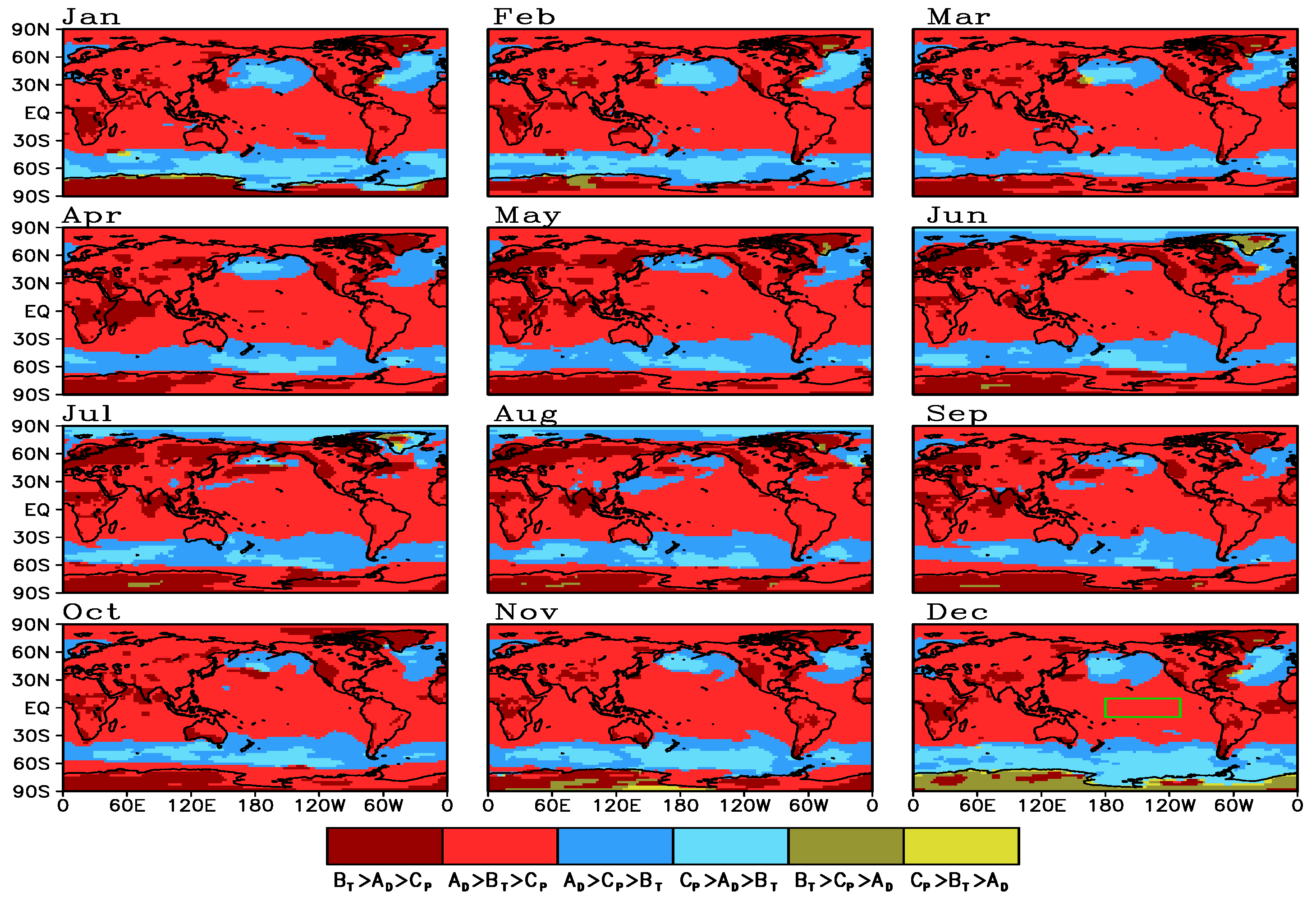
Figure 4 shows the spatial distributions of these types and patterns. The three types are classified in terms of the smallest coefficient, from the
AD,
BT, and
CP. In
Figure 4, the grid points with the
CP being the smallest, with the
BT being the smallest, and with the
AD being the smallest are marked in red, blue, and yellow, respectively. For each type, we may further divide it into two patterns in terms of the comparison of the other two coefficients. For example, for the type in red, with the
CP being the smallest, the grid points are further divided into the pattern with
, which is marked in dark red, and the pattern with
, which is marked in light red. The overall spatial distributions of these patterns for all the months in
Figure 4 suggest that the patterns for the dominance possess significant geographical preferences.
Table 1 presents the percentages of the grid points for the six patterns and the ratios of the grid points to the total over the globe. The percentages are provided for all the months, and their averages are used to assess the overall situation for the patterns. Over most grid points in the globe (75.7%; red), the type is the one with
CP being the smallest. Among them, the most popular pattern is the one with
(61.5%; light red). Inside the wide regions of this pattern (
Figure 4), there are some areas with the pattern of
(14.2%; dark red). There is also a considerable number of grid points (23.1%; blue) where the type is the one with
BT being the smallest. They are mainly over the mid-high-latitude oceans in the two hemispheres. Within these regions, there are areas with the pattern of
(15.5%; dark blue) and areas with the pattern of
(7.6%; light blue). The grid points for the third type with
AD being the smallest (1.3%; yellow) are less and are major as the pattern of
(1.1%; dark yellow). This pattern occurs mainly over Greenland in June and over Antarctica in December.
For each of the six patterns, the scale analysis method can be applied to examine the two dominance issues. In the fitted plane equation , as mentioned above, because of the normalizations, the three quantities D, T, and P are all in the magnitude of one. Or the scales of the three quantities are all equal to one, and this can be denoted as . Then, the scales of the three terms AD, BT, and CP can be represented by the corresponding coefficients A, B, and C. With the notation, this can be expressed as , , and .
For the most common pattern with
, which prevails over the wide regions marked in light red in
Figure 4, the scale of the
CPP is the smallest of the three terms. Actually, over these regions, the
AD and
BT are both much greater than the
CP in most of the grid points, as reflected in the plots of the
and
in
Figure 3. That is,
and
. As the first issue for the dominance, we may ignore the term
CPP and simplify the equation as
, representing a rough balance between the terms of the density and temperature. It can be inferred from this dominant relation that the
D and
T are negatively correlated. This means that corresponding to a larger-than-normal density, there might be a lower-than-normal temperature. As the second issue for the dominance, when examining the variation of the pressure, we rewrite the equation as
. This suggests that the small term
CPP is the residual (i.e., the difference) between the two larger terms
ADD and −
BTT. For this pattern with the
, we can also infer from the rewritten equation that the
D is positively correlated with the
P and thus dominates its variation. The
T is negatively correlated with the
P and has a negative effect on its variation.
The two patterns with the BT being the smallest of the three, which appear over the northern Pacific, the northern Atlantic, and the ocean belt north of Antarctica, are also important. Similar to the above analysis, we may ignore the term BTT, and simplify the relation as , a rough balance between pressure and density. The D and P may have a positive correlation. For the pattern with , with the equation being rewritten as , the term BTT can be treated as the residual between the terms CPP and ADD. Thus, pressure dominates the variation of the temperature, and density has a negative effect. For the pattern with , we rewrite the equation as , and the term BTT can be regarded as the residual between the terms ADD and CPP. The variation of temperature is dominated by its negative correlation with density, i.e., the decrease in density, although the positive correlation with pressure can have a positive effect on the variation.
The AD can also be the smallest of the three, and this is mainly for the pattern with . This pattern appears mainly over Greenland in June and Antarctica in December. With neglecting the ADD and simplifying the equation as , the balance is between temperature and pressure. For the variation, we rewrite the equation as and conclude that the ADD is the residual between the terms BTT and CPP. The variation of density is dominated by its negative correlation with temperature, i.e., the decrease in temperature, although the positive correlation with pressure can have a positive effect on the variation.
5. An Example with More Details from the Most Common Pattern
The most common pattern, with
, is taken as an example in this section. In the plot of December in
Figure 4, a region with this pattern is selected and marked in green. The region lies in the central equatorial Pacific (110° W–180° W, 10° S–10° N). The pressure and temperature are averaged over the region. The density for the region is then calculated with the gas law. The plane fitting is performed for this region.
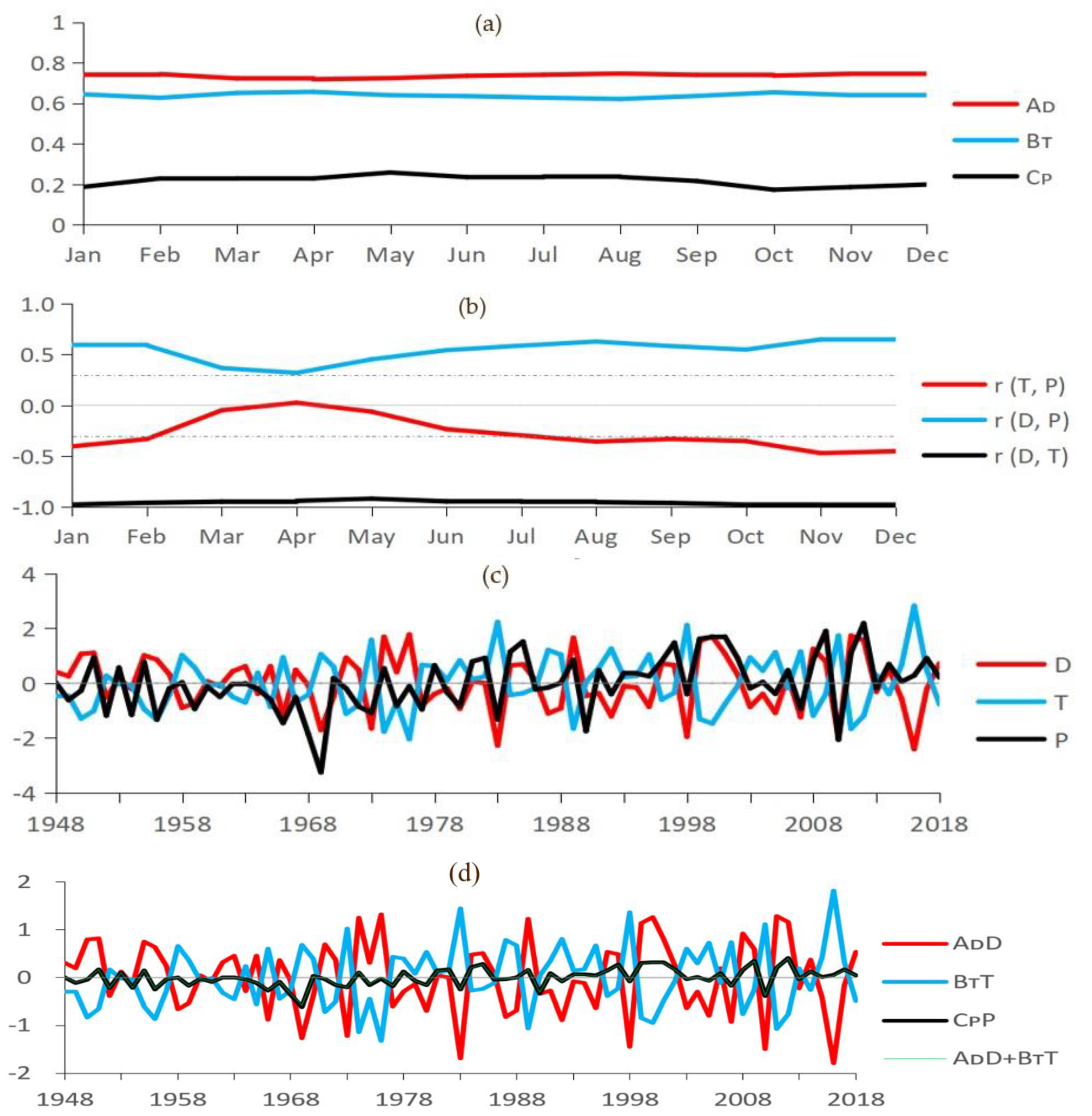
Figure 5 presents some more details of the pattern for the linear fitting, the scale analysis, and the results of the dominance.
Figure 5a presents the coefficients
AD,
BT, and
CP obtained for each month. Their values are pretty stable over the months. The
AD and
BT are comparable and large, while relatively the
CP is rather small. Thus, in the three-term equation, we may neglect the
CPP and simplify the relation as a rough balance between the terms
ADD and
BTT, i.e.,
. It can be inferred that
D and
T have different signs, suggesting that density and temperature are negatively related.
Figure 5b shows that the correlation between
D and
T is truly negative, and it is very strong. The correlation coefficient can be almost −1.0 for all the months.
For examining the variation of the pressure, we rewrite the equation as
. Comparison shows that
AD is greater than
BT in all months (
Figure 5a). For a positive
CPP in a year, we may infer from the equation that the
ADD is positive, while the
BTT is negative. This is consistent with the calculated results in
Figure 5b, which indicates that pressure has a positive correlation with density but has a negative correlation with temperature. The
CPP is thus a residual (or difference) between the two terms
ADD and −
BTT. So, for this pattern, density dominates the variation of the pressure. Because of the dominance, the positive correlation of the pressure and density is strong. In contrast, temperature has a negative effect on the variation of the pressure.
With January being an example,
Figure 5c displays the interannual variations of the three normalized quantities
D,
T, and
P. They all have large year-to-year variations, and they are all in the magnitude of one because of the normalizations. Hence, the scales of the three terms
ADD,
BTT, and
CPP can be measured simply with the corresponding coefficients
AD,
BT, and
CP. In addition, the curves can reflect the very strong negative correlation between the
D and
T, as well as the strong positive correlation between the
P with
D.
Figure 5d shows the interannual variations of the
ADD,
BTT, and
CPP, as well as the
. Here, the
CPP corresponds to the pressure observed, and the
is the
CPP calculated with the fitted plane equation. In the plot, the curves of the
CPP and the
coincide exactly. This confirms the conclusion that for the gas law, a nonlinear relation, the plane fitting adopted in this study is perfect in linearizing the relation. We then may utilize the scale analysis method to assess the terms in the balance equation. The year-to-year perturbations of the
ADD and
BTT are truly large in scale, but they are opposite in sign. The
CPP or the
is small in scale and reflects the net effects of the terms
ADD and
BTT. The
ADD is greater than
BTT in magnitude, thus
ADD dominates the variation of the
CPP, and
BTT has a negative effect on the variation.
6. Conclusions and Discussion
Dominance analysis is usually performed for the causal relation to find out the relative importance of the independent quantities to the dependent quantity. In this study, we examine the constraint relation with no causality and try to understand the dominance patterns in the relation.
Pressure, temperature, and density are important quantities for diagnosing the atmospheric circulation and the climate. For dry ideal gas, they are nonlinearly linked as the gas law. The relation is a simultaneous constraint. Although the three quantities are equal in position and they may all have changes regionally because of the interactions in the climate system, it is possible that one quantity does not change much, and the relation can be simplified as a balance between the other two quantities. In some regions, the relation may become Charle’s law, with the density and temperature being inversely correlated. Over other regions, the relation may tend to be Boyle’s law, with density and pressure being positively correlated, or Gay-Lussac’s law, with temperature and pressure being positively correlated.
To be convenient for assessing the dominance, it is better to linearize the original nonlinear relation. For a general nonlinear problem, we use statistical fitting to linearize the relation. With the normalized quantities D, T, and P, the fitted plane equation can be expressed as , where , and . Statistical tests indicate that the linearization is robust. Results show that corresponding to , the coefficients AD and BT are both positive everywhere. For this specific nonlinear problem, the gas law, the linearized relation can also be obtained from analytical derivations. Comparison indicates that the results are the same.
Scale analysis is a useful tool for simplifying equations that contain multiple terms. It has been applied in dynamical meteorology for analyzing conservation equations. Here, in the equation , because of the normalizations, the quantities D, T, and P are all in the magnitude of one. So, the D, T, and P are actually the “dimensionless” variables for density, temperature, and pressure. Then, the coefficients AD, BT, and CP can be regarded as the “scales” of the three quantities. Through comparing the scales, we examine two issues for the regional dominance. The first is to simplify the equation. After finding the smallest of the three scales, we may ignore the term and retain the other two terms in the equation. The second is to examine the variation of this term, which is the smallest in scale. The other two terms are opposite in sign but comparable in magnitude. Thus, the small-scale term we examine is a residual between the two large-scale terms. One of them dominates the variation, and the other has a negative effect on the variation.
For the dominance analysis, three types (and six further patterns) are obtained through comparing the three coefficients AD, BT, and CP. The geographical distributions of the six patterns are provided for each of the months. The most common pattern is the one with (e.g., over the central equatorial Pacific), which appears over 60% of the grid points in the globe. The CP is the smallest coefficient. In most of the regions, the CP is actually much smaller than the AD and BT. So, in the equation, we may ignore the CPP, and simplify the equation as . It is inferred that the D and T are opposite in sign and negatively correlated. When examining the variation of the pressure, we rewrite the equation as . Since , it can also be inferred that ADD has a positive correlation with CPP and thus dominates the variation of the CPP. The BTT has a negative effect on the variation. Hence, the CPP is a residual (or difference) between the terms ADD and −BTT.
For the type with CP being the smallest coefficient, another pattern is the one with , which appears mainly over some land areas within the wide regions of the above pattern. The type with BT being the smallest coefficient appears over the mid-high-latitude oceans in the two hemispheres. In the equation, we may ignore the BTT and simplify it as , suggesting a balance between the terms of pressure and density. The D and P can be positively correlated. The variation of the BTT can be analyzed with the equation . This type contains two patterns. For the pattern with , the D and T are negatively correlated, and −ADD dominates the variation of BTT, while CPP has a negative effect. For the pattern with , CPP dominates the variation of BTT, and −ADD has a negative effect on the variation. The type with AD being the smallest coefficient, especially the pattern with , may appear over some land areas in some months.
The example for the most common pattern displays many details on the plane fitting and the scale analysis. The quantitative results from this case examination are consistent with the results qualitatively inferred above from the fitting and the scale analysis. For instance, for this pattern with , the linear fitting is perfect. The year-to-year curve of CPP from the observation and the curve of CPP from the fitted equation coincide exactly. The coefficients AD and BT are comparable, and they are truly much larger than the CP. The normalized D, T, and P all have large interannual variations, although all in magnitude of one. The D and T have very strong negative correlation. The variation of the pressure is truly dominated by density, and the effect of temperature is negative.
For the linearized equation , it is displayed that the spatial patterns of BT and CP, the scales of the terms of temperature and pressure, have significant seasonal shifts. The belts with small values of BT and the belts with large values of CP, which are over mid-high-latitude oceans in the two hemispheres, move northwards during the first half of the year and southwards in the second half. This may be related to the seasonal movements of the incident solar radiation between the northern and southern hemispheres. This may be related to the storm tracks being located at slightly lower latitudes in winter than in summer. However, the spatial pattern of the AD, the scale of the term of density, does not change much seasonally. Further investigations will be conducted to better understand these.
The task of the present study is to raise the question, propose the method, and locate the regions over the globe where the relation of the three quantities is dominated by the different types and patterns. It is the major finding of this study that the different dominance types and patterns have their geographical preferences. The two patterns with the CP being the smallest of the three appear over most of the regions in the globe. The patterns with the BT being the smallest appear over the northern Pacific, the northern Atlantic, and the ocean belt north of Antarctica. The patterns with the AD being the smallest appear mainly over Greenland in June and Antarctica in December.
Atmospheric dynamics and physics will be investigated in our future work for the different types or patterns of the dominance in the relation. They are the final regional display, resulting from the dynamics and physics, as well as the interactions among the quantities. The investigation may also include the large-scale atmospheric circulation. This study needs to be conducted, individually, for each of the regions. The pattern, for example, appears over many land areas, including Antarctica, the Tibetan Plateau, South Africa, Eurasia, Greenland, and West America. For this pattern, the questions we may examine include why the variations of the temperature and density can offset each other and why the variation of the pressure is dominated by temperature rather than density. For the different land areas, the atmospheric circulation and physical processes responsible for the two questions can be different. For the pattern , which only appears over Greenland in June and Antarctica in December, we may examine to find out what is special in the corresponding atmospheric circulations.
Water vapor is also an important quantity in real atmosphere. The relation among the pressure, temperature, density, and relative humidity (or other quantity that indicate moisture) is much more complex. The effect of the moisture will also be investigated in our future work. As a first step, we focus on the dry air in the present study and examine the dominance among pressure, temperature, and density, the three quantities for the dry air. We will consider the moist air through introducing a moisture quantity and then compare the relative importance of the moisture quantity with the dry-air quantities. Over the different regions of different dominance patterns, we may identify whether the variation of the moisture can be more important than the variations of the dry-air quantities or one or two of them.


