
Vehicle Pollutant Dispersion in the Urban Atmospheric Environment: A Review of Mechanism, Modeling, and Application
Abstract
:1. Introduction
2. Research Methods for Urban Vehicle Pollutant Dispersion Mechanism
2.1. Field Measurement
2.2. Wind Tunnel Experiment
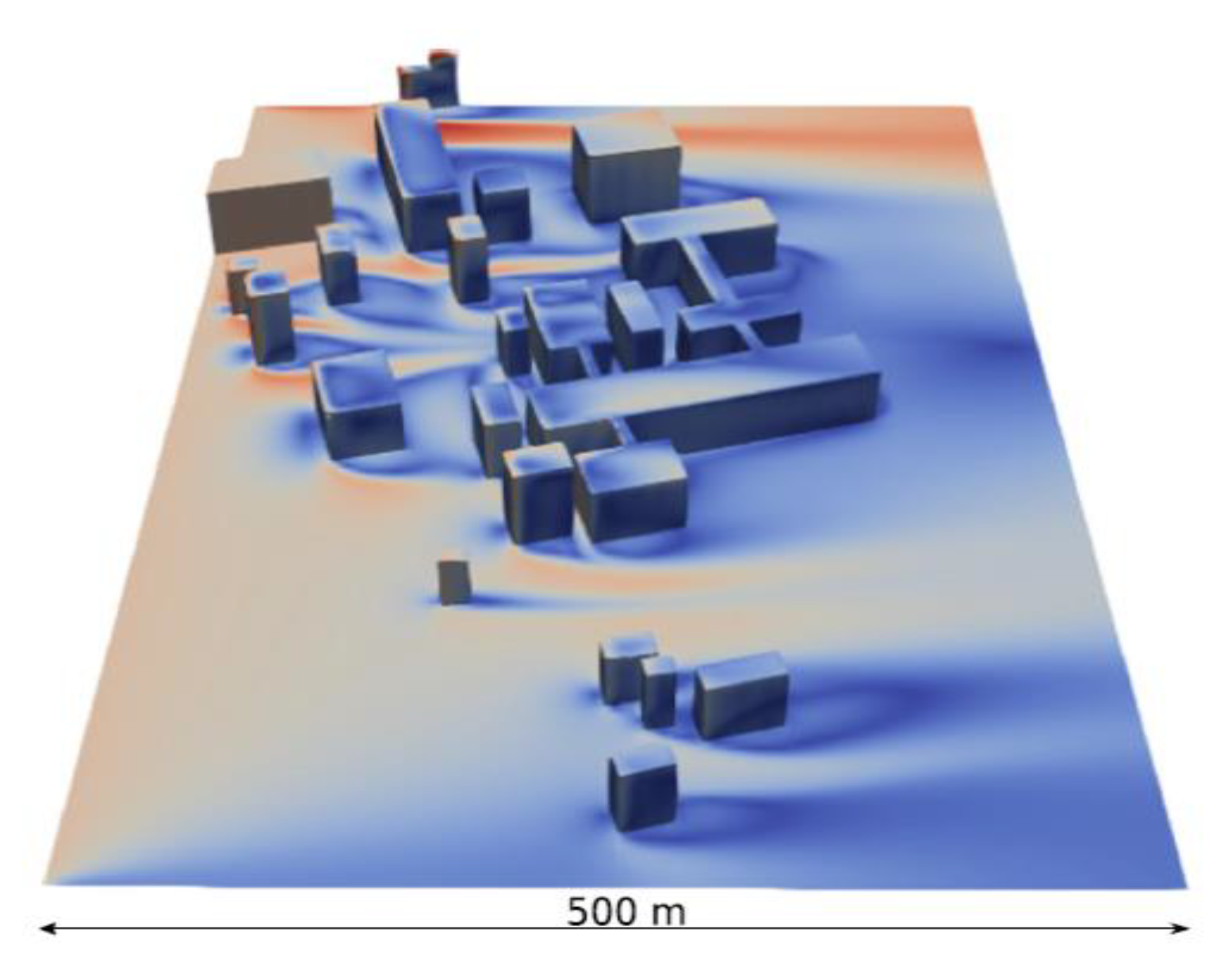
2.3. Numerical Simulation
3. Urban Vehicle Pollutant Dispersion Models
3.1. Box Model
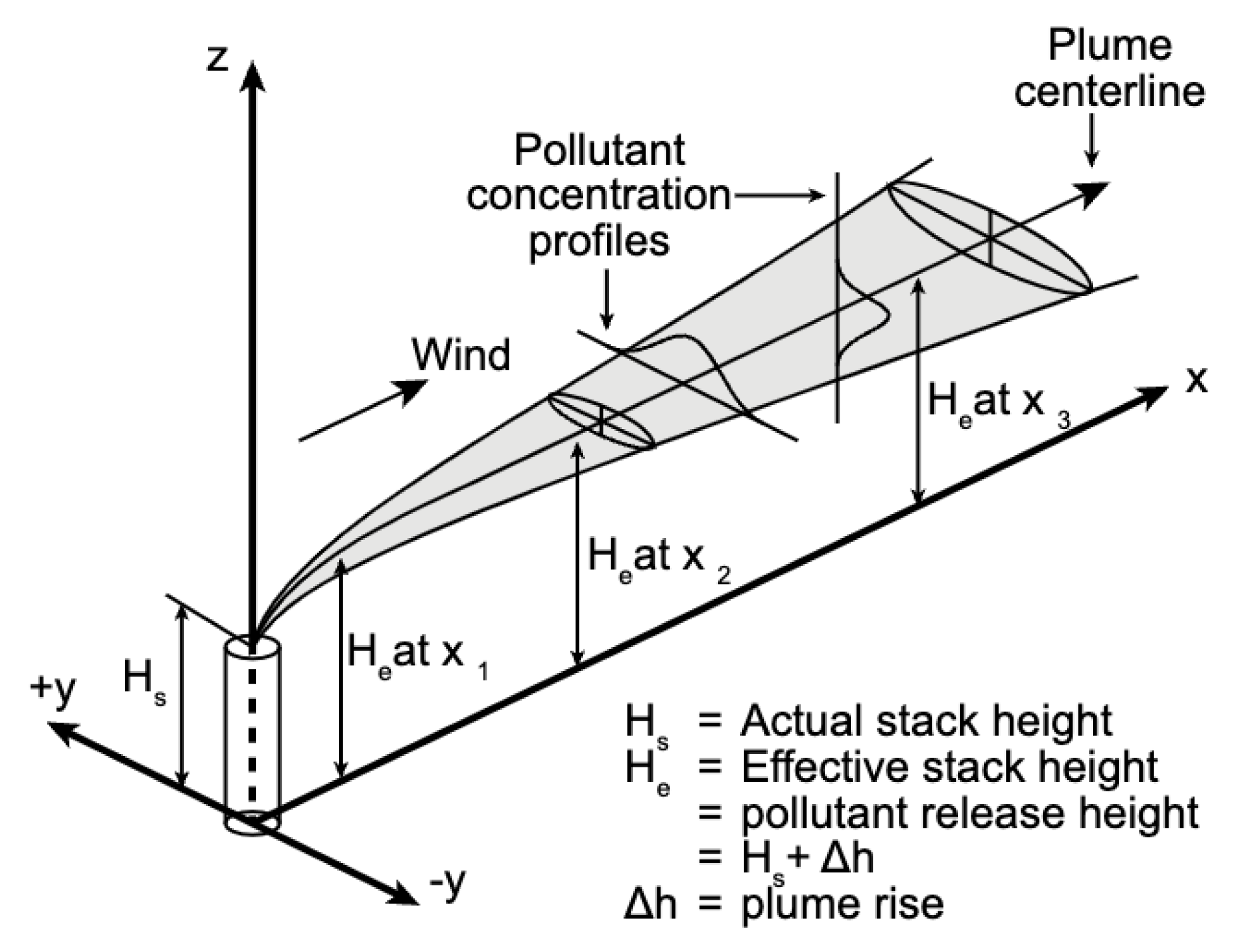
3.2. Gaussian Model
3.2.1. Classical Street-Emission Dispersion Models
3.2.2. Urban-Scale Systematic Models
3.2.3. Street-Network Models
4. Conclusions
Author Contributions
Funding
Institutional Review Board Statement
Informed Consent Statement
Data Availability Statement
Acknowledgments
Conflicts of Interest
References
- Tu, Y.; Xu, C.; Wang, W.; Wang, Y.; Jin, K. Investigating the impacts of driving restriction on NO2 concentration by integrating citywide scale cellular data and traffic simulation. Atmos. Environ. 2021, 265, 118721. [Google Scholar] [CrossRef]
- Xu, T.; Barman, S.; Levin, M.W.; Chen, R.; Li, T. Integrating public transit signal priority into max-pressure signal control: Methodology and simulation study on a downtown network. Transp. Res. Part C Emerg. Technol. 2022, 138, 103614. [Google Scholar] [CrossRef]
- Xu, T.; Levin, M.W.; Cieniawski, M. A Zone-Based Dynamic Queueing Model and Maximum-Stability Dispatch Policy for Shared Autonomous Vehicles. In Proceedings of the 2021 IEEE International Intelligent Transportation System Conference (ITSC), Indianapolis, IN, USA, 19–22 September 2021; pp. 3827–3832. [Google Scholar]
- Tu, Y.; Wang, W.; Li, Y.; Xu, C.; Xu, T.; Li, X. Longitudinal safety impacts of cooperative adaptive cruise control vehicle’s degradation. J. Saf. Res. 2019, 69, 177–192. [Google Scholar] [CrossRef] [PubMed]
- Forehead, H.; Huynh, N. Review of modeling air pollution from traffic at street-level. State Sci. Environ. Pollut. 2018, 241, 775–786. [Google Scholar] [CrossRef] [PubMed]
- Fallah-Shorshani, M.; Shekarrizfard, M.; Hatzopoulou, M. Evaluation of regional and local atmospheric dispersion models for the analysis of traffic-related air pollution in urban areas. Atmos. Environ. 2017, 167, 270–282. [Google Scholar] [CrossRef]
- De Visscher, A. Air Dispersion Modeling: Foundations and Applications; John Wiley & Sons: Hoboken, NJ, USA, 2013. [Google Scholar]
- Leelőssy, Á.; Molnár, F.; Izsák, F.; Havasi, Á.; Lagzi, I.; Mészáros, R. Dispersion modeling of air pollutants in the atmosphere: A review. Open Geosci. 2014, 6, 257–278. [Google Scholar] [CrossRef]
- Wedding, J.B.; Lombardi, D.J.; Cermak, J.E. A wind tunnel study of gaseous pollutants in city street canyons. J. Air. Pollut. Control. Assoc. 1977, 27, 557–566. [Google Scholar] [CrossRef]
- Kadaverugu, R.; Sharma, A.; Matli, C.; Biniwale, R. High resolution urban air quality modeling by coupling CFD and mesoscale models: A review. Asia-Pac. J. Atmos. Sci. 2019, 55, 539–556. [Google Scholar] [CrossRef]
- Kono, H.; Ito, S. A micro-scale dispersion model for motor vehicle exhaust gas in urban areas—OMG volume-source model. Atmos. Environ. Part B. Urban Atmos. 1990, 24, 243–251. [Google Scholar] [CrossRef]
- Lee, I.Y.; Park, H.M. Comparison of microphysics parameterizations in a three-dimensional dynamic cloud model. Atmos. Environ. 1994, 28, 1615–1625. [Google Scholar] [CrossRef]
- Sini, J.F.; Anquetin, S.; Mestayer, P.G. Pollutant dispersion and thermal effects in urban street canyons. Atmos. Environ. 1996, 30, 2659–2677. [Google Scholar] [CrossRef]
- Meroney, R.; Ohba, R.; Leitl, B.; Kondo, H.; Grawe, D.; Tominaga, Y. Review of CFD guidelines for dispersion modeling. Fluids 2016, 1, 14. [Google Scholar] [CrossRef]
- Chang, C.H.; Meroney, R.N. Numerical and physical modeling of bluff body flow and dispersion in urban street canyons. J. Wind Eng. Ind. Aerodyn. 2001, 89, 1325–1334. [Google Scholar] [CrossRef] [Green Version]
- Kim, J.J.; Baik, J.J. A numerical study of the effects of ambient wind direction on flow and dispersion in urban street canyons using the RNG k–ε turbulence model. Atmos. Environ. 2004, 38, 3039–3048. [Google Scholar] [CrossRef]
- Salim, S.M.; Buccolieri, R.; Chan, A.; Sabatino, S.D. Numerical simulation of atmospheric pollutant dispersion in an urban street canyon: Comparison between RANS and LES. J. Wind Eng. Ind. Aerodyn. 2011, 99, 103–113. [Google Scholar] [CrossRef]
- Živković, P. Air Quality Estimation and Error Analysis. Innov. Mech. Eng. 2022, 1, 30–42. [Google Scholar]
- Ehm, C.; Frohmüller, M.O.; Flassak, T.; Stephan, D. On-site reduction of nitrogen oxides at an emission hotspot using actively vented photocatalytic reactors in a highway tunnel. SN Appl. Sci. 2022, 4, 153. [Google Scholar] [CrossRef]
- Qin, H.; Hong, B.; Jiang, R. Are green walls better options than green roofs for mitigating PM10 pollution? CFD simulations in urban street canyons. Sustainability 2018, 10, 2833. [Google Scholar] [CrossRef] [Green Version]
- Sun, D.J.; Wu, S.; Shen, S.; Xu, T. Simulation and assessment of traffic pollutant dispersion at an urban signalized intersection using multiple platforms. Atmos. Pollut. Res. 2021, 12, 101087. [Google Scholar] [CrossRef]
- Lauriks, T.; Longo, R.; Baetens, D.; Derudi, M.; Parente, A.; Bellemans, A.; van Beeck, J.; Denys, S. Application of improved CFD modeling for prediction and mitigation of traffic-related air pollution hotspots in a realistic urban street. Atmos. Environ. 2021, 246, 118127. [Google Scholar] [CrossRef]
- Aris, M.H.M.; Darlis, N.; Ishak, I.A.; Sulaiman, S.; Jaat, N.; Hakim, A.F. HVAC CFD Analysis of Air Flow and Temperature Distribution Inside Passenger Compartment. J. Automot. Powertrain Transp. Technol. 2021, 1, 25–33. [Google Scholar]
- Hasan, A.; ElGammal, T.; Amano, R.S.; Khalil, E.E. Flow Patterns and Temperature Distribution in an Underground Metro Station. Energy Sustainability. Am. Soc. Mech. Eng. 2018, 51418, V001T06A004. [Google Scholar]
- Li, J.; Yu, Y.; Wang, Y.; Zhao, L.; He, C. Prediction of Transient NOx Emission from Diesel Vehicles Based on Deep-Learning Differentiation Model with Double Noise Reduction. Atmosphere 2021, 12, 1702. [Google Scholar] [CrossRef]
- Kumar, P.; Ketzel, M.; Vardoulakis, S.; Pirjola, L.; Britter, R. Dynamics and dispersion modeling of nanoparticles from road traffic in the urban atmospheric environment—A review. J. Aerosol Sci. 2011, 42, 580–603. [Google Scholar] [CrossRef] [Green Version]
- Johnson, W.B.; Ludwig, F.L.; Dabberdt, W.F.; Allen, R. An urban diffusion simulation model for carbon monoxide. Air Pollut. Control Assoc. 1973, 23, 490–498. [Google Scholar] [CrossRef] [PubMed]
- Nicholson, S.E. A pollution model for street-level air. Atmos. Environ. (1967) 1975, 9, 19–31. [Google Scholar] [CrossRef]
- Yamartino, R.J.; Wiegand, G. Development and evaluation of simple models for the flow, turbulence and pollutant concentration fields within an urban street canyon. Atmos. Environ. (1967) 1986, 20, 2137–2156. [Google Scholar] [CrossRef]
- Hotchklss, R.S.; Harlow, F.H. Air Pollution Transport M Street Canyons; United States Environmatal Protection Agency: Wasington, DC, USA, 1973; EPA-R4-73-029. [Google Scholar]
- Sobottka, H. Air Pollution Impact in Streets with Heavy Traffic and the Effects of the Dominant Parameters. In Studies in Environmental Science; Elsevier: Amsterdam, The Netherlands, 1980; Volume 8, pp. 109–114. [Google Scholar]
- Gualtieri, G. A street canyon model intercomparison in Florence, Italy. Water Air Soil Pollut. 2010, 212, 461–482. [Google Scholar] [CrossRef]
- Mensink, C.; Colles, A.; Janssen, L.; Cornelis, J. Integrated air quality modeling for the assessment of air quality in streets against the council directives. Atmos. Environ. 2003, 37, 5177–5184. [Google Scholar] [CrossRef]
- Lefebvre, W.; Vercauteren, J.; Schrooten, L.; Janssen, S.; Degraeuwe, B.; Maenhaut, W.; de Vlieger, I.; Vankerkom, J.; Cosemans, G.; Mensink, C.; et al. Validation of the MIMOSA-AURORA-IFDM model chain for policy support: Modeling concentrations of elemental carbon in Flanders. Atmos. Environ. 2011, 45, 6705–6713. [Google Scholar] [CrossRef]
- Beckx, C.; Panis, L.I.; Van De Vel, K.; Arentze, T.; Lefebvre, W.; Janssens, D.; Wets, G. The contribution of activity-based transport models to air quality modeling: A validation of the ALBATROSS–AURORA model chain. Sci. Total Environ. 2009, 407, 3814–3822. [Google Scholar] [CrossRef] [PubMed]
- US EPA. A Comparison of Calpuff Modeling Results to Two Tracer Field Experiments [EB/OL]. 1998. Available online: http://www.epa.gov/scram001/7thconf/calpuff/tracer.pdf. (accessed on 20 November 2022).
- Wikimedia Commons Contributors, "File:Gaussian Plume (SVG).svg," Wikimedia Commons, the Free Media Repository. 2020. Available online: https://commons.wikimedia.org/w/index.php?title=File:Gaussian_Plume_(SVG).svg&oldid=495553766 (accessed on 20 November 2022).
- Holmes, N.S.; Morawska, L. A review of dispersion modeling and its application to the dispersion of particles: An overview of different dispersion models available. Atmos. Environ. 2006, 40, 5902–5928. [Google Scholar] [CrossRef] [Green Version]
- Petersen, W.B. User’s Guide for HIWAY-2: A Highway Air Pollution Model; US Environmental Protection Agency: Washington, DC, USA, 1980. [Google Scholar]
- Benson, P.E. Caline 4-A Dispersion Model for Predicting Air Pollutant Concentrations Near Roadways; Transportation Research Board: Washington, DC, USA, 1984. [Google Scholar]
- Kenty, K.L.; Poor, N.D.; Kronmiller, K.G.; McClenny, W.; King, C.; Atkeson, T.; Campbell, S.W. Application of CALINE4 to roadside NO/NO2 transformations. Atmos. Environ. 2007, 41, 4270–4280. [Google Scholar] [CrossRef]
- Dhyani, R.; Sharma, N. Sensitivity analysis of CALINE4 model under mix traffic conditions. Aerosol Air Qual. Res. 2017, 17, 314–329. [Google Scholar] [CrossRef] [Green Version]
- Sharma, N.; Gulia, S.; Dhyani, R.; Singh, A. Performance evaluation of CALINE 4 dispersion model for an urban highway corridor in Delhi. J. Sci. Ind. Res. 2013, 72, 521–530. [Google Scholar]
- Broderick, B.M.; Budd, U.; Misstear, B.D.; Ceburnis, D.; Jennings, S. Validation of CALINE4 modeling for carbon monoxide concentrations under free-flowing and congested traffic conditions in Ireland. Int. J. Environ. Pollut. 2005, 24, 104–113. [Google Scholar] [CrossRef]
- Marmur, A.; Mamane, Y. Comparison and evaluation of several mobile-source and line-source models in Israel. Transp. Res. Part D Transp. Environ. 2003, 8, 249–265. [Google Scholar] [CrossRef]
- Hertel, O.; Berkowicz, R.; Larssen, S. The operational street pollution model (OSPM). In Air Pollution Modeling and Its Application VIII; Springer: Boston, MA, USA, 1991; pp. 741–750. [Google Scholar]
- Berkowicz, R. OSPM-A parameterized street pollution model. Environ. Monit. Assess. 2000, 65, 323–331. [Google Scholar] [CrossRef]
- Kukkonen, J.; Valkonen, E.; Walden, J.; Koskentalo, T.; Aarnio, P.; Karppinen, A.; Berkowicz, R.; Kartastenpää, R. A measurement campaign in a street canyon in Helsinki and comparison of results with predictions of the OSPM model. Atmos. Environ. 2001, 35, 231–243. [Google Scholar] [CrossRef]
- Kakosimos, K.E.; Hertel, O.; Ketzel, M.; Berkowicz, R. Operational Street Pollution Model (OSPM)—A review of performed application and validation studies, and future prospect. Environ. Chem. 2010, 7, 485–503. [Google Scholar] [CrossRef]
- Ketzel, M.; Jensen, S.S.; Brandt, J.; Ellermann, T.; Olesen, H.R.; Berkowicz, R.; Hertel, O. Evaluation of the street pollution model OSPM for measurements at 12 streets stations using a newly developed and freely available evaluation tool. J. Civ. Environ. Eng. 2012, S1, 004. [Google Scholar] [CrossRef] [Green Version]
- Allwine, K.J.; Dabberdt, W.F.; Simmons, L.L. Peer Review of the CALMET/CALPUFF Modeling System; EPA Contract No. 68-D-98-092; The KEVRIC Company Inc.: Durham, North Carolina, 1998. Available online: http://www.epa.gov/ttn/scram/7thconf/calpuff/calpeer.pdf. (accessed on 20 November 2022).
- Holnicki, P.; Kałuszko, A.; Trapp, W. An urban scale application and validation of the CALPUFF model. Atmos. Pollut. Res. 2016, 7, 393–402. [Google Scholar] [CrossRef]
- Elbir, T. Comparison of model predictions with the data of an urban air quality monitoring network in Izmir, Turkey. Atmos. Environ. 2003, 37, 2149–2157. [Google Scholar] [CrossRef]
- Barna, M.G.; Gimson, N.R. Dispersion modeling of a wintertime particulate pollution episode in Christchurch, New Zealand. Atmos. Environ. 2002, 36, 3531–3544. [Google Scholar] [CrossRef]
- Ivančič, M.; Vončina, R. Determinating the influence of different PM10 sources on air quality in Ljubljana basin with CALPUFF dispersion model. Int. J. Environ. Pollut. 2014, 54, 251–261. [Google Scholar] [CrossRef]
- Trapp, W. The application of CALMET/CALPUFF models in air quality assessment system in Poland. Arch. Environ. Prot. 2010, 36, 63–79. [Google Scholar]
- Joo, S.; Oh, C.; Lee, S.; Lee, G. Assessing the impact of traffic crashes on near freeway air quality. Transp. Res. Part D Transp. Environ. 2017, 57, 64–73. [Google Scholar] [CrossRef]
- Cimorelli, A.J.; Perry, S.G.; Venkatram, A.; Weil, J.C.; Paine, R.J.; Wilson, R.B.; Lee, R.F.; Peters, W.D.; Brode, R.W. AERMOD: A dispersion model for industrial source applications. Part I: General model formulation and boundary layer characterization. J. Appl. Meteorol. 2005, 44, 682–693. [Google Scholar] [CrossRef]
- Misra, A.; Roorda, M.J.; MacLean, H.L. An integrated modeling approach to estimate urban traffic emissions. Atmos. Environ. 2013, 73, 81–91. [Google Scholar] [CrossRef] [Green Version]
- Michelle, G.S.; Akula, V.; David, K.H.; Perry, S.G.; Petersen, W.B.; Isakov, V. RLINE: A line source dispersion model for near-surface releases. Atmos. Environ. 2013, 77, 748–756. [Google Scholar]
- Valencia, A.; Venkatram, A.; Heist, D.; Carruthers, D.; Arunachalam, S. Development and evaluation of the R-LINE model algorithms to account for chemical transformation in the near-road environment. Transp. Res. Part D Transp. Environ. 2018, 59, 464–477. [Google Scholar] [CrossRef] [PubMed] [Green Version]
- Dixon, J.; Middleton, D.R.; Derwent, R.G. Sensitivity of nitrogen dioxide concentrations to oxides of nitrogen controls in the United Kingdom. Atmos. Environ. 2001, 35, 3715–3728. [Google Scholar] [CrossRef]
- Hess, G.; Cope, M. A note on subgrid-scale processes in photochemical modelling. Atmos. Environ. 1989, 23, 2857–2860. [Google Scholar] [CrossRef]
- McHugh, C.A.; Carruthers, D.J.; Edmunds, H.A. Adms and adms–urban. Int. J. Environ. Pollut. 1997, 8, 438–440. [Google Scholar]
- Carruthers, D.J.; Holroyd, R.J.; Hunt, J.C.R.; Weng, E.S.; Robins, A.G.; Apsley, D.D.; Thompson, D.J.; Smith, F.B. UK-ADMS: A new approach to modeling dispersion in the earth’s atmospheric boundary layer. J. Wind Eng. Ind. Aerodyn. 1994, 52, 139–153. [Google Scholar] [CrossRef]
- ADMS—Urban C, U. ADMS—Roads and the latest government guidance. In UK Tools for Modelling NOX and NO2. ADMS—Urban and Roads User Group Meeting; CERC: Cambridge, UK, 2009. [Google Scholar]
- Hirtl, M.; Baumann-Stanzer, K. Evaluation of two dispersion models (ADMS-Roads and LASAT) applied to street canyons in Stockholm, London and Berlin. Atmos. Environ. 2007, 41, 5959–5971. [Google Scholar] [CrossRef]
- CERC. ADMS-Roads: An Air Quality Management System, User Guide Version 3.1.; CERC: Cambridge, UK, 2011. [Google Scholar]
- McHugh, C.A.; Carruthers, D.J.; Edmunds, H.A. ADMS–Urban: An air quality management system for traffic, domestic and industrial pollution. Int. J. Environ. Pollut. 1997, 8, 666–674. [Google Scholar]
- Stocker, J.; Hood, C.; Carruthers, D.; McHugh, C. ADMS–Urban: Developments in modelling dispersion from the city scale to the local scale. Int. J. Environ. Pollut. 2012, 50, 308. [Google Scholar] [CrossRef]
- Vijay, P.; Nagendra, S.M.; Gulia, S.; Khare, M.; Bell, M.; Namdeo, A. Performance Evaluation of UK ADMS-Urban Model and AERMOD Model to Predict the PM 10 Concentration for Different Scenarios at Urban Roads in Chennai, India and Newcastle City, UK. In Urban Air Quality Monitoring, Modelling and Human Exposure Assessment; Springer: Singapore, 2021; pp. 169–181. [Google Scholar]
- Badamfirooz, J.; Rahmati, A.; Daneshpajooh, N.; Mousazadeh, R.; Mirzaei, R. Investigating the impact of existing and under construction industries on the air quality of Arak City using ADMS model. Environ. Sci. 2021, 20, 21–40. [Google Scholar] [CrossRef]
- Rizza, V.; Torre, M.; Tratzi, P.; Fazzini, P.; Tomassetti, L.; Cozza, V.; Naso, F.; Marcozzi, D.; Petracchini, F. Effects of deployment of electric vehicles on air quality in the urban area of Turin (Italy). J. Environ. Manag. 2021, 297, 113416. [Google Scholar] [CrossRef]
- Ellis, K.; McHugh, C.; Carruthers, D.; Stidworthy, A. Comparison of ADMS-Roads, CALINE4 and UK DMRB Model Predictions for Roads; CERC Documentation: Cambridge, UK, 2001. [Google Scholar]
- Righi, S.; Lucialli, P.; Pollini, E. Statistical and diagnostic evaluation of the ADMS-Urban model compared with an urban air quality monitoring network. Atmos. Environ. 2009, 43, 3850–3857. [Google Scholar] [CrossRef]
- Hamer, P.D.; Walker, S.E.; Sousa-Santos, G.; Vogt, M.; Vo-Thanh, D.; Aparicio-Lopez, S.; Ramacher, M.O.P.; Karl, M. The urban dispersion model EPISODE. Part 1: A Eulerian and subgrid-scale air quality model and its application in Nordic winter conditions. Geosci. Model Dev. 2019, 13, 1–57. [Google Scholar]
- Karl, M.; Walker, S.E.; Solberg, S.; Ramacher, M.O. The Eulerian urban dispersion model EPISODE—Part 2: Extensions to the source dispersion and photochemistry for EPISODE–CityChem v1.2 and its application to the city of Hamburg. Geosci. Model Dev. 2019, 12, 3357–3399. [Google Scholar] [CrossRef] [Green Version]
- Soulhac, L.; Salizzoni, P.; Cierco, F.X.; Perkins, R. The model SIRANE for atmospheric urban pollutant dispersion; part I, presentation of the model. Atmos. Environ. 2011, 45, 7379–7395. [Google Scholar] [CrossRef]
- Soulhac, L.; Salizzoni, P.; Mejean, P.; Didier, D.; Rios, I. The model SIRANE for atmospheric urban pollutant dispersion; PART II, validation of the model on a real case study. Atmos. Environ. 2012, 49, 320–337. [Google Scholar] [CrossRef]
- Soulhac, L.; Nguyen, C.V.; Volta, P.; Salizzoni, P. The model SIRANE for atmospheric urban pollutant dispersion. PART III: Validation against NO2 yearly concentration measurements in a large urban agglomeration. Atmos. Environ. 2017, 167, 377–388. [Google Scholar] [CrossRef]
- Kim, Y.; Wu, Y.; Seigneur, C.; Roustan, Y. Multi-scale modeling of urban air pollution: Development and application of a Street-in-Grid model (v1.0) by coupling MUNICH (v1.0) and Polair3D (v1.8.1). Geosci. Model Dev. 2018, 11, 611–629. [Google Scholar] [CrossRef] [Green Version]
- Kim, Y.; Lugon, L.; Maison, A.; Sarica, T.; Roustan, Y.; Valari, M.; Zhang, Y.; André, M.; Sartelet, K. MUNICH v2.0: A street-network model coupled with SSH-aerosol (v1.2) for multi-pollutant modelling. Geosci. Model Dev. 2022, 15, 7371–7396. [Google Scholar] [CrossRef]
- Lugon, L.; Vigneron, J.; Debert, C.; Chrétien, O.; Sartelet, K. Black carbon modeling in urban areas: Investigating the influence of resuspension and non-exhaust emissions in streets using the Street-in-Grid model for inert particles (SinG-inert). Geosci. Model Dev. 2021, 14, 7001–7019. [Google Scholar] [CrossRef]
- Gavidia-Calderón, M.; Ibarra-Espinosa, S.; Kim, Y.; Zhang, Y.; Andrade, M.D.F. Simulation of O3 and NOx in Sao Paulo street urban canyons with VEIN (v0.2.2) and MUNICH (v1.0). Geosci. Model Dev. Discuss. 2020, 14, 3251–3268. [Google Scholar] [CrossRef]
- Ibarra-Espinosa, S.; Ynoue, R.; O’Sullivan, S.; Pebesma, E.; Andrade, M.D.F.; Osses, M. VEIN v0.2.2: An R package for bottom-up Vehicular Emissions Inventories. Geosci. Model Dev. Discuss. 2018, 11, 2209–2229. [Google Scholar] [CrossRef] [Green Version]
- Chan, E.C.; Leitao, J.; Kerschbaumer, A.; Butler, T.M. Yeti 1.0: A generalized framework for constructing bottom-up emission inventory from traffic sources. Geosci. Model Dev. Discuss. 2022. [Google Scholar] [CrossRef]


| Acronyms | Associated Model |
|---|---|
| ADMS | Atmospheric Dispersion Modelling System |
| AERMOD | American Meteorological Society/Environmental Protection Agency Regulatory Model |
| AEROFOR | Model for Aerosol formation and Dynamics |
| AURORA | Air Quality Modelling in Urban Regions using an Optimal Resolution Approach |
| CALINE | California Line Source Dispersion Model |
| CALPUFF | California Puff Model |
| CFD | Computational Fluid Dynamics |
| CityChem | City-scale Chemistry extension of the EPISODE model |
| CPB | Canyon Plume Box Model |
| EPISODE | 3-D Eulerian grid model for urban air quality modelling developed at Norwegian Institute for Air Research |
| LES | Large Eddy Simulation |
| MUNICH | Model of Urban Network of Intersecting Canyons and Highways |
| OSPM | Operational Street Pollution Model |
| PBM | Photochemical Box Model |
| RANS | Reynolds Average Navier–Stokes |
| R-LINE | Research LINE source model |
| STREET | Street Canyon Sub-model |
Disclaimer/Publisher’s Note: The statements, opinions and data contained in all publications are solely those of the individual author(s) and contributor(s) and not of MDPI and/or the editor(s). MDPI and/or the editor(s) disclaim responsibility for any injury to people or property resulting from any ideas, methods, instructions or products referred to in the content. |
© 2023 by the authors. Licensee MDPI, Basel, Switzerland. This article is an open access article distributed under the terms and conditions of the Creative Commons Attribution (CC BY) license (https://creativecommons.org/licenses/by/4.0/).
Share and Cite
Liang, M.; Chao, Y.; Tu, Y.; Xu, T. Vehicle Pollutant Dispersion in the Urban Atmospheric Environment: A Review of Mechanism, Modeling, and Application. Atmosphere 2023, 14, 279. https://doi.org/10.3390/atmos14020279
Liang M, Chao Y, Tu Y, Xu T. Vehicle Pollutant Dispersion in the Urban Atmospheric Environment: A Review of Mechanism, Modeling, and Application. Atmosphere. 2023; 14(2):279. https://doi.org/10.3390/atmos14020279
Chicago/Turabian StyleLiang, Mingzhang, Ye Chao, Yu Tu, and Te Xu. 2023. "Vehicle Pollutant Dispersion in the Urban Atmospheric Environment: A Review of Mechanism, Modeling, and Application" Atmosphere 14, no. 2: 279. https://doi.org/10.3390/atmos14020279