Anthropogenic Emission Scenarios over Europe with the WRF-CHIMERE-v2020 Models: Impact of Duration and Intensity of Reductions on Surface Concentrations during the Winter of 2015

Abstract

In the framework of the FAIRMODE initiative, a set of simulations was performed using the WRF and CHIMERE models. The simulation period is chosen to cover a Particulate Matter (PM) pollution episode that happened in February 2015 over the Parisian area. A thorough validation of the reference simulation is presented, showing a good agreement between the measurements and the model both for PM components and major gaseous species. The PM composition analysis shows that the major contributors to the PM total concentration are nitrates and organic aerosols, followed by ammonium. An analysis of emission reduction scenarios compared to the reference simulation is also presented and different configurations of these scenarios are analyzed. Exceedances regarding to the last World Health Organization (WHO) guidelines are assessed, concluding that even if the most severe mitigation analyzed here (−50% emissions reduction) was applied over Paris, exceedances would still happen for PM. Emission reduction scenarios show that ozone concentrations are sensitive to NO${}_x$ reductions inside the city with an increase in concentrations, while for PM a systematic decrease is observed whichever precursor emission is reduced. Coupling effects are explored and the impact of PM concentrations on the radiative and thermodynamic budgets is quantified. Scenarios are repeated both with different durations and different intensities and the most efficient configuration leading to exceedances reduction is discussed.

1. Introduction

Air pollution and particularly particulate matter (PM) has important impacts on climate change, biodiversity and human health [1]. In the year 2015, it was responsible for an estimated total of 6.4 million deaths worldwide, 4.2 million of that due to ambient air pollution [2], causing an even larger number of hospitalizations. In 2019, according to the European Environment Agency (EEA), air pollution drove a significant burden of premature deaths and disease in the 27 EU Member States: 307,000 and 40,400 premature deaths were attributed, respectively, to fine PM and nitrogen dioxide chronic exposure. Moreover, 16,800 premature deaths were attributed to acute ozone exposure. Around 25% of the European population remains exposed to air quality exceeding the European Union air quality standards [3].

In light of the issues mentioned above, atmospheric models are important tools to help policy makers decide what type of mitigation strategies should be set to improve air quality, and help public authorities to comply with national and international legislations. Models can be used to simulate the effect of anthropogenic emissions on population exposure ([4,5,6]), assess the effects of climate change on current or future air quality ([7,8]), or predict air pollution episodes ([9,10]). In fact, in a time when climate change is an accepted reality and air quality forecasts are performed on a daily basis around the world, research on atmospheric models and their evaluation remains a major topic.

Another common use of atmospheric models is to evaluate emission reduction scenarios. Emission reduction scenarios can be performed on any type of atmospheric emissions, but they are most commonly used for anthropogenic emission scenarios. Models have their own peculiarities related to the implemented processes and input data. Therefore, using a group of models helps to smooth the uncertainty tied to the aforementioned points by increasing the statistical samples. For instance, creating an ensemble of models is the basis for the CAMS-II initiative [11] which aims at providing daily European air quality forecasts. Ref. [12] presents a review of the advances and future needs for air quality forecasting, highlighting the benefits of an ensemble approach, as well as pointing out that emission estimations and the uncertainty in emission databases are one of the largest uncertainties in this subject. An example of uncertainties in anthropogenic CO${}_2$ emissions is shown by [13].

Ensemble modelling therefore is of major importance in air quality and climate research. Some technical questions arise about the behaviour of individual models that participate to the ensemble, regarding their robustness to precursor emission changes. Intercomparison studies have been conducted on air quality models for quite some time now (for example [14,15,16] among many others). For example, in 2004, the EURODELTA I exercise analyzed the performance of several chemistry transport models over Europe [17] followed by EURODELTA II [18] afterwards, which took a closer look at a list of models and the effect of emission reductions in these models. EURODELTA III ([19,20,21]) presented a more recent comprehensive analysis of model performances regarding both meteorological and chemical outputs. The Forum for Air quality MODEling (FAIRMODE, [22]) is an inter-European initiative since 2007 coordinated by EEA (European Environmental Agency) and the JRC (Joint Research Center) of the European Commission. The aim of this initiative is to bring air quality modelers in EU member states together. FAIRMODE encompasses a large list of model-related activities, divided into nine sub-categories. The CHIMERE model [23] is one of the several models participating in FAIRMODE’s CT9 exercise called “Robustness of AQ model projections”. This activity aims to, among other goals, observe the differences between model predictions when similar emission reduction scenarios are applied to different models.

This article will be focusing on the simulations performed by the WRF-CHIMERE model participating in the FAIRMODE project. It will be analyzing the simulations and emission reduction scenarios performed by the WRF-CHIMERE for the February of 2015. This paper aims to focus on several aspects of the simulations and scenarios; validating the reference simulation as well as assessing the effects of resolution change on the simulation/observation comparisons; exploring the emission reduction scenarios on an urban level; air quality analysis is also conducted, where exceedances to WHO guidelines are analyzed in the base simulation as well as the scenarios, with the goal of determining if/how this episode could have been prevented/dampened/shortened.

Section 2 details the materials and methods used in this study, including the various set-up of the simulations. A comprehensive validation of the base case simulation is presented in Section 3, while Section 4 compares the emission reduction scenarios between each other and to the base simulation, exploring the effects of different meteorology-chemistry couplings, and the effect of horizontal resolution for the various scenarios.

2. Materials and Methods

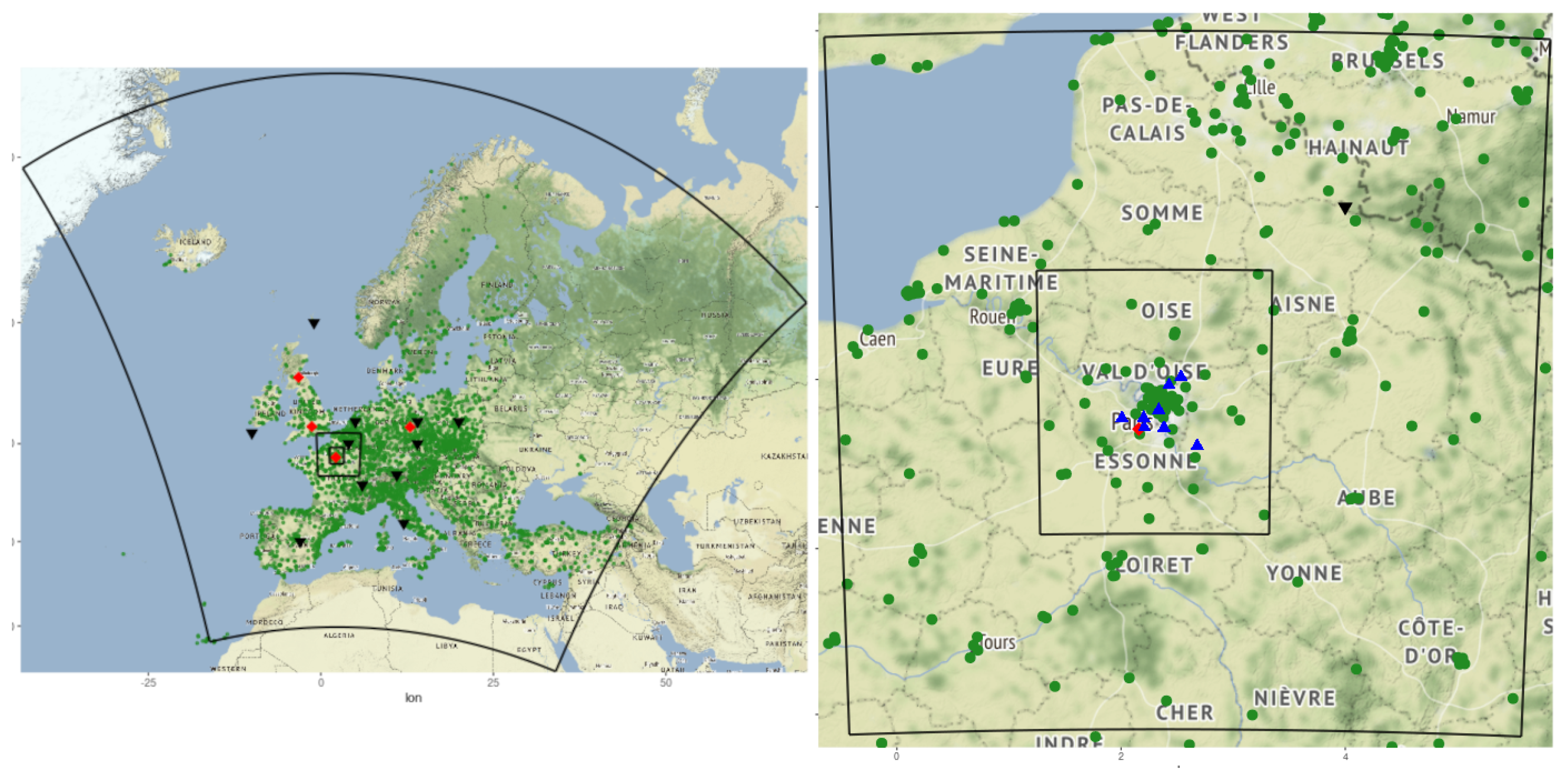
2.1. Observations

An exhaustive list of observations has been used for the validation of the reference simulation. For in situ surface measurements, we have used the EEA air quality control stations [24]. These stations are spread across Europe, covering multiple components including NO, NO${}_2$, O${}_3$ PM${}_{10}$ and PM${}_{2.5}$ as displayed in Figure 1. The number of stations with valid data differ per species (see Section 3). In this study, traffic stations have been discarded and only stations having more than 90% data availability for the simulation period have been used. Validation for vertical profiles of pressure, temperature and ozone using the data downloaded from the World Ozone and Ultraviolet Radiation Data Centre (WOUDC, [25]) resulting from Ozone Sonde measurements has been also included. Only 9 stations have data for the period of the simulations; February 2015; but the number of soundings per station are sufficient; therefore, the results will be included. More details will be given about these comparisons in Section 3.1.3. We have also integrated measurements from the EBAS database [26] for aerosol components, including ammonium, nitrates and organic aerosols.

Meteorological variables have also been added from several datasets. Two sources of data were used for meteorological variable measurements. The ECA&D project provides the E-OBS database [27], which contains measurements merged in an ensemble modelling procedure for the whole of Europe. This dataset includes daily values for temperature (average, minimum and maximum), average wind speed, relative humidity and precipitation. E-OBS is a gridded dataset resulting from an aggregation of observations over several years, gridded using a kriging procedure explained in the aforementioned reference. In our work, we have extracted (bilinear interpolation) the model outputs and E-OBS data at the location of EEA stations. The second dataset used is the British Atmospheric Data Centre network [28], providing hourly values for temperature, wind speed and precipitation. Meteorological data from Parisian measurement sites from the Météo-France (MF) network have also been integrated. These data are used for comparisons provided in Section 3.1.1.

2.2. WRF and CHIMERE

The CHIMERE CTM (chemistry-transport model) was first designed as a regional model for ozone simulations in the late 1990s [23,29]. It has since been developed more and more and has been used in different applications in both research and forecasts over several regions or continents ([30,31]). In its latest version (version 2020r3), it has been coupled with the Weather Research Forecast (WRF, v3.7.1) meteorological model, [32]. The coupled models can be used to quantify the retroactions of aerosols on meteorological variables via the direct and indirect effects. Global boundary/initial conditions for WRF are taken from NCEP-FNL 1${}^{\circ }$×1${}^{\circ }$ resolution global fields [33]. The CHIMERE model contains a wide range of gaseous atmospheric components as well as an aerosol module, taking into account BC (black carbon), sulfate, nitrate, ammonium, POA/SOA (primary/secondary organic aerosol), mineral dust, sea salt and PPM (primary particulate matter including organic aerosols). The model considers coagulation, nucleation and condensation processes, as well as wet and dry deposition. Aerosols are divided into 10 size bins via a sectional logarithmic scheme. Several types of anthropogenic and biogenic emissions encompassing biomass burning, mineral dust, sea salt, DMS, and nitrogen oxides from lightning are included in the model. More detailed descriptions of the model inputs and options used for this study are provided in Section 2.4 and Section 3.

The WRF and CHIMERE-v2020r3 models were run over a triple-nested domain, presented in Figure 1; the coarse domain (called FAIR30) covering the entire Europe with a 30 km × 30 km horizontal resolution, an intermediate domain (PAR10) with 10 km × 10 km resolution and the finest domain (PAR03) covering the Parisian area on a 3 km × 3 km horizontal resolution (3.33 km exactly to respect a 1/3 ratio between domain resolutions needed for WRF). Vertically and for CHIMERE, the simulation domain contains 15 layers, starting from the surface and ascending to 300 hPa. The first vertical level has a depth of 7 m. This vertical resolution remains unchanged for all domains. It should also be kept in mind that all simulations and emission reduction scenarios were conducted for all three domains in a coherent way over a target area defined as a rectangle defined by the range of longitude and latitude: 1.80${}^{\circ }$ E–2.90${}^{\circ }$ E and 48.30${}^{\circ }$ N–49.40${}^{\circ }$ N. For the WRF model, a gridded spectral nudging of the global meteorological variables (horizontal wind, potential temperature, geopotential height and the water vapor) is applied for the three domains within the Planetary Boundary Layer. A nudging factor of 0.0003 s${}^{-1}$ and a cutoff wavelength of 2500 km is used for all variables and domains. Vertically, the grid extends from the surface to 50 hPa and with 30 levels.

Figure 1. The simulations are run on a triple-nested configuration with a European domain with a 30 km resolution (FAIR30), an intermediary domain with a 10 km resolution (PAR10) and the finest domain focused on the Parisian region with roughly 3 km resolution (PAR03). Green circles are the EEA stations, red diamonds represent EBAS stations for NH${}_4^{+}$/NO${}_3^{-}$ measurements, black downward triangles show WOUDC OzoneSonde stations and blue triangles show météo-France stations used in this study. Ozone Sonde stations are not located in the two inner domains. Data were extracted from the E-OBS gridded fields by using the locations of EEA stations; therefore, stations for both are similar (green points).

Figure 1. The simulations are run on a triple-nested configuration with a European domain with a 30 km resolution (FAIR30), an intermediary domain with a 10 km resolution (PAR10) and the finest domain focused on the Parisian region with roughly 3 km resolution (PAR03). Green circles are the EEA stations, red diamonds represent EBAS stations for NH${}_4^{+}$/NO${}_3^{-}$ measurements, black downward triangles show WOUDC OzoneSonde stations and blue triangles show météo-France stations used in this study. Ozone Sonde stations are not located in the two inner domains. Data were extracted from the E-OBS gridded fields by using the locations of EEA stations; therefore, stations for both are similar (green points).

2.3. Anthropogenic Emissions

The anthropogenic emissions are taken from the CAMS regional emission inventory [34]. They provide a gridded distribution of anthropogenic emissions with a 0.1${}^{\circ }$× 0.05${}^{\circ }$ horizontal resolution over Europe. The emissions for the year 2015 are used in the anthropogenic emission pre-processor of CHIMERE, which regrids the data from the raw emission inventory onto the simulation domains. A set of emission input files for the base simulation were generated. Then, for each scenario, another set of emissions was generated with 25% and 50% reduction for selected PM precursor species (SO${}_x$, NH${}_3$, NMVOC and NO${}_x$), and primary PM${}_{10}$ (simply PPM here) and applied over all activity sectors.

2.4. Simulations and the Modeling Framework

The simulation period for the reference case is from the 1st to 28th of February 2015, chosen because of a major PM episode that occurred between 10th and 17th of February 2015. While the reference simulation was performed for the whole month to obtain a better picture of the magnitude of the episode and a more accurate validation, the emission reduction scenarios were only ran for the duration of the episode or for the episode plus some days before, as shown in

Table 1. Summary of simulations used in this study. All simulations mentioned in this table have been performed for all three domains, the “emission reduction domain” for the scenario part of the table regards to the domain from which the emission reductions have commenced.

Simulation	Reference
	Period			Coupling effect
Ref	01/02/2015–28/02/2015			No-coupling
Ref-CPL2	01/02/2015–28/02/2015			Direct effects
Ref-CPL3	01/02/2015–28/02/2015			Indirect effects
Ref-CPL4	01/02/2015–28/02/2015			Direct+indirect effects
Simulation	Scenario
	Period	Emission reduction	Emission reduction domain	Coupling effect
SO${}_x$	10/02/2015–17/02/2015	25%/50%	PAR03	No-coupling
NO${}_x$	10/02/2015–17/02/2015	25%/50%	PAR03	No-coupling
NMVOC	10/02/2015–17/02/2015	25%/50%	PAR03	No-coupling
PPM	10/02/2015–17/02/2015	25%/50%	PAR03	No-coupling
NH${}_3$	10/02/2015–17/02/2015	25%/50%	PAR03	No-coupling
ALL	10/02/2015–17/02/2015	25%/50%/100%	PAR03	No-coupling
CPL2-ALL	10/02/2015–17/02/2015	50%	PAR03	Direct effects
CPL3-ALL	10/02/2015–17/02/2015	50%	PAR03	Indirect effects
CPL4-ALL	10/02/2015–17/02/2015	50%	PAR03	Direct+indirect effects
ALL-redPAR10	10/02/2015–17/02/2015	50%	PAR10	No-coupling
ALL-redFAIR30	10/02/2015–17/02/2015	50%	FAIR30	No-coupling
ALL-2days	08/02/2015–17/02/2015	50%	PAR03	No-coupling
ALL-redPAR10-2days	08/02/2015–17/02/2015	50%	PAR10	No-coupling
ALL-redFAIR30-2days	08/02/2015–17/02/2015	50%	FAIR30	No-coupling
ALL-10days	01/02/2015– 17/02/2015	50%	PAR03	No-coupling
ALL-redPAR10-10days	01/02/2015–17/02/2015	50%	PAR10	No-coupling
ALL-redFAIR30-10days	01/02/2015–17/02/2015	50%	FAIR30	No-coupling

. Simulations were performed with or without direct/indirect aerosol effects on meteorological variables. In total, 28 simulations are performed.

• Ref: A reference simulation corresponding to the offline mode. This simulation is used as the reference case that the scenarios are compared to.
• Ref-CPL2, Ref-CPL3 and Ref-CPL4: Same as Ref but with the coupling effects. These simulations are to be compared to both the offline reference simulation as well as the coupled scenarios mentioned below.
• 2 × 6 simulations with a 25% and 50% decrease in anthropogenic emissions and using the offline configuration of Ref. These scenarios aim to analyze the effect of the different degrees of emission reductions for a list of species compared to the reference simulation (named Ref above).
• One simulation reducing all emissions by 100% for the fine domain. This simulation is performed to assess the background and transported concentrations.
• Three additional simulations, CPL2-ALL, CPL3-ALL and CPL4-ALL, mixing the effects of the WRF-CHIMERE coupling and the 50% of anthropogenic emissions. These scenarios are performed to assess the aerosol effects on meteorological fields and emission reductions.
• Two simulations applying a 50% decrease to the emissions of all aforementioned groups on the intermediate domain (ALL-redPAR10) and on the continental domain (ALL-redFAIR30). These scenarios aim to assess the changes observed in concentrations when emissions are reduced on a larger domain compared to the scenarios mentioned above.
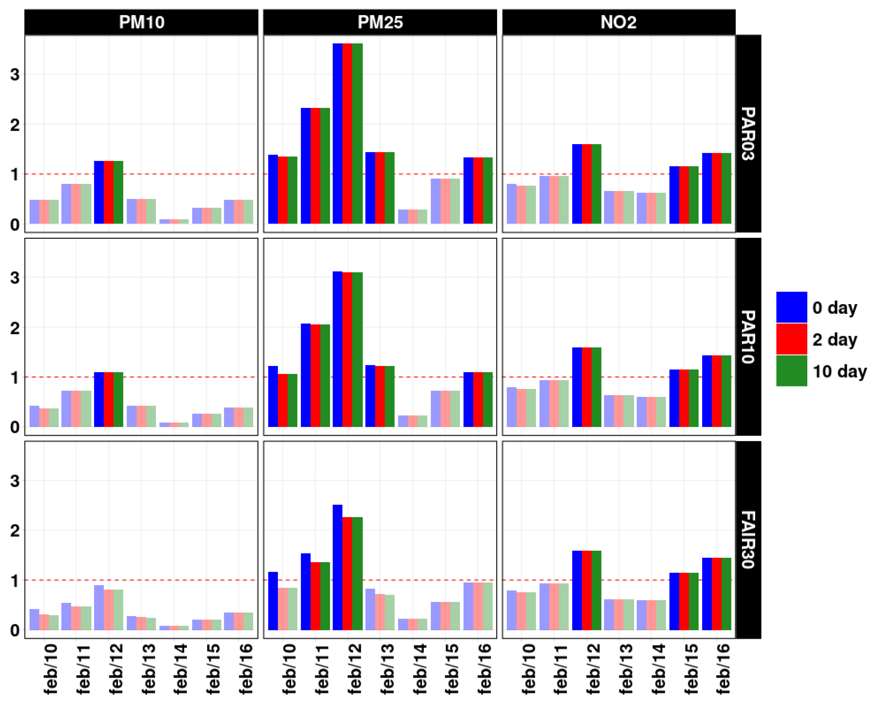
• Six simulations applying a 50% reduction decrease to the emissions of each of the three domains starting several days before the episode the start, i.e., the 8th and the the 1st. These scenarios are performed to understand the effect of the emission reduction starting time on the concentrations of pollutants observed during the episode.

For the boundary/initial conditions, the CAMS global 3-hourly reanalysis simulations [35] have been used. For both horizontal and vertical advection schemes, the VanLeer scheme [36] is used. The MELCHIOR2 [37] chemistry mechanism has been used in these simulations for the gaseous phase. The aerosol species are distributed into 10 bins, starting from 10 nm and going up to 40 $\mathsf{\mu }$m. A simple 2-product scheme was used for the simulation of SOA ([38,39]). The partitioning of inorganic species between gaseous/aerosol phases is handled by the ISORROPIA module [40] which has been coupled internally with the model. The fastJ model [41] has also been included within CHIMERE providing parameters regarding radiation and photolysis [42]. Biogenic emissions are simulated by the MEGANv2.1 [43] model, internally coupled to the model. Sea salt emissions have been calculated using the Monahan scheme [44]. Lightning NO${}_x$ emissions have also been included using the scheme explained in [23]. Mineral dust emissions are estimated by a threshold process presented by [45] with the addition of some improvements (see [46] for more details). DMS (Dimethyl Sulfide) emissions are also included using the [47] scheme; more details provided in the model description article [46]. For landcover data, the GLOBCOVER database has been used [48]. Fire emissions are not included. There were no significant fires during the simulation period that would affect the simulation domain. None of the aforementioned parameters change between the reference simulation and the emission reduction scenarios.

3. The Reference Simulation

In this section, a validation of the reference simulation is presented using observations mentioned in Section 2.1. An analysis of the PM component of this simulation is presented. Finally, a comparison is performed between the simulations including direct/indirect aerosol effects and the corresponding reference cases. The location of stations are shown in Figure 1. The statistics and the figures presented in the following section were produced with Evaltools, a python package providing different tools for model/observation comparisons. The metrics provided in Table 2 and Table 3 are explained in the documentation of the Evaltools package [49]. More information about how these metrics are calculated can be observed in [50].

3.1. Evaluation of the Reference Simulation

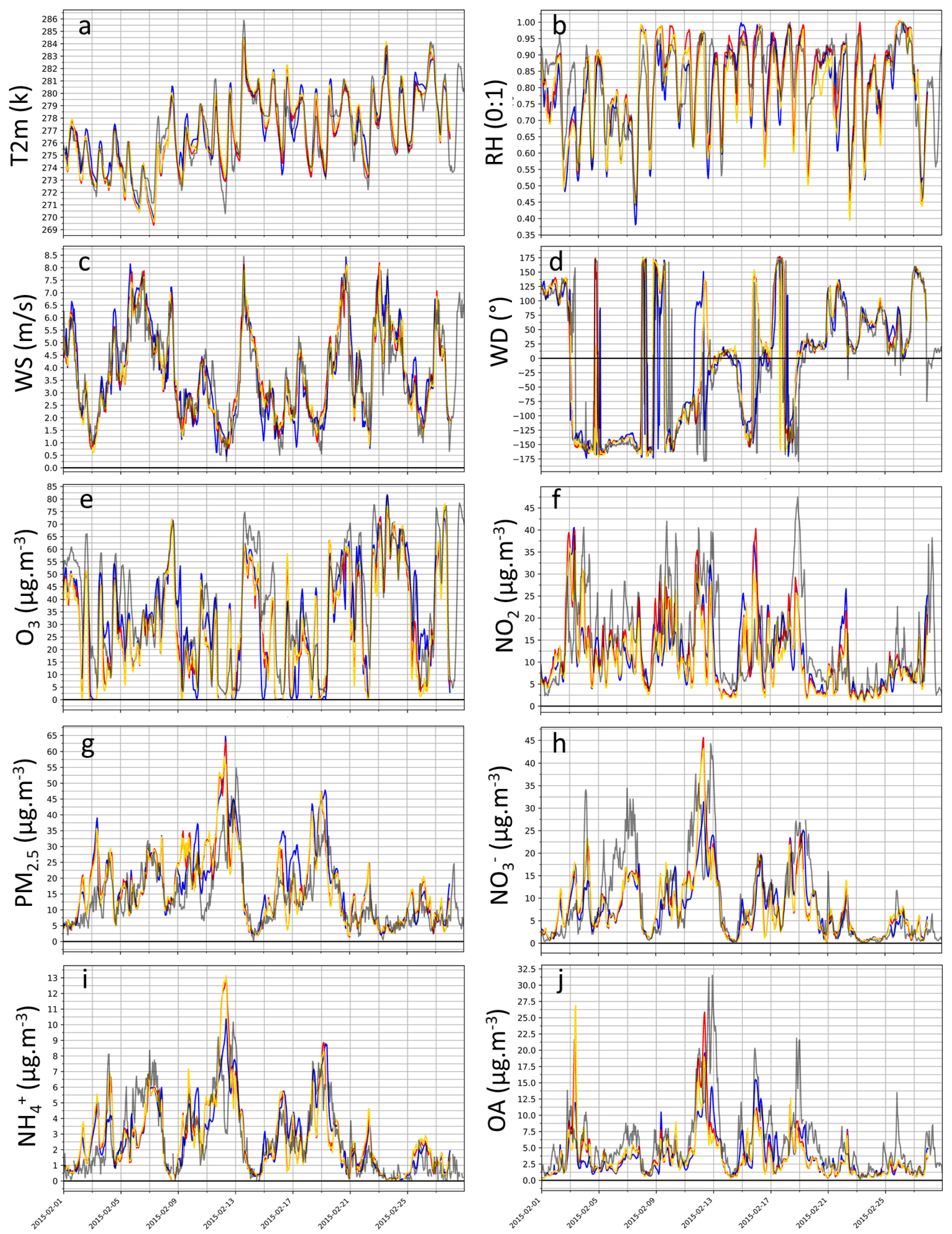
3.1.1. Meteorological Variables

Table 2 shows the error statistics for daily minimum, maximum and average temperature, average wind speed, precipitation and relative humidity with the E-OBS dataset. For the three domains, the model reproduced the evolution of the temperature (maximum and average values) well; however, an underestimation of the daily minimum value is observed. Wind speed is also well represented in the two coarser domains; however, in the finest domain only one station with a complete set of data was found (not presented here because of the statistic sample being too small). Relative humidity is also well reproduced by the model. It should be mentioned that the representation of common stations between the three domains is quite similar, meaning that a higher resolution does not automatically mean better representation of meteorological conditions, at least for this period of the year and for this region.

Meteorological data from Météo-France and those from the SIRTA observatory [51] were also added. In total, eight stations in the Parisian area were used for these comparisons (Figure 1). The representation of these four meteorological variables is quite correctly conducted by the model for all three domains similar to the E-OBS dataset. These comparisons show (Figure 2, (a):(d)) that the resolution seems not to be a key issue for the accuracy of the meteorological variables. In all cases, the correlation is slightly improved when the resolution increases. Since a spectral nudging is activated, the weak differences between the domains is expected since the nested domains remain influenced by the large scale patterns, which include observations. Nudging is efficient to avoid divergences of meteorological simulations; however, at a local scale an improvement is expected with much more detailed processes influencing the simulation.

Figure 2. Time series for meteorological variables and surface concentrations. Data are averaged for all stations included in the PAR03 domain and for each corresponding cell of the modeled domains (PAR03, PAR10 and FAIR30). The name and the unit for each variable/species is written on the left side of each plot. Simulations for FAIR30 are shown in blue, PAR10 in red and PAR03 in gold. Statistics for these species/variables are shown in Table 2 and Table 3. Panels (a–d) show temperature (T2M), relative humidity (RH), wind speed (WS) and wind direction (WD) respectively. Panels (e,f) show ozone (O₃) and nitrogen dioxide (NO₂) while panels (g–j) show PM_2.5, nitrates (${\mathrm{NO}}_3^{-}$), ammonium (${\mathrm{NH}}_4^{+}$) and organic aerosols (OA) respectively.

Figure 2. Time series for meteorological variables and surface concentrations. Data are averaged for all stations included in the PAR03 domain and for each corresponding cell of the modeled domains (PAR03, PAR10 and FAIR30). The name and the unit for each variable/species is written on the left side of each plot. Simulations for FAIR30 are shown in blue, PAR10 in red and PAR03 in gold. Statistics for these species/variables are shown in Table 2 and Table 3. Panels (a–d) show temperature (T2M), relative humidity (RH), wind speed (WS) and wind direction (WD) respectively. Panels (e,f) show ozone (O₃) and nitrogen dioxide (NO₂) while panels (g–j) show PM_2.5, nitrates (${\mathrm{NO}}_3^{-}$), ammonium (${\mathrm{NH}}_4^{+}$) and organic aerosols (OA) respectively.

Table 2. Error statistic for meteorological parameters shown in Figure 3. Units are given on the left side of each section. Comparisons are separated by type of station, and types of stations are also given on the left side of each section. All the stations are shown in (Figure 2). The values given in the brackets for FAIR30 and PAR10 show the error statistics for common stations between all domains.

Variable	Domain	Model Mean	Obs Mean	RMSE	MeanBias	PearsonR (−1:1)	No. Stations
Tmax (K) (E-OBS)	FAIR30	278.02 (279.58)	279.52 (280.10)	2.34 (1.33)	−1.51 (−0.53)	0.85 (0.90)	3571
	PAR10	278.97 (279.60)	279.66 (280.10)	1.38 (1.13)	−0.69 (−0.50)	0.89 (0.93)	270
	PAR03	279.76	280.11	1.06	−0.35	0.93	56
Tmean (K) (E-OBS)	FAIR30	274.74 (276.63)	275.88 (277.11)	1.85 (1.03)	−1.15 (−0.48)	0.89 (0.93)	3571
	PAR10	275.88 (276.65)	276.59 (277.11)	1.29 (0.95)	−0.71 (−0.46)	0.90 (0.94)	270
	PAR03	276.75	277.12	0.96	−0.37	0.94	56
Tmin (K) (E-OBS)	FAIR30	271.77 (273.89)	272.58 (274.09)	2.35 (1.42)	−0.81 (−0.20)	0.80 (0.83)	3571
	PAR10	272.88 (273.97)	273.78 (274.09)	1.91 (1.29)	−0.90 (−0.12)	0.80 (0.87)	270
	PAR03	274.05	274.10	1.36	−0.05	0.85	56
T (K) (MF)	FAIR30	276.87	276.91	0.90	−0.04	0.94	8
	PAR10	276.71	276.91	0.82	−0.20	0.95	8
	PAR03	276.94	276.91	0.88	0.03	0.95	8
T (K) (WOUDC)	FAIR30	264.58 (266.19)	263.11 (264.91)	6.15 (4.96)	1.62 (1.32)	0.995 (0.997)	11
	PAR10	265.49	263.98	5.42	1.50	0.998	1
	PAR03	–	–	–	–	–	–
WSmean (m/s) (E-OBS)	FAIR30	6.12	4.36	2.60	1.76	0.80	533
	PAR10	4.34	3.86	0.99	0.49	0.91	13
	PAR03	–	–	–	–	–	–
WS (m/s) (MF)	FAIR30	3.84	3.77	0.95	0.08	0.89	8
	PAR10	3.77	3.77	1.00	0.01	0.90	8
	PAR03	3.75	3.77	1.00	−0.01	0.90	8
RHmean (0:1) (E-OBS)	FAIR30	0.87 (0.81)	0.82 (0.83)	0.10 (0.05)	0.05 (−0.01)	0.64 (0.81)	533
	PAR10	0.85 (0.81)	0.83 (0.83)	0.07 (0.06)	0.02 (−0.01)	0.71 (0.80)	18
	PAR03	0.80	0.83	0.07	−0.03	0.79	7
RH (0:1) (MF)	FAIR30	0.80	0.82	0.06	−0.02	0.81	8
	PAR10	0.82	0.82	0.05	−0.00	0.81	8
	PAR03	0.80	0.82	0.06	−0.02	0.80	8

Table 2. Error statistic for meteorological parameters shown in Figure 3. Units are given on the left side of each section. Comparisons are separated by type of station, and types of stations are also given on the left side of each section. All the stations are shown in (Figure 2). The values given in the brackets for FAIR30 and PAR10 show the error statistics for common stations between all domains.

Variable	Domain	Model Mean	Obs Mean	RMSE	MeanBias	PearsonR (−1:1)	No. Stations
Tmax (K) (E-OBS)	FAIR30	278.02 (279.58)	279.52 (280.10)	2.34 (1.33)	−1.51 (−0.53)	0.85 (0.90)	3571
	PAR10	278.97 (279.60)	279.66 (280.10)	1.38 (1.13)	−0.69 (−0.50)	0.89 (0.93)	270
	PAR03	279.76	280.11	1.06	−0.35	0.93	56
Tmean (K) (E-OBS)	FAIR30	274.74 (276.63)	275.88 (277.11)	1.85 (1.03)	−1.15 (−0.48)	0.89 (0.93)	3571
	PAR10	275.88 (276.65)	276.59 (277.11)	1.29 (0.95)	−0.71 (−0.46)	0.90 (0.94)	270
	PAR03	276.75	277.12	0.96	−0.37	0.94	56
Tmin (K) (E-OBS)	FAIR30	271.77 (273.89)	272.58 (274.09)	2.35 (1.42)	−0.81 (−0.20)	0.80 (0.83)	3571
	PAR10	272.88 (273.97)	273.78 (274.09)	1.91 (1.29)	−0.90 (−0.12)	0.80 (0.87)	270
	PAR03	274.05	274.10	1.36	−0.05	0.85	56
T (K) (MF)	FAIR30	276.87	276.91	0.90	−0.04	0.94	8
	PAR10	276.71	276.91	0.82	−0.20	0.95	8
	PAR03	276.94	276.91	0.88	0.03	0.95	8
T (K) (WOUDC)	FAIR30	264.58 (266.19)	263.11 (264.91)	6.15 (4.96)	1.62 (1.32)	0.995 (0.997)	11
	PAR10	265.49	263.98	5.42	1.50	0.998	1
	PAR03	–	–	–	–	–	–
WSmean (m/s) (E-OBS)	FAIR30	6.12	4.36	2.60	1.76	0.80	533
	PAR10	4.34	3.86	0.99	0.49	0.91	13
	PAR03	–	–	–	–	–	–
WS (m/s) (MF)	FAIR30	3.84	3.77	0.95	0.08	0.89	8
	PAR10	3.77	3.77	1.00	0.01	0.90	8
	PAR03	3.75	3.77	1.00	−0.01	0.90	8
RHmean (0:1) (E-OBS)	FAIR30	0.87 (0.81)	0.82 (0.83)	0.10 (0.05)	0.05 (−0.01)	0.64 (0.81)	533
	PAR10	0.85 (0.81)	0.83 (0.83)	0.07 (0.06)	0.02 (−0.01)	0.71 (0.80)	18
	PAR03	0.80	0.83	0.07	−0.03	0.79	7
RH (0:1) (MF)	FAIR30	0.80	0.82	0.06	−0.02	0.81	8
	PAR10	0.82	0.82	0.05	−0.00	0.81	8
	PAR03	0.80	0.82	0.06	−0.02	0.80	8

Table 3. Error statistic for chemical species shown in Figure 3. Units are given on the left side of each section. Comparisons are separated by type of station; types of stations are also given on the left side of each section. All the stations are shown in (Figure 2). The values given in the brackets for FAIR30 and PAR10 show the error statistics for common stations between all domains.

Species	Domain	Model Mean ($\mathsf{\mu }$g·m${}^{-3}$)	Obs Mean ($\mathsf{\mu }$g·m${}^{-3}$)	RMSE ($\mathsf{\mu }$g·m${}^{-3}$)	MeanBias ($\mathsf{\mu }$g·m${}^{-3}$)	PearsonR (−1:1)	No. Stations
O${}_{\mathbf{3}}$ (EEA)	FAIR30	47.70 (35.87)	45.35 (37.99)	15.67 (10.15)	2.35 (−2.12)	0.63 (0.85)	3571
	PAR10	38.29 (35.53)	40.13 (37.99)	9.17 (9.60)	−1.84 (−4.46)	0.87 (0.88)	270
	PAR03	33.03	37.99	9.87	−4.96	0.89	56
O${}_{\mathbf{3}}$ (WOUDC)	FAIR30	45.32 (43.60)	40.62 (39.72)	18.86 (10.94)	4.70 (3.88)	0.85 (0.93)	11
	PAR10	47.67	40.90	12.84	6.77	0.90	1
	PAR03	–	–	–	–	–	–
NO${}_{\mathbf{2}}$ (EEA)	FAIR30	9.98 (20.68)	24.47 (35.81)	16.82 (17.23)	−14.49 (−15.13)	0.54 (0.72)	3571
	PAR10	18.72 (30.35)	27.34 (35.81)	11.88 (11.20)	−8.63 (−5.46)	0.74 (0.74)	270
	PAR03	32.80	35.81	11.22	−3.02	0.74	56
PM${}_{\mathbf{10}}$ (EEA)	FAIR30	20.31 (20.36)	26.20 (23.83)	14.42 (7.25)	−5.89 (−3.46)	0.66 (0.82)	3571
	PAR10	22.19 (22.04)	22.91 (23.83)	8.44 (7.85)	−0.72 (−1.79)	0.82 (0.84)	270
	PAR03	22.43	23.83	8.11	−1.40	0.82	56
PM${}_{\mathbf{2}.\mathbf{5}}$ (EEA)	FAIR30	18.87 (18.53)	19.13 (16.47)	10.67 (5.48)	−0.26 (2.06)	0.77 (0.90)	3571
	PAR10	21.43 (19.65)	17.12 (16.47)	8.92 (7.14)	4.31 (3.18)	0.82 (0.85)	270
	PAR03	19.93	16.47	7.51	3.45	0.86	56
NH${}_{\mathbf{4}}^{+}$ (EBAS)	FAIR30	2.34 (2.65)	2.49 (2.56)	2.34 (1.36)	−0.15 (0.10)	0.38 (0.82)	4
	PAR10	2.74	2.56	1.70	0.18	0.74	1
	PAR03	2.75	2.56	1.73	0.19	0.74	1
NO${}_{\mathbf{3}}^{-}$ (EBAS)	FAIR30	6.48 (7.55)	6.57 (9.44)	6.52 (6.18)	−0.09 (−1.89)	0.39 (0.38)	4
	PAR10	7.99	9.44	6.69	−1.45	0.79	1
	PAR03	7.95	9.44	6.80	−1.48	0.79	1
OA (EBAS)	FAIR30	3.43 (3.44)	4.58 (5.61)	1.94 (3.95)	−1.16 (−2.16)	0.94 (0.76)	6
	PAR10	3.61	5.61	4.29	−2.00	0.66	1
	PAR03	3.36	5.61	4.51	−2.24	0.63	1

Table 3. Error statistic for chemical species shown in Figure 3. Units are given on the left side of each section. Comparisons are separated by type of station; types of stations are also given on the left side of each section. All the stations are shown in (Figure 2). The values given in the brackets for FAIR30 and PAR10 show the error statistics for common stations between all domains.

Species	Domain	Model Mean ($\mathsf{\mu }$g·m${}^{-3}$)	Obs Mean ($\mathsf{\mu }$g·m${}^{-3}$)	RMSE ($\mathsf{\mu }$g·m${}^{-3}$)	MeanBias ($\mathsf{\mu }$g·m${}^{-3}$)	PearsonR (−1:1)	No. Stations
O${}_{\mathbf{3}}$ (EEA)	FAIR30	47.70 (35.87)	45.35 (37.99)	15.67 (10.15)	2.35 (−2.12)	0.63 (0.85)	3571
	PAR10	38.29 (35.53)	40.13 (37.99)	9.17 (9.60)	−1.84 (−4.46)	0.87 (0.88)	270
	PAR03	33.03	37.99	9.87	−4.96	0.89	56
O${}_{\mathbf{3}}$ (WOUDC)	FAIR30	45.32 (43.60)	40.62 (39.72)	18.86 (10.94)	4.70 (3.88)	0.85 (0.93)	11
	PAR10	47.67	40.90	12.84	6.77	0.90	1
	PAR03	–	–	–	–	–	–
NO${}_{\mathbf{2}}$ (EEA)	FAIR30	9.98 (20.68)	24.47 (35.81)	16.82 (17.23)	−14.49 (−15.13)	0.54 (0.72)	3571
	PAR10	18.72 (30.35)	27.34 (35.81)	11.88 (11.20)	−8.63 (−5.46)	0.74 (0.74)	270
	PAR03	32.80	35.81	11.22	−3.02	0.74	56
PM${}_{\mathbf{10}}$ (EEA)	FAIR30	20.31 (20.36)	26.20 (23.83)	14.42 (7.25)	−5.89 (−3.46)	0.66 (0.82)	3571
	PAR10	22.19 (22.04)	22.91 (23.83)	8.44 (7.85)	−0.72 (−1.79)	0.82 (0.84)	270
	PAR03	22.43	23.83	8.11	−1.40	0.82	56
PM${}_{\mathbf{2}.\mathbf{5}}$ (EEA)	FAIR30	18.87 (18.53)	19.13 (16.47)	10.67 (5.48)	−0.26 (2.06)	0.77 (0.90)	3571
	PAR10	21.43 (19.65)	17.12 (16.47)	8.92 (7.14)	4.31 (3.18)	0.82 (0.85)	270
	PAR03	19.93	16.47	7.51	3.45	0.86	56
NH${}_{\mathbf{4}}^{+}$ (EBAS)	FAIR30	2.34 (2.65)	2.49 (2.56)	2.34 (1.36)	−0.15 (0.10)	0.38 (0.82)	4
	PAR10	2.74	2.56	1.70	0.18	0.74	1
	PAR03	2.75	2.56	1.73	0.19	0.74	1
NO${}_{\mathbf{3}}^{-}$ (EBAS)	FAIR30	6.48 (7.55)	6.57 (9.44)	6.52 (6.18)	−0.09 (−1.89)	0.39 (0.38)	4
	PAR10	7.99	9.44	6.69	−1.45	0.79	1
	PAR03	7.95	9.44	6.80	−1.48	0.79	1
OA (EBAS)	FAIR30	3.43 (3.44)	4.58 (5.61)	1.94 (3.95)	−1.16 (−2.16)	0.94 (0.76)	6
	PAR10	3.61	5.61	4.29	−2.00	0.66	1
	PAR03	3.36	5.61	4.51	−2.24	0.63	1

Figure 3. PM composition in the reference simulation as time series (left) and the average pie charts (right) showing three domains (each row one domain) in $\mathsf{\mu }$g·m${}^{-3}$. The plots are calculated using the average of stations common for all three domains.

Figure 3. PM composition in the reference simulation as time series (left) and the average pie charts (right) showing three domains (each row one domain) in $\mathsf{\mu }$g·m${}^{-3}$. The plots are calculated using the average of stations common for all three domains.

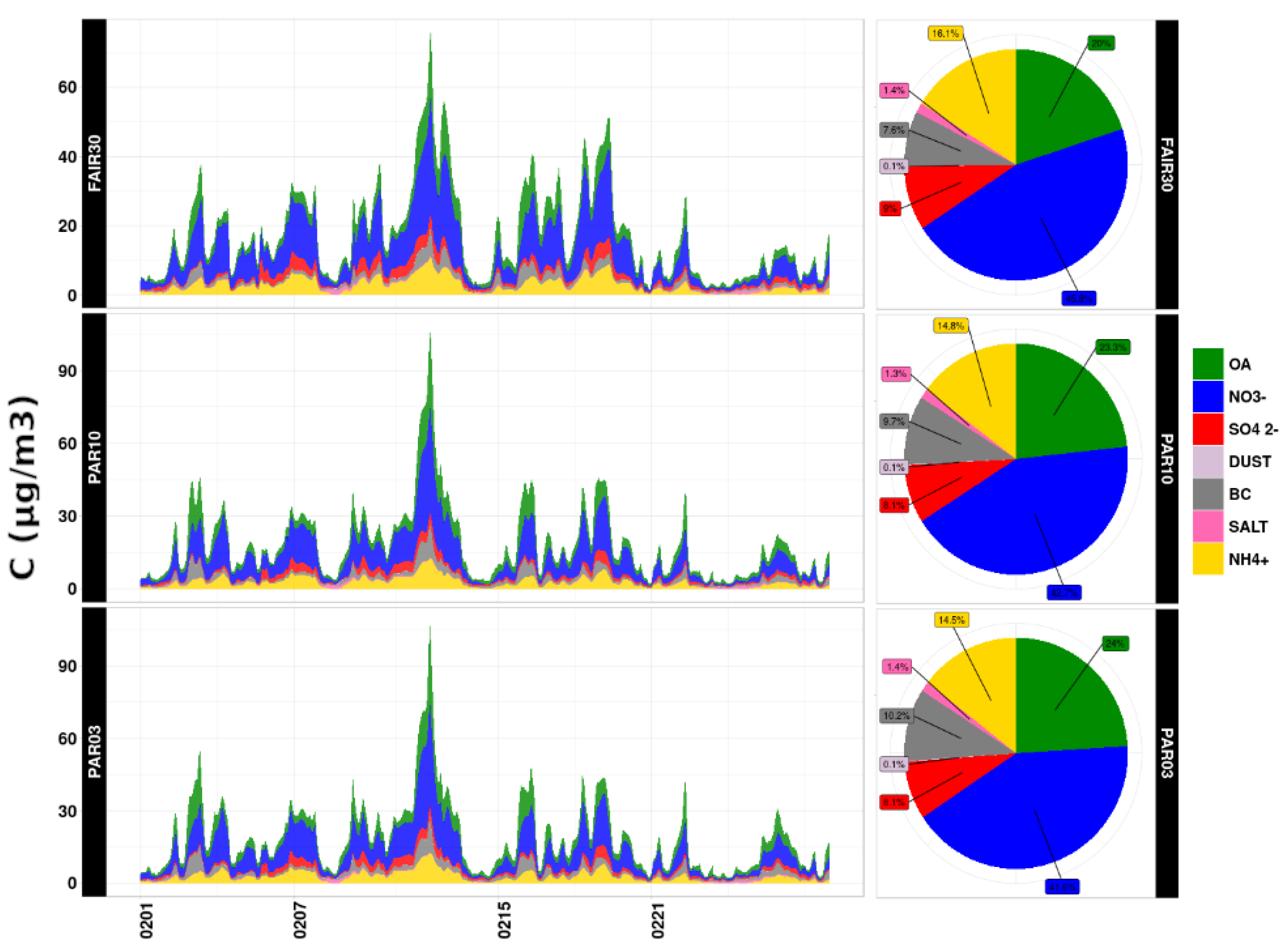
3.1.2. Surface Concentrations

Criteria Pollutants

Simulated concentrations of O${}_3$, NO${}_2$, PM${}_{10}$ and PM${}_{2.5}$ were compared to the EEA air quality stations. The time series for the four aforementioned species averaged over all available stations for each domain are shown in Figure 2, while the error statistics for these time series for each domain are shown in Table 3.

O${}_3$ daily maxima are underestimated, while the daily minima seem to be reproduced accurately. This underestimation in daily peaks explains the negative bias reported in Table 3. However, the overall trend of O${}_3$ is well represented. The same behavior is observed for NO${}_2$, an overall correct simulation of the profile, while the maxima are underestimated. For the particulate matter comparisons, the time evolution is quite well reproduced, while some of the peaks seem to be overestimated. Regarding the PM episode observed in measurements, the model successfully simulates this episode both in time evolution and magnitude.

It is interesting to note that in the case of these four species, the finest domain shows better performances compared to the other two coarser domains regarding to all the statistical metrics provided. However, it can be argued that the number of stations for the finer domain is less than the coarse domain; therefore, the statistical sample is not large enough to obtain a robust statement. To counter this issue, the comparisons were repeated for the common stations in the three domains. Comparing the common stations in all three domains presents a similar conclusion for O${}_3$ and NO${}_2$, albeit the results being closer to the third domain. This is probably because anthropogenic emissions are better spatially distributed in a finer domain, both, therefore, the concentration of NO${}_2$ and the production and transport of O${}_3$ are better simulated. Literature on this subject is quite abundant; ref. [52] examined the effect of horizontal resolution on the simulation of ozone, and ref. [53] examined the effect of increase in horizontal resolution on the representativeness of simulated ozone concentrations in comparison with the in situ measurement. Moreover, ref. [54] examined the same effect on an ensemble of models over Europe and more recently, ref. [55] examined the sensitivity to the horizontal resolution on an urban canopy on air quality simulations. For PM${}_{10}$ and PM${}_{2.5}$ this is not the case, and the results seem to be similarly represented in all three domains when looking at common stations. This is because of the higher homogeneity of the PM species spatially compared to O${}_3$ and NO${}_2$, PM also being influenced by long range transport.

PM Components

In addition, nitrate (NO${}_3^{-}$), ammonium (NH${}_4^{+}$) and total organic aerosols (OA) were compared to data obtained from the EBAS database presented in Figure 2h–j. Sulfates (SO${}_4^{2-}$) and black carbon (BC) are not presented since no complete and reliable data were found for any of the domains for these species. It should also be noted that only stations having hourly data were used for these comparisons; stations having daily data were filtered out. In the end, four and one stations were used for the coarse and the intermediate domain, respectively. The results demonstrate a good correlation between the measurements and the observations; the episode is simulated at the right time by the model and the intensity of the simulation matches the observations as well, especially for the coarse domain. This is true for NO${}_3^{-}$, NH${}_4^{+}$ and OA. Only one station is available for all three components for the two finer domains; while the correlation for these species remains quite high for the finer domains, there seems to be a stronger bias for NO${}_3^{-}$. The bias remains similar to the coarse domain for NH${}_4^{+}$ and OA. While the model manages to perfectly simulate the episode, another smaller peak is observed between the 5th and the 9th for NO${}_3^{-}$ in the observations: the model can observe the episode; however, it underestimates its intensity. A similar issue for the same peak is noted for OA, where the model captures the episode. The simulations are in February, and the SOA formation is limited to the anthropogenic part of it, since it is still too early in the year for biogenic SOA formation to occur. The part of the OA that is observed in these simulations contains only freshly emitted POA and anthropogenic SOA to a lower degree.

Since the model simulates total PM${}_{2.5}$ as well as NO${}_3^{-}$, NH${}_4^{+}$ and OA in a satisfactory manner, the distribution of PM components will be analyzed here as well. While the total PM${}_{10}$ is also well simulated, it is more difficult to make assumptions about the distribution of PM${}_{10}$ components, since larger particles such as dust and sea salt have to be considered as well. The major contribution of the PM${}_{2.5}$ concentration comes from NO${}_3^{-}$ for the Parisian region over the entire period of the simulations (Figure 3) followed by OA (containing mainly fresh emitted OC) and NH${}_4^{+}$. The distribution of PM${}_{2.5}$ components shows differences through the three domains, but the averaged distribution is similar. The main cause of concentration differences between the three domains seems to be from the lower simulated concentration of OA. For PM${}_{10}$, the three major contributors for the Parisian region remain the same as PM${}_{2.5}$. The contribution of salt remains low, around 1.4%, and mineral dust mainly issued from the Sahara is negligible during this episode.

3.1.3. Ozone Vertical Profile

The evaluation with ozone sondes data described in Section 2.1 is presented here. These data aim to validate the vertical simulation of pressure, temperature and ozone concentrations. The number of available stations for these comparisons are limited; in fact, there are no stations in the finest domain with usable data for our simulation period. Therefore, only the performance of the model for the coarse FAIR30 and the intermediate PAR10 domains are presented here. There are 11 stations with available data for the simulation period on the coarse domain, and only one station has a consistent dataset for the intermediate domain (Figure 1).

The results of these comparisons are shown in Figure 4, which displays an averaged profile for the 11 stations on the coarse domain and the one station on the intermediate domain. Overall statistics are presented in Table 2 and Table 3 for the temperature and O${}_3$, respectively. The temperature is well represented in the model; however, in the last levels of the model, a bias is observed. This is not much of a concern for our comparisons, since these altitudes are not going to affect surface-level simulations. When looking at ozone comparisons, the same issue is visible. While the simulated concentrations fit quite well to the first 12 levels of the model, a bias is observed for the last three levels. The last levels are very sensitive to the top boundary conditions that have been used; this bias is the signature of biased boundary conditions from the CAMS reanalysis at the top of the domain. It could also be an issue with the mass fluxes at the top of the model.

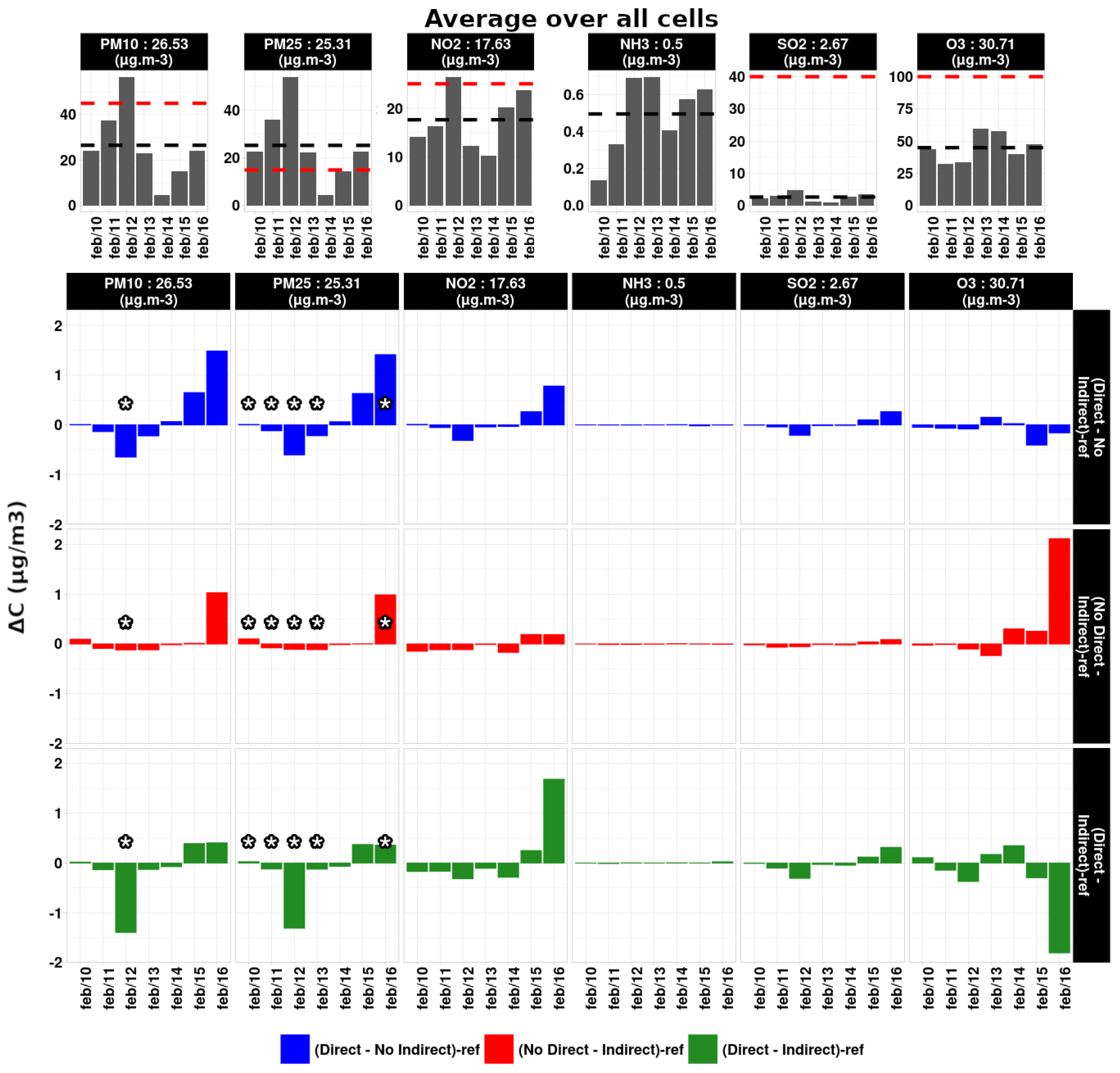
3.2. Effect of Chemistry-Meteorology Couplings

The online coupling between WRF and CHIMERE has been implemented in order to take into account the direct/indirect effects of aerosols on meteorological variables ([56,57]). The CHIMERE model offers the possibility to switch-on/off the coupling and allows for various configurations. When the coupling between WRF and CHIMERE is activated, it enables us to include the direct and indirect effects of aerosols on meteorological conditions, making the simulation more realistic by replacing the default WRF chemical climatologies. In our case, the coupling seems to have weak effects on the comparison of the simulations versus observations both at the surface and along vertical profiles (not shown here). There is a slight increase in correlations and a slight decrease in biases observed for all compared species, but they do not seem to be significant. When looking at meteorological variables, the same behavior is observed. The results being quite similar to what is shown in the previous sections (both for meteorological variables and chemical species) for the offline simulations, the validation for the coupling case has not been shown here. The effects of the coupling will also be studied with the emission reduction scenarios.

4. Emission Reduction Scenarios

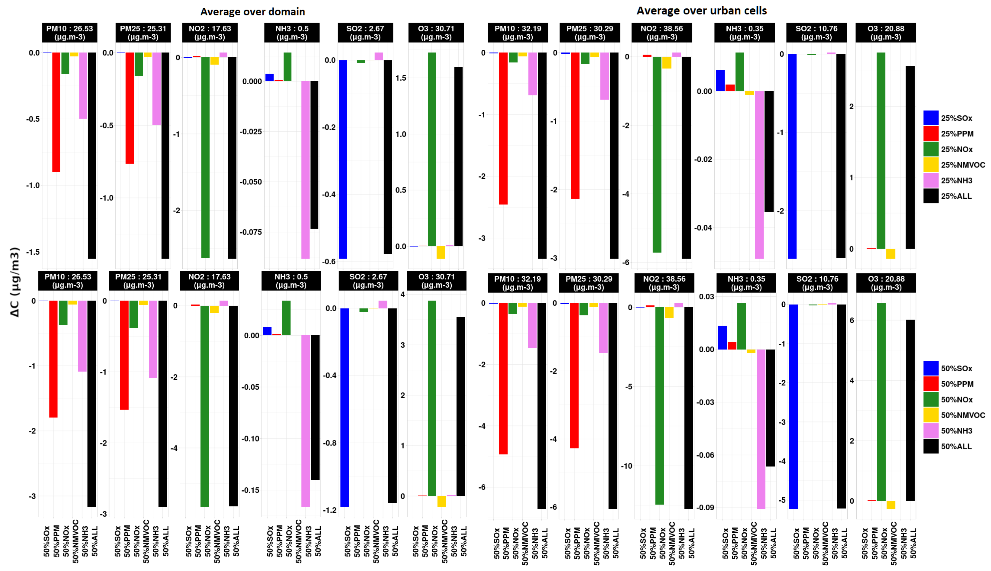
4.1. Analysis of Scenarios over the Fine Domain

The average changes over the episode period for the finest domain are discussed here. Figure 5 shows the deltas defined as the difference between a scenario and the base case. For a selected number of species, this delta is provided for the 25% and 50% reduction scenarios averaged over the entire domain. The value given on top of each plot shows the average of the reference simulation. Depending on the species, an emission reduction causes a negative or a positive delta. The differences are mentioned in percentage change in the text while delta concentration is shown in the figures, making both available.

For example, in all scenarios, both for 25% and 50% reductions, a concentration decrease of PM${}_{10}$ and PM${}_{2.5}$ is observed, resulting in a maximum reduction of −6.0%/−5.6% and −12.0%/−11.8% for PM${}_{10}$/PM${}_{2.5}$ for 25%ALL and 50%ALL scenarios, respectively, for urban cells. As expected, the scenario that causes maximum changes to PM${}_{10}$/PM${}_{2.5}$ concentrations is the 25%ALL/50%ALL one. This is due to a simultaneous decrease in NO${}_3^{-}$, OA, NH${}_4^{+}$ and BC concentrations. For stations located in the Parisian area, a 50% reduction in all emissions corresponds to −10.0%, −28.0%, −8.2% and −36.1% reduction in concentrations of NO${}_3^{-}$, OA, NH${}_4^{+}$ and BC, respectively, while the rest of the species either shows negligible concentrations to begin with (case of Dust and Salt) or shows negligible change in concentration (case of SO${}_4^{2-}$). Of course, looking at specific scenarios other than the 25%ALL/50%ALL means that the concentrations of these species do not change at the same time anymore. The 25%PPM/50%PPM scenarios cause the same reduction as reductions to 25%ALL/50%ALL scenarios on OA and BC concentrations, while 25%NO${}_x$/50%NO${}_x$ induce same changes as 25%ALL/50%ALL scenarios only to NO${}_3^{-}$ and NH${}_4^{+}$. The scenario that triggers the least reduction in PM concentrations is the SO${}_x$ emission reduction scenario; this might be because the concentration of SO${}_4^{2-}$ in both PM${}_{2.5}$ and PM${}_{10}$ is much lower than the major components contributing to PM${}_{2.5}$ concentration such as NO${}_3^{-}$ and OA. The SO${}_x$ emission reduction scenarios do not cause any changes to SO${}_4^{2-}$ concentrations, much like the 25%ALL/50%ALL scenarios. It is noteworthy that a −50% emission reduction of NH${}_3$ is more efficient to reduce PM than a reduction of a −50% emission reduction of NO${}_x$, while the absolute total amount of the reduced NH${}_3$ emission is about 10 times less than the one of NO${}_x$. Two main reasons to explain this feature: (i) the molar mass ratio between NO${}_3^{-}$ and NH${}_4^{+}$ is 3.5 leading to an intrinsic more efficient reduction of PM through ammonia emission reductions, (ii) total ammonium concentrations are usually in default over urban areas, enhancing the efficiency of ammonia emission reductions (Nitrate-limited regime). By reducing NO${}_x$ emissions, we could have expected an increase in ammonia concentrations, since less ammonium nitrate will be produced. However, as the dry deposition velocity of PM is by far less important than NH${}_3$ deposition velocity, there is then a competition process hampering the increase in ammonia concentration. The ammonium nitrate formation can be observe as a process increasing the lifetime of the total ammonium in the atmosphere.

For NH${}_3$ concentrations, an increase in concentration is observed in SO${}_x$, NO${}_x$ and NMVOC emission reduction scenarios (insignificant increase for the 25% and 50%SO${}_x$, 25%NO${}_x$ and 25% and 50%NMVOC scenarios, and significant for 50%NO${}_x$); this might be because a reduction of NO${}_x$ results in less formation of HNO${}_3$, which in turn results in less formation of ammonium-based aerosols, leaving more gaseous NH${}_3$ available in the atmosphere. A decrease of −16.4% and −32% is observed for the 25% and 50% NH${}_3$ emission reduction scenarios, respectively, for NH${}_3$ concentrations. The concentration of NH${}_3$ in general is quite low; therefore, the changes caused by any of the scenarios do not compare by concentration to any of the other species. The aerosol part of NH${}_3$, NH${}_4^{+}$ shows a decrease in concentration corresponding to -8.18% over the Parisian area stations in 25%ALL/50%ALL. It is also worth noting that this decrease mainly comes from the 25%NH${}_3$/50%NH${}_3$ scenarios; same scenario causes the major bulk of the reduction in NO${}_3^{-}$ concentrations as well. This is because of the interaction between NO${}_3^{-}$ and NH${}_4^{+}$; both their production can be limited by the low availability of NH${}_3$ or HNO${}_3$ gases.

SO${}_2$ shows a maximum reduction of −22.4% and −45.9% in the 25%SO${}_x$ and 50%SO${}_x$ scenarios respectively. It shows an insignificant increase of 1.8% and 3.7% for 25%NH₃ and 50%NH₃, respectively. such as the case for the NO${}_x$, the scenario where all groups are decreased at the same time corresponds completely to the scenario that only reduces SO${}_x$. The 25%SO${}_x$/50%SO${}_x$ scenario causes the majority of the changes to SO${}_2$ concentrations, as well as causing a slight increase in NO${}_3^{-}$ concentrations. The formation of SO${}_4^{2-}$ from SO${}_2$ can cause limitations on the formation of NO${}_3^{-}$; therefore, in conditions where SO${}_2$ is reduced, higher formation of NO${}_3^{-}$ should be noted [58]; which is the case here. SO${}_4^{2-}$ concentration does not show any significant changes in any of the scenarios.

Looking at NO${}_2$, PPM and NH${}_3$ scenarios result in a slight increase in NO${}_2$ concentrations in both 25% and 50% groups (insignificant in both cases). The remaining scenarios show a decrease in NO${}_2$ concentrations, a maximum of −14.7% and −33.5% change in 25%NO${}_x$ and 50%NO${}_x$ scenarios, respectively. As expected, the NO${}_x$ scenario causes the most reduction for NO${}_x$ species. In 25%ALL and 50%ALL scenarios the reduction corresponds exactly to what is observed in the NO${}_x$ reduction ones, suggesting that chemical regime changes are driven by changes in the NO${}_x$ reductions and the changes in other species do not have much effect on the NO${}_x$ concentrations.

For O${}_3$, a slight decrease is observed for the 25%NMVOC and 50%NMVOC scenarios. This is expected, since a reduction in NMVOCs systematically results in a reduction in O${}_3$ (shown in [59] among many others, barring improbable conditions not applicable to the current study highlighted by [60,61] as examples). The 50%NO${}_x$ scenario shows an increase of 12.4% amounting to the scenario showing the most change. An increasing concentration because of a decreasing NO${}_x$ concentration makes sense because of the lesser titration of O${}_3$ by the means of available NO${}_x$, since the study is in an urban area saturated by NO${}_x$.

To understand the changes observed for NO${}_x$/VOC/O${}_3$, it is necessary to understand chemical regime changes, which will in part facilitate understanding the changes observed for each of the corresponding scenarios. For this purpose, species indicator ratios will be used ([62,63,64]). As it has been shown in literature ([65,66,67]), the species indicator ratio method is uncertain at best when it comes to separating NMVOC-limited and NO${}_x$-limited regimes, especially when the transitional area between the two regimes is concerned. However, it helps giving some indications about which regime it might be. As this analysis is being conducted for a major metropolitan area, it is expected for the situation to be more on the VOC-sensitive side, since the VOC/NO${}_x$ ratio is low for this area (this is before spring and the biogenic VOC production period). Starting from the reference simulation, looking at the H${}_2$O${}_2$/HNO${}_3$ ratio, it indeed indicates that, apart from some specific periods during the simulation, the situation in the city is VOC-sensitive; the same situation is indicated by the HCHO/NO${}_y$ ratio. When looking outside the city of Paris, the situation becomes transitionary. This behavior is observed in [64,68,69] as well. In 25% and 50%VOC emission reduction scenarios, nothing changes for the urban area, since it was already in a NO${}_x$-sensitive situation (suggested by both aforementioned ratios). In 25% and 50%NO${}_x$ scenarios, O${}_3$ becomes very sensitive to NO${}_x$ reductions in the same area. It could be concluded that O${}_3$ concentrations are sensitive to NO${}_x$ emission reductions inside the city, while outside the city this sensitivity becomes more transitionary.

Keeping in mind that the concentration of O${}_3$ in the reference simulation is around 31 $\mathsf{\mu }$g·m${}^{-3}$ on average, the changes in the concentration of O${}_3$ are not insignificant (about 6%/12% and 13%/28% for 25%ALL/50%ALL scenarios over the entire domain and urban cells, respectively) and its concentration increases in response to emission reduction scenarios. This is true for a value averaged over the entire domain; however, it could be different if the changes were examined for specific urban stations. When looking only at Parisian stations (same stations shown in Table 3 for O${}_3$ for the fine domain), the average over the entire period drops to 22 $\mathsf{\mu }$g·m${}^{-3}$. The average change for the 25%NO${}_x$ and 50%NO${}_x$ scenarios is 2.72 and 6.21 $\mathsf{\mu }$g·m${}^{-3}$, respectively, while for 25%ALL and 50%ALL scenarios, the average change is 2.54 and 5.74 $\mathsf{\mu }$g·m${}^{-3}$, respectively, which is higher than the average over the entire domain. The 25%NMVOC and 50%NMVOC scenarios do not demonstrate significant changes for O${}_3$ concentrations for the urban EEA stations, which is coherent with the chemical regime analysis presented above. An analysis of urban vs. rural cells in the simulations is presented below.

4.2. Additivity of the Emission Reduction Scenarios

While it is not expected for the 25%ALL/50%ALL scenarios to be the exact sum of the other species-specific scenarios, it is interesting to see how much and for which species the differences are the most important. For species such as O${}_3$ induced by non-linear chemistry, the additivity is of course les probable. However, for species such as SO${}_2$, the additivity works well.

Table 4. Ratio (sum of species/ALL) of concentrations between all individual scenarios summed-up and the scenario with all species (ALL). The data are shown for the averages over all the cells as in the left panel in Figure 5.

	Scenario
Species	25%	50%
PM${}_{10}$	1.02	1.03
PM${}_{2.5}$	1.02	1.03
NO${}_2$	0.99	1.0
NH${}_3$	0.87	0.74
SO${}_2$	1.0	1.0
O${}_3$	1.02	1.05

shows the ratio for previously shown species between species-specific scenarios and the 25%ALL/50%ALL scenarios for 25% and 50% scenarios.

For PM species, small differences for the 25%ALL and 50%ALL scenarios compared to the sum of changes of individual reductions are observed. This offset is due to ammonium nitrate formation depending on the chemical regime and then on the excess of concentrations of one of the key components driving the reaction, i.e., total nitrate or total ammonium in the gas and particulate phase. The same behavior is observed for NO${}_2$, changes in NMVOC, NH${}_3$ and NO${}_x$ emissions induces changes on the concentration of NO${}_2$. The 25%SO${}_x$/50%SO${}_x$ scenarios demonstrate a very good additivity. On the other hand, the additivity is not correct for NH${}_3$.

Ozone source/sink is dependent on the presence of precursors and radicals; in absence of one precursor (i.e., NO${}_x$), the other species (i.e., NMVOCs) can compensate. However, when both precursors are decreased, then the main driving factor becomes the availability of radicals and the ratio between NMVOC/NO${}_x$ (informing the chemical regime). The aforementioned ratio changing can trigger a chemical regime change affecting the production of ozone. In this case, in both 25% and 50% scenarios, the factors affecting the O${}_3$ concentration more are the NO${}_x$ emission reductions.

The additivity of delta is fully linked to the linearity of chemical and physical processes embedded in the model. Increasing the reductions also change the chemical regime and can reduce or amplify the potential of a mitigation measure, as shown in [70] for ammonia emission reductions.

4.3. Urban vs. Rural Differences

It is interesting to observe what the effects of emission reduction scenarios are on urban vs. rural cells in the finest domain. For this purpose, the urban category of the landcover data for the domain is used to determine which cells correspond to urban. A cell has been considered to be urban if it has at least 60% urban contribution as its landcover coverage. Figure 5 shows these changes, and by comparison to the averages over the entire domain, a decrease in all species is observed (except for NH${}_3$). This is because urban areas represent more concentrated and higher amounts of emissions, which means reducing emissions equally over the entire domain reduces the concentrations more over the urban cells. It should also be mentioned that the concentrations in the base case over the urban cells are higher to begin with, but the reduction for these cells is still higher compared to the average. For example, the reduction goes from −6.0%/−5.6% and −12.0%/−11.8% for PM${}_{10}$/PM${}_{2.5}$ for 25%ALL and 50%ALL scenarios averaged over the entire domain to −9.9%/−9.8% and −20.2%/−19.8% averaged over urban cells, respectively. The decrease for NO${}_2$ and SO${}_2$ changes by approximately a factor of 3 each between the two comparisons, the increase for O${}_3$ shows an approximate factor of 2. NH${}_3$ concentrations are lower by 30% in the urban cells compared to the domain average, this makes sense since NH${}_3$ concentrations are mostly caused by the agriculture sector. Having lower concentrations of NH${}_3$ in general, they show the same amount of reduction as the average over the entire domain.

4.4. Daily Time Series and Exceedances

While it is interesting to look at entire period averages, time series over the episode period can provide additional clues. Figure 6 shows the daily time series of the delta between each scenario and the reference simulation; for all the scenarios for 50% the series averaged over the Parisian domain (left) and urban cells containing more than 60% urban occupation (right). Each row represents a scenario (shown on each panel on the right side) and each column shows a pollutant. For the reference case, O${}_3$ is shown in 8 h average maximum in order to be comparable to the 2021 WHO guidelines for air pollution [71]. We remind the more relevant WHO target guidelines for our work: 45, 15, 25 $\mathsf{\mu }$g·m${}^{-3}$ on a daily basis, respectively, for PM${}_{10}$, PM${}_{2.5}$, and NO${}_2$.

There are two major peaks during the episode (10 to 17 of February 2015) for the Parisian area. The most important one starts at the beginning of the period, reaching its peak on the 12th and ends on the beginning hours of the 14th. The second starts at the late hours of the 15th until the end of the simulated period. These episodes are visible in Figure 2 and Figure 3 as well as in the panels above Figure 6 in the reference simulations. The comparison also shows that for February 12th, an exceedance to the WHO guidelines is observed for PM${}_{10}$. The exceedances for PM${}_{2.5}$ are more frequent, occurring for all the days during the simulation period except the 14th and the 15th when looking at the entire domain. The comparison between PM${}_{10}$ and PM${}_{2.5}$ shows that this pollution episode is an event related to the fine fraction of particles, which is expected for an urban area such as Paris. When looking at urban cells only, NO${}_2$ also shows exceedance for all of the 7 days during the simulation period (Figure 6, right panel). The applied reduction does not decrease the concentrations enough to be under WHO guidelines in four of those days. Not surprisingly, the occurrences when the concentration of NO${}_2$ falls below the guideline is observed in NO${}_x$ reduction scenarios, which is then also translated into the ALL scenarios. No exceedances are observed for SO${}_2$ or O${}_3$ (observed in Figure 6) neither when looking at averages over the entire domain nor for urban cells.

The same peaks mentioned above can be observed in Figure 6 when looking at scenario/reference deltas for all species apart from O${}_3$. It is also important to take into account that the exceedances observed in the reference simulation are still there after emission reduction scenarios are applied, meaning that while the concentration of PM${}_{2.5}$ decreases, it does not decrease enough and the PM pollution episode would not have been avoided with such local emission reductions. However, this does not imply that larger scale emission reductions could not have prevented the episode. While the concentrations’ decrease in urbanized cells is higher than for the entire domain, it is still not sufficient to pass below WHO guidelines for any of the days because the initial concentrations are higher in the reference simulation.

4.5. Capability to Remove Exceedances

A question now arises on the conditions, which should have been met to remove exceedances in the Parisian area. In Section 4.2, it was demonstrated that the reductions for the Parisian region follow a more or less linear pattern for all species. An additional simulation was performed where the emissions were reduced by 100% to observe whether by removing all anthropogenic emissions the concentrations pass below the WHO guidelines. Results in Figure 7 show that for PM${}_{2.5}$ even if the reduction is set to be 100%, the concentrations do not pass under the guideline for four out of five cases where exceedances were observed. Therefore, it can be concluded that the concentration of PM${}_{2.5}$ will never be under the guideline only with local anthropogenic emission reductions.

Therefore, two additional tests were performed, one in which the same reduction of 50% was applied to the intermediate domain, and another for the continental domain. The results are shown in Figure 8, showing a ratio between daily concentration and the guideline value for each species. A ratio of one would mean the concentration is equal to the guideline; a ratio of higher than one means the concentration surpasses the guideline. It is observed that if the same reduction is applied on the intermediate domain (for all domains) the exceedances for urban cells still occur every time that they occurred before for all species. Regarding all cells, the exceedance for PM${}_{10}$ and one exceedance for PM${}_{2.5}$ are avoided. When looking at the simulation where reductions are applied to the continental domain, apart from the PM${}_{10}$ exceedance not being in the simulations (regardless of the type of cell), two occurrences of the exceedances for PM${}_{2.5}$ also disappear when urban cells are concerned.

The fact that the exceedances are still present even when the anthropogenic emissions are reduced at a continental level suggests that the issue might be the time period on which the emission reductions are applied. To verify, additional simulations are performed, in which the emission reductions are applied on the 8th and the 1st of the February instead of the 10th, repeating the same scenarios. The results are shown in Figure 8. Starting the reductions earlier only changes the concentrations slightly for the first few days of the simulation, especially on the continental domain, but then the concentration stabilizes. It is shown in Figure 8 that starting the emission reductions earlier does not change the concentrations by much and it only manages to avoid one occurrence of the PM${}_{2.5}$ exceedance when continental emission reductions are applied.

Reaching such stringent guidelines for PM will also require one to assess the natural background, as it can interfere during these winter and spring episodes. It was demonstrated by [72] that Saharan dust can massively contribute to these types of PM episodes; even if, in our case, dust did not contribute and only some traces of sea salt were identified. By reducing the anthropogenic emissions by 100% for the Parisian domain, we demonstrated that the concentrations still surpass the guideline (Figure 7), hinting that the background concentration and the transported air masses contribute more to the exceedances than the local emissions.

4.6. Effects of Coupling on the Emission Reduction Scenarios

As mentioned in Table 1, scenarios were also performed taking into account direct/indirect effects of aerosols on meteorological parameters. In Section 3.2, it was mentioned that no major differences are observed between the base simulation and the simulations taking into account the coupling between the two models. It is, however, interesting to observe what the effects (even low) of couplings are on concentration deltas. This is why we also performed some scenarios in three cases, all three with 50%ALL emission reduction: (i) only direct effects, (ii) only indirect effects and (iii) both direct/indirect effects. In order to be able to compare these scenarios with the base case, it also had to be performed in the same way without the emission reductions. For each case, the difference between the coupling choice with its counterpart in the base simulation has to be calculated, then differences have to be compared to the base case simulation without the coupling effects.

As previously quantified, coupling options do not have an overwhelming effect neither on the reference simulation nor on the emission reduction scenarios. Figure 9 shows the direct/indirect effects of aerosols on meteorological parameters averaged daily for the reference simulation and for 50%ALL emission reduction scenarios. What is shown in Figure 9 is what is directly observed in the coupled test cases compared to the reference simulation, since base case scenarios were also performed with each of the coupling options; the additional effect of direct/indirect effects on emission reduction scenarios can be assessed as well. In this section, both these cases will be analyzed. As it is observed in Figure 9, coupling options have a much higher effect (around a factor of three for some variable such as PMs) for urban cells compared to the average over the entire domain. It should also be taken into consideration that some species such as NO${}_2$ and NH${}_3$ do not show any sensitivity to these effects, since both these species are more sensitive to anthropogenic emission reductions, and they are not much affected by meteorological impacts after emission. In this section, only PM and O${}_3$ will be discussed.

PM show an effect of an additional decrease on the days corresponding to the first peak observed in the simulations (on the 12th) when the major part of the episode is happening. It is caused by the direct effects of aerosols on meteorological variables showing a decrease of around −3 $\mathsf{\mu }$g·m${}^{-3}$ for the 12th and for urban cells (around −1 $\mathsf{\mu }$g·m${}^{-3}$ averaged over the entire domain). Indirect effects seem to be negligible on the same day, which suggests that aerosol properties such as scattering and absorbing of sunlight (or thermal infrared radiation) have been affected. In the second part of the simulation period, the decrease caused by emission reductions is dampened to a certain degree both because of the direct and indirect effects, suggesting an effect of cloud formation and precipitation occurrence. There seems to be a similar effect exerted on PM${}_{10}$ and PM${}_{2.5}$, both showing similar effects in each coupling case. Among PM components, nitrates, SOA and sulfates show effects caused by the coupling effects, most of the effects are observed on sulfates. The latter species is particularly sensitive to water content and meteorological parameter ([73,74], Section 7.5).

For the 12th of February discussed above, an extra reduction in the concentration of SO${}_2$ is also observed because of the direct aerosol effects. This decrease might be because of more favorable conditions in sulfate production, which results in a SO${}_2$ decrease.

O${}_3$ undergoes the action of coupling but only on the last day of the simulation period mainly related to indirect effects. On this day, the O${}_3$ increases because of the 50%ALL emission reduction is hampered by around −2 $\mathsf{\mu }$g·m${}^{-3}$, resulting to a slightly less total increase. On the other days, the effect of coupling on O${}_3$ is negligible.

Even if the online coupling leads to small effects on concentration changes, analyzing and running emission reductions scenario could be not straighforward. To elaborate mitigation strategies, we then must keep in mind that online models also change the meteorology when changing only the emissions. The analysis is then complex in this context to disentangle the effects of emission and meteorology changes induced by the change of chemical concentrations.

5. Discussion

Several anthropogenic emission reduction scenarios have been performed using the WRF-CHIMERE modeling system. The simulations focused on an air pollution episode in February 2015 with high PM concentrations recorded over the Paris region exceeding the 2021 WHO guidelines. The reference simulation has been conducted for the entire month of February for validation purposes, but the anthropogenic emission reduction scenarios are performed only for the episode period, from the 10 to 17 of February 2015.

A thorough validation was performed to assess the performance of the model (Section 3.1). The evaluation shows that the reference case performs well when compared to surface data for meteorological variables and concentrations. The comparisons show good performances for the meteorological parameters (temperature, wind speed and direction, and relative humidity) for the three domains. For chemical species, a good agreement is observed for ozone and NO${}_2$, despite some underestimations of daily peaks. For PM species, PM${}_{10}$ and PM${}_{2.5}$ were compared, both showing a good agreement and a correct detection of the episode. Regarding PM${}_{2.5}$ components, ammonium, nitrates and OA shows a good agreement to the available data, and only a slight underestimation for OA and a slight overestimation for nitrate peak is observed during the episode. The PM component analysis shows that during the entire month as well as during the episode, nitrate is the main contributor of the PM concentration, followed by OA and sulfates. Vertical profiles were also compared for pressure, temperature and O${}_3$ concentrations. For temperature, the lower levels are quite well represented; however, higher levels of the model demonstrate an overestimation of the temperature by the model. O${}_3$ is well simulated at the surface, but an overestimation is noted in the model at higher levels.

Exploring the emission reduction scenarios (Section 4) indicates that each species show the maximum reduction when their corresponding precursor emission reduction is applied. The most important effect on PM is observed for the 50%ALL scenario, particularly on nitrates and OA concentrations. Indirect effects are also observed due to non linearities demonstrating the need to keep in mind the chemical interactions between reactants when designing emission reduction policies. O${}_3$ concentrations always increase when reducing NO${}_x$ emissions due to the titration effect by NO in urban areas. The region seems to be in a VOC-sensitive regime, and it remains in this regime in all emission-reduction scenarios: NO${}_x$ reduction scenarios do not induce enough of a reduction to cause a regime change. More details are observed on the finer resolution domain. When working with emission reduction scenarios, a 30 km horizontal resolution seems enough to assess the overall effects of reduction measures (keeping in mind that the 30 km and the 10 km domains show similar results), however, if changes on a specific urban area need to be assessed, higher resolution simulations are necessary.

The additivity of individual precursor emissions has also been evaluated (Section 4.2). For most pollutants, the effect of emission reductions is additive, except for O${}_3$. O${}_3$ having the NMVOC/NO${}_x$ production cycle means that the reduction is not linear enough for the additivity to apply. The effect of the coupling was also assessed, showing that, compared to emission reduction scenarios themselves, they do not have a strong effect on the changes; however, they seem to enhance and interfere in the reductions for PM to a non-negligible magnitude. The difference between urban/rural cells (Section 4.3) is also visible in the coupling test cases; a factor of three is observed between these two ways of spatial averaging.

Regarding the exceedances (Section 4.4), it shows that for some PM episodes, the mitigation strategies to comply with WHO guidelines must be very stringent and ambitious in terms of emission reduction magnitudes and temporal and spatial scales of actions from local to global scales. In the case of this episode and according to WHO guidelines, the episode was not avoidable in its entirety in any of the scenarios tested. Moreover, the natural background is also a key to understand this difficulty and frame the lever of actions to reach the new air quality targets of the WHO guidelines. This is not to say that emission reductions are not effective; emission reductions are necessary and quite efficient in lowering the intensity of the episode, as it is shown in this paper. However, for a major metropolitan area such as Paris, the WHO guidelines seem too stringent when background concentrations are taken into account.

At last, the effect of the online coupling is not negligible (Section 4.6) and is questioning, since it can have a clear influence on the magnitude of the expected effect of an emission reduction when an offline model is applied. More studies and investigations must be conducted to better understand the implications for model use in a policy making perspective.

It would be interesting to repeat these scenarios by reducing each sector instead of each species separately to observe the effects of reductions by sector instead of by species. Studying other episodes would also be of interest to observe whether the same results are observed in multiple episodes.

References

1. Fuller, R.; Landrigan, P.J.; Balakrishnan, K.; Bathan, G.; Bose-O’Reilly, S.; Brauer, M.; Caravanos, J.; Chiles, T.; Cohen, A.; Corra, L.; et al. Pollution and health: A progress update. Lancet Planet. Health 2022, 6, e535–e547. [Google Scholar] [CrossRef]
2. Landrigan, P.J. Air pollution and health. Lancet Public Health 2017, 2, e4–e5. [Google Scholar] [CrossRef] [Green Version]
3. EEA. Health Impacts of Air Pollution in Europe. 2021. Available online: https://www.eea.europa.eu/publications/air-quality-in-europe-2021/health-impacts-of-air-pollution (accessed on 10 November 2022).
4. Gariazzo, C.; Carlino, G.; Silibello, C.; Renzi, M.; Finardi, S.; Pepe, N.; Radice, P.; Forastiere, F.; Michelozzi, P.; Viegi, G.; et al. A multi-city air pollution population exposure study: Combined use of chemical-transport and random-Forest models with dynamic population data. Sci. Total Environ. 2020, 724, 138102. [Google Scholar] [CrossRef]
5. Cholakian, A.; Coll, I.; Colette, A.; Beekmann, M. Exposure of the population of southern France to air pollutants in future climate case studies. Atmos. Environ. 2021, 264, 118689. [Google Scholar] [CrossRef]
6. Santiago, J.; Rivas, E.; Gamarra, A.; Vivanco, M.; Buccolieri, R.; Martilli, A.; Lechón, Y.; Martín, F. Estimates of population exposure to atmospheric pollution and health-related externalities in a real city: The impact of spatial resolution on the accuracy of results. Sci. Total Environ. 2022, 819, 152062. [Google Scholar] [CrossRef]
7. Lacressonnière, G.; Foret, G.; Beekmann, M.; Siour, G.; Engardt, M.; Gauss, M.; Watson, L.; Andersson, C.; Colette, A.; Josse, B.; et al. Impacts of regional climate change on air quality projections and associated uncertainties. Clim. Chang. 2016, 136, 309–324. [Google Scholar] [CrossRef]
8. Cholakian, A.; Colette, A.; Coll, I.; Ciarelli, G.; Beekmann, M. Future climatic drivers and their effect on PM 10 components in Europe and the Mediterranean Sea. Atmos. Chem. Phys. 2019, 19, 4459–4484. [Google Scholar] [CrossRef] [Green Version]
9. Michel, B.; Michel, M.; Yves, M.; Jean-Michel, P.; Bruno, P. Spatial outlier detection in the PM10 monitoring network of Normandy (France). Atmos. Pollut. Res. 2015, 6, 476–483. [Google Scholar] [CrossRef] [Green Version]
10. Tamas, W.; Notton, G.; Paoli, C.; Nivet, M.L.; Voyant, C. Hybridization of air quality forecasting models using machine learning and clustering: An original approach to detect pollutant peaks. Aerosol Air Qual. Res. 2016, 16, 405–416. [Google Scholar] [CrossRef] [Green Version]
11. Marécal, V.; Peuch, V.H.; Andersson, C.; Andersson, S.; Arteta, J.; Beekmann, M.; Benedictow, A.; Bergström, R.; Bessagnet, B.; Cansado, A.; et al. A regional air quality forecasting system over Europe: The MACC-II daily ensemble production. Geosci. Model Dev. 2015, 8, 2777–2813. [Google Scholar] [CrossRef]
12. Baklanov, A.; Zhang, Y. Advances in air quality modeling and forecasting. Glob. Transitions 2020, 2, 261–270. [Google Scholar] [CrossRef]
13. Choulga, M.; Janssens-Maenhout, G.; Super, I.; Solazzo, E.; Agusti-Panareda, A.; Balsamo, G.; Bousserez, N.; Crippa, M.; Denier van der Gon, H.; Engelen, R.; et al. Global anthropogenic CO2 emissions and uncertainties as a prior for Earth system modelling and data assimilation. Earth Syst. Sci. Data 2021, 13, 5311–5335. [Google Scholar] [CrossRef]
14. Solazzo, E.; Bianconi, R.; Vautard, R.; Appel, K.W.; Moran, M.D.; Hogrefe, C.; Bessagnet, B.; Brandt, J.; Christensen, J.H.; Chemel, C.; et al. Model evaluation and ensemble modelling of surface-level ozone in Europe and North America in the context of AQMEII. Atmos. Environ. 2012, 53, 60–74. [Google Scholar] [CrossRef] [Green Version]
15. Cuvelier, C.; Thunis, P.; Vautard, R.; Amann, M.; Bessagnet, B.; Bedogni, M.; Berkowicz, R.; Brandt, J.; Brocheton, F.; Builtjes, P.; et al. CityDelta: A model intercomparison study to explore the impact of emission reductions in European cities in 2010. Atmos. Environ. 2007, 41, 189–207. [Google Scholar] [CrossRef]
16. Tsigaridis, K.; Daskalakis, N.; Kanakidou, M.; Adams, P.; Artaxo, P.; Bahadur, R.; Balkanski, Y.; Bauer, S.; Bellouin, N.; Benedetti, A.; et al. The AeroCom evaluation and intercomparison of organic aerosol in global models. Atmos. Chem. Phys. 2014, 14, 10845–10895. [Google Scholar] [CrossRef] [Green Version]
17. Van Loon, M.; Vautard, R.; Schaap, M.; Bergström, R.; Bessagnet, B.; Brandt, J.; Builtjes, P.; Christensen, J.; Cuvelier, C.; Graff, A.; et al. Evaluation of long-term ozone simulations from seven regional air quality models and their ensemble. Atmos. Environ. 2007, 41, 2083–2097. [Google Scholar] [CrossRef]
18. Thunis, P.; Cuvelier, C.; Roberts, P.; White, L.; Stern, R.; Kerschbaumer, A.; Bessagnet, B.; Bergström, R.; Schaap, M. EURODELTA: Evaluation of a Sectoral Approach to Integrated Assessment Modelling-Second Report. In EUR-Scientific and Technical Research Series-24474 EN-2010; Publications Office of the European Union: Luxembourg, 2010; pp. 1018–5593. [Google Scholar]
19. Bessagnet, B.; Pirovano, G.; Mircea, M.; Cuvelier, C.; Aulinger, A.; Calori, G.; Ciarelli, G.; Manders, A.; Stern, R.; Tsyro, S.; et al. Presentation of the EURODELTA III intercomparison exercise–evaluation of the chemistry transport models’ performance on criteria pollutants and joint analysis with meteorology. Atmos. Chem. Phys. 2016, 16, 12667–12701. [Google Scholar] [CrossRef] [Green Version]
20. Colette, A.; Andersson, C.; Manders, A.; Mar, K.; Mircea, M.; Pay, M.T.; Raffort, V.; Tsyro, S.; Cuvelier, C.; Adani, M.; et al. EURODELTA-Trends, a multi-model experiment of air quality hindcast in Europe over 1990–2010. Geosci. Model Dev. 2017, 10, 3255–3276. [Google Scholar] [CrossRef] [Green Version]
21. Ciarelli, G.; Theobald, M.R.; Vivanco, M.G.; Beekmann, M.; Aas, W.; Andersson, C.; Bergström, R.; Manders-Groot, A.; Couvidat, F.; Mircea, M.; et al. Trends of inorganic and organic aerosols and precursor gases in Europe: Insights from the EURODELTA multi-model experiment over the 1990–2010 period. Geosci. Model Dev. 2019, 12, 4923–4954. [Google Scholar] [CrossRef] [Green Version]
22. FAIRMODE. FAIRMODE. 2022. Available online: https://fairmode.jrc.ec.europa.eu/ (accessed on 10 November 2022).
23. Menut, L.; Bessagnet, B.; Mailler, S.; Pennel, R.; Siour, G. Impact of lightning NOx emissions on atmospheric composition and meteorology in Africa and Europe. Atmosphere 2020, 11, 1128. [Google Scholar] [CrossRef]
24. EEA. Air Quality e-Reporting (AQ e-Reporting). 2022. Available online: https://www.eea.europa.eu/data-and-maps/data/aqereporting-9 (accessed on 10 November 2022).
25. WOUDC. World Ozone and Ultraviolet Radiation Data Centre. 2022. Available online: https://woudc.org/home.php (accessed on 10 November 2022).
26. EBAS. EBAS Measurement Database. 2022. Available online: https://ebas-data.nilu.no/Default.aspx (accessed on 10 November 2022).
27. Cornes, R.C.; van der Schrier, G.; van den Besselaar, E.J.M.; Jones, P.D. An Ensemble Version of the E-OBS Temperature and Precipitation Data Sets. J. Geophys. Res. Atmos. 2018, 123, 9391–9409. [Google Scholar] [CrossRef] [Green Version]
28. BADC. BADC Database. 2022. Available online: https://data.ceda.ac.uk/badc (accessed on 10 November 2022).
29. Menut, L.; Bessagnet, B.; Khvorostyanov, D.; Beekmann, M.; Blond, N.; Colette, A.; Coll, I.; Curci, G.; Foret, G.; Hodzic, A.; et al. CHIMERE 2013: A model for regional atmospheric composition modelling. Geosci. Model Dev. 2013, 6, 981–1028. [Google Scholar] [CrossRef] [Green Version]
30. Foret, G.; Michoud, V.; Kotthaus, S.; Petit, J.E.; Baudic, A.; Siour, G.; Kim, Y.; Doussin, J.F.; Dupont, J.C.; Formenti, P.; et al. The December 2016 extreme weather and particulate matter pollution episode in the Paris region (France). Atmos. Environ. 2022, 291, 119386. [Google Scholar] [CrossRef]
31. Lapere, R.; Menut, L.; Mailler, S.; Huneeus, N. Seasonal variation in atmospheric pollutants transport in central Chile: Dynamics and consequences. Atmos. Chem. Phys. 2021, 21, 6431–6454. [Google Scholar] [CrossRef]
32. Wang, W.; Bruyère, C.; Duda, M.; Dudhia, J.; Gill, D.; Kavulich, M.; Keene, K.; Lin, H.; Michalakes, J.; Rizvi, S.; et al. WRF ARW Version 3 Modeling System User’s Guide; Mesoscale & Microscale Meteorology Division, NCAR: Boulder, CO, USA, 2015; pp. 1–428. [Google Scholar] [CrossRef]
33. National Centers for Environmental Prediction/National Weather Service/NOAA/US Department of Commerce. NCEP FNL operational model global tropospheric analyses, continuing from July 1999. In Research Data Archive at the National Center for Atmospheric Research; Computational and Information Systems Laboratory, NCAR: Boulder, CO, USA, 2000. [Google Scholar] [CrossRef]
34. Kuenen, J.; Dellaert, S.; Visschedijk, A.; Jalkanen, J.P.; Super, I.; Denier van der Gon, H. CAMS-REG-v4: A state-of-the-art high-resolution European emission inventory for air quality modelling. Earth Syst. Sci. Data 2022, 14, 491–515. [Google Scholar] [CrossRef]
35. Inness, A.; Ades, M.; Agustí-Panareda, A.; Barré, J.; Benedictow, A.; Blechschmidt, A.M.; Dominguez, J.J.; Engelen, R.; Eskes, H.; Flemming, J.; et al. The CAMS reanalysis of atmospheric composition. Atmos. Chem. Phys. 2019, 19, 3515–3556. [Google Scholar] [CrossRef] [Green Version]
36. Van Leer, B. Towards the ultimate conservative difference scheme. IV. A new approach to numerical convection. J. Comput. Phys. 1977, 23, 276–299. [Google Scholar] [CrossRef]
37. Derognat, C.; Beekmann, M.; Baeumle, M.; Martin, D.; Schmidt, H. Effect of biogenic volatile organic compound emissions on tropospheric chemistry during the Atmospheric Pollution Over the Paris Area (ESQUIF) campaign in the Ile-de-France region. J. Geophys. Res. Atmos. 2003, 108, D17. [Google Scholar] [CrossRef]
38. Pun, B.; Seigneur, C. Investigative modeling of new pathways for secondary organic aerosol formation. Atmos. Chem. Phys. 2007, 7, 2199–2216. [Google Scholar] [CrossRef] [Green Version]
39. Bessagnet, B.; Menut, L.; Curci, G.; Hodzic, A.; Guillaume, B.; Liousse, C.; Moukhtar, S.; Pun, B.; Seigneur, C.; Schulz, M. Regional modeling of carbonaceous aerosols over Europe—focus on secondary organic aerosols. J. Atmos. Chem. 2008, 61, 175–202. [Google Scholar] [CrossRef]
40. Nenes, A.; Pandis, S.N.; Pilinis, C. ISORROPIA: A new thermodynamic equilibrium model for multiphase multicomponent inorganic aerosols. Aquat. Geochem. 1998, 4, 123–152. [Google Scholar] [CrossRef]
41. Bian, H.; Prather, M.J. Fast-J2: Accurate simulation of stratospheric photolysis in global chemical models. J. Atmos. Chem. 2002, 41, 281–296. [Google Scholar] [CrossRef]
42. Mailler, S.; Menut, L.; Di Sarra, A.; Becagli, S.; Di Iorio, T.; Bessagnet, B.; Briant, R.; Formenti, P.; Doussin, J.F.; Gómez-Amo, J.; et al. On the radiative impact of aerosols on photolysis rates: Comparison of simulations and observations in the Lampedusa island during the ChArMEx/ADRIMED campaign. Atmos. Chem. Phys. 2016, 16, 1219–1244. [Google Scholar] [CrossRef] [Green Version]
43. Guenther, A.; Jiang, X.; Heald, C.L.; Sakulyanontvittaya, T.; Duhl, T.a.; Emmons, L.; Wang, X. The Model of Emissions of Gases and Aerosols from Nature version 2.1 (MEGAN2. 1): An extended and updated framework for modeling biogenic emissions. Geosci. Model Dev. 2012, 5, 1471–1492. [Google Scholar] [CrossRef] [Green Version]
44. Monahan, E.C. The ocean as a source for atmospheric particles. In The Role of Air-Sea Exchange in Geochemical Cycling; Springer: Dordrecht, The Netherlands, 1986; pp. 129–163. [Google Scholar] [CrossRef]
45. Alfaro, S.C.; Gomes, L. Modeling mineral aerosol production by wind erosion: Emission intensities and aerosol size distributions in source areas. J. Geophys. Res. Atmos. 2001, 106, 18075–18084. [Google Scholar] [CrossRef]
46. Menut, L.; Bessagnet, B.; Briant, R.; Cholakian, A.; Couvidat, F.; Mailler, S.; Pennel, R.; Siour, G.; Tuccella, P.; Turquety, S.; et al. The CHIMERE v2020r1 online chemistry-transport model. Geosci. Model Dev. 2021, 14, 6781–6811. [Google Scholar] [CrossRef]
47. Liss, P.S.; Merlivat, L. Air-sea gas exchange rates: Introduction and synthesis. In The Role of Air-Sea Exchange in Geochemical Cycling; Springer: Dordrecht, The Netherlands, 1986; pp. 113–127. [Google Scholar] [CrossRef]
48. Arino, O.; Bicheron, P.; Achard, F.; Latham, J.; Witt, R.; Weber, J.L. The most detailed portrait of Earth. Eur. Space Agency 2008, 136, 25–31. [Google Scholar]
49. Evaltools. Evaltools Python Package. 2022. Available online: https://opensource.umr-cnrm.fr/projects/evaltools (accessed on 9 January 2023).
50. Yu, S.; Eder, B.; Dennis, R.; Chu, S.H.; Schwartz, S.E. New unbiased symmetric metrics for evaluation of air quality models. Atmos. Sci. Lett. 2006, 7, 26–34. [Google Scholar] [CrossRef]
51. Haeffelin, M.; Barthes, L.; Bock, O.; Boitel, C.; Bony, S.; Bouniol, D.; Chepfer, H.; Chiriaco, M.; Cuesta, J.; Delanoe, J.; et al. A ground-based atmospheric observatory for cloud and aerosol research. Ann. Geophys. 2005, 23, 253–275. [Google Scholar] [CrossRef] [Green Version]
52. Jang, J.C.; Jeffries, H.; Byun, D.; Pleim, J. Sensitivity of ozone to model grid resolution - I. Application of high-resolution regional acid deposition model. Atmos. Environ. 1995, 29, 3085–3100. [Google Scholar] [CrossRef]
53. Valari, M.; Menut, L. Does an increase in air quality models’ resolution bring surface ozone concentrations closer to reality? J. Atmos. Ocean. Technol. 2008, 25, 1955–1968. [Google Scholar] [CrossRef]
54. Schaap, M.; Cuvelier, C.; Hendriks, C.; Bessagnet, B.; Baldasano, J.; Colette, A.; Thunis, P.; Karam, D.; Fagerli, H.; Graff, A.; et al. Performance of European chemistry transport models as function of horizontal resolution. Atmos. Environ. 2015, 112, 90–105. [Google Scholar] [CrossRef] [Green Version]
55. Falasca, S.; Curci, G. High-resolution air quality modeling: Sensitivity tests to horizontal resolution and urban canopy with WRF-CHIMERE. Atmos. Environ. 2018, 187, 241–254. [Google Scholar] [CrossRef]
56. Briant, R.; Tuccella, P.; Deroubaix, A.; Khvorostyanov, D.; Menut, L.; Mailler, S.; Turquety, S. Aerosol–radiation interaction modelling using online coupling between the WRF 3.7. 1 meteorological model and the CHIMERE 2016 chemistry-transport model, through the OASIS3-MCT coupler. Geosci. Model Dev. 2017, 10, 927–944. [Google Scholar] [CrossRef] [Green Version]
57. Tuccella, P.; Menut, L.; Briant, R.; Deroubaix, A.; Khvorostyanov, D.; Mailler, S.; Siour, G.; Turquety, S. Implementation of Aerosol-Cloud Interaction within WRF-CHIMERE Online Coupled Model: Evaluation and Investigation of the Indirect Radiative Effect from Anthropogenic Emission Reduction on the Benelux Union. Atmosphere 2019, 10, 20. [Google Scholar] [CrossRef] [Green Version]
58. Harker, A.; Richards, L.; Clark, W. The effect of atmospheric SO2 photochemistry upon observed nitrate concentrations in aerosols. Atmos. Environ. 1977, 11, 87–91. [Google Scholar] [CrossRef]
59. Sicard, P. Ground-level ozone over time: An observation-based global overview. Curr. Opin. Environ. Sci. Health 2021, 19, 100226. [Google Scholar] [CrossRef]
60. Sillman, S.; He, D. Some theoretical results concerning O3-NOx-VOC chemistry and NOx-VOC indicators. J. Geophys. Res. Atmos. 2002, 107, ACH-26. [Google Scholar] [CrossRef] [Green Version]
61. Qian, Y.; Henneman, L.R.; Mulholland, J.A.; Russell, A.G. Empirical development of ozone isopleths: Applications to Los Angeles. Environ. Sci. Technol. Lett. 2019, 6, 294–299. [Google Scholar] [CrossRef]
62. Sillman, S. The use of NOy, H2O2, and HNO3 as indicators for ozone-NO x-hydrocarbon sensitivity in urban locations. J. Geophys. Res. Atmos. 1995, 100, 14175–14188. [Google Scholar] [CrossRef]
63. Sillman, S.; He, D.; Cardelino, C.; Imhoff, R.E. The use of photochemical indicators to evaluate ozone-NOx-hydrocarbon sensitivity: Case studies from Atlanta, New York, and Los Angeles. J. Air Waste Manag. Assoc. 1997, 47, 1030–1040. [Google Scholar] [CrossRef] [PubMed]
64. Sillman, S.; Vautard, R.; Menut, L.; Kley, D. O3-NOx-VOC sensitivity and NOx-VOC indicators in Paris: Results from models and Atmospheric Pollution Over the Paris Area (ESQUIF) measurements. J. Geophys. Res. Atmos. 2003, 108. [Google Scholar] [CrossRef] [Green Version]
65. Cohan, D.S.; Hu, Y.; Russell, A.G. Alternative approaches to diagnosing ozone production regime. In Air Pollution Modeling and Its Application XVII; Springer: Boston, MA, USA, 2007; pp. 140–148. [Google Scholar] [CrossRef]
66. Souri, A.H.; Nowlan, C.R.; Wolfe, G.M.; Lamsal, L.N.; Miller, C.E.C.; Abad, G.G.; Janz, S.J.; Fried, A.; Blake, D.R.; Weinheimer, A.J.; et al. Revisiting the effectiveness of HCHO/NO2 ratios for inferring ozone sensitivity to its precursors using high resolution airborne remote sensing observations in a high ozone episode during the KORUS-AQ campaign. Atmos. Environ. 2020, 224, 117341. [Google Scholar] [CrossRef]
67. Liu, J.; Li, X.; Tan, Z.; Wang, W.; Yang, Y.; Zhu, Y.; Yang, S.; Song, M.; Chen, S.; Wang, H.; et al. Assessing the Ratios of Formaldehyde and Glyoxal to NO2 as Indicators of O3–NO x–VOC Sensitivity. Environ. Sci. Technol. 2021, 55, 10935–10945. [Google Scholar] [CrossRef]
68. Honoré, C.; Vautard, R.; Beekmann, M. Photochemical regimes in urban atmospheres: The influence of dispersion. Geophys. Res. Lett. 2000, 27, 1895–1898. [Google Scholar] [CrossRef]
69. Deguillaume, L.; Beekmann, M.; Derognat, C. Uncertainty evaluation of ozone production and its sensitivity to emission changes over the Ile-de-France region during summer periods. J. Geophys. Res. Atmos. 2008, 113, D2. [Google Scholar] [CrossRef]
70. Bessagnet, B.; Beauchamp, M.; Guerreiro, C.; de Leeuw, F.; Tsyro, S.; Colette, A.; Meleux, F.; Rouïl, L.; Ruyssenaars, P.; Sauter, F.; et al. Can further mitigation of ammonia emissions reduce exceedances of particulate matter air quality standards? Environ. Sci. Policy 2014, 44, 149–163. [Google Scholar] [CrossRef]
71. World Health Organization. WHO Global Air Quality Guidelines: Particulate Matter (PM2.5 and PM10), Ozone, Nitrogen Dioxide, Sulfur Dioxide and Carbon Monoxide; Technical Report, Licence:CC BY-NC-SA 3.0 IGO; WHO: Geneva, Switzerland, 2021. [Google Scholar]
72. Vieno, M.; Heal, M.R.; Twigg, M.M.; MacKenzie, I.A.; Braban, C.F.; Lingard, J.J.N.; Ritchie, S.; Beck, R.C.; Moring, A.; Ots, R.; et al. The UK particulate matter air pollution episode of March–April 2014: More than Saharan dust. Environ. Res. Lett. 2016, 11, 044004. [Google Scholar] [CrossRef]
73. Boucher, O.; Anderson, T.L. General circulation model assessment of the sensitivity of direct climate forcing by anthropogenic sulfate aerosols to aerosol size and chemistry. J. Geophys. Res. Atmos. 1995, 100, 26117–26134. [Google Scholar] [CrossRef]
74. Seinfeld, J.; Pandis, S. Atmospheric Chemistry and Physics: From Air Pollution to Climate Change; Wiley–Blackwell: New York, NY, USA, 2016; Volume 40, p. 26. [Google Scholar]
Figure 4. Vertical profiles for FAIR30 (first row) and PAR10 (second row) for temperature (in C, first column) and O 3 (in ppb, second column). Red bars represent the simulations while black bars represent measurements. The point shown on each bar shows the average for the simulation, while the correlation for each level is in red beside the bars.
Atmosphere 14 00224 g004
Figure 5. Delta between the reference simulation and each scenario. The 25% and 50% emission scenarios are presented in the top and bottom panels, respectively. The average value for the reference simulation is given above each panel. A legend for the scenarios and their correspondence is given on the right side of each panel. The deltas are averaged over the entire domain PAR03 on the left panels and over urban cells on the right side.
Atmosphere 14 00224 g005
Figure 6. Daily time series between the reference simulation and each scenario. The daily average over all cells and the urban cells are shown in the left and right panels, respectively. Each column represents a specific species, while each row represents a scenario. The average value for the reference simulation is given above each panel. On top of the figure, daily averages for the reference simulation are also shown; the red dashed line showing the WHO guideline and the black dashed line showing the average in the simulations over the week. The asterisks on the scenarios represent when the daily concentration exceeds the WHO guidelines. As per WHO guidelines, maximum 8 h averages are shown for ozone for the reference case.
Atmosphere 14 00224 g006
Figure 7. Effect of multiple reduction scenarios (0%, 25%, 50% and 100%) on mean averaged surface concentrations of PM 10 , PM 2.5 and NO 2 . Spatial average is performed over urban cells and time average is the daily average (for 10 to 16 february). The WHO threshold is displayed with a red dashed line, except when concentrations are over this limit (red solid line). The simulations used here are for scenarios where reductions are applied to all species.
Atmosphere 14 00224 g007
Figure 8. Ratio between simulation concentration and the WHO guidelines for species showing exceedances (PM 10 , PM 2.5 and NO 2 ) when reductions are applied to different domains (right panel) and for different starting times for the reductions (bars). The horizontal axis represents the day on which the reductions start (0day represents the 10th, 2day the 8th and 10day represents the 1st), the vertical axis represents the ratio. The red dashed line shows the limit for the guideline; above this line the concentration passes the guideline. For visual aide, bars with concentrations not higher than the guideline are shown in low transparency. Average over urban cells is shown here.
Atmosphere 14 00224 g008
Figure 9. The additional effect of coupling to emission reduction scenarios. Three cases are presented: Direct effects but no indirect effects, indirect effects but no direct effects and both direct and indirect effects for the entire domain (on the left) and only the urban cells (on the right). For each case, the coupled case scenario is compared to its base case scenario (each time with the same coupling effects), then the difference with the reference case is calculated to obtain the additional effect of the coupling. A star is added to each day if the concentration passes the guidelines even after the emission reductions. Above each panel, the concentration for the reference case is given. Red lines on the reference case shows the WHO guideline, and the black dashed line shows the average of the scenario.
Atmosphere 14 00224 g009